Learning the Kernel with Hyperkernels (Kernel Machines Section)

(1)

Learning the Kernel with Hyperkernels

Cheng Soon Ong∗ CHENGSOON.ONG@TUEBINGEN.MPG.DE

Max Planck Institute for Biological Cybernetics and Friedrich Miescher Laboratory

Spemannstrasse 35 72076 T¨ubingen, Germany

Alexander J. Smola ALEX.SMOLA@NICTA.COM.AU

Robert C. Williamson BOB.WILLIAMSON@NICTA.COM.AU

National ICT Australia Locked Bag 8001

Canberra ACT 2601, Australia and Australian National University

Editor: Ralf Herbrich

Abstract

This paper addresses the problem of choosing a kernel suitable for estimation with a support vector machine, hence further automating machine learning. This goal is achieved by defining a reproducing kernel Hilbert space on the space of kernels itself. Such a formulation leads to a statistical estimation problem similar to the problem of minimizing a regularized risk functional.

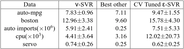
We state the equivalent representer theorem for the choice of kernels and present a semidefinite programming formulation of the resulting optimization problem. Several recipes for constructing hyperkernels are provided, as well as the details of common machine learning problems. Experi-mental results for classification, regression and novelty detection on UCI data show the feasibility of our approach.

Keywords: learning the kernel, capacity control, kernel methods, support vector machines, repre-senter theorem, semidefinite programming

1. Introduction

Kernel methods have been highly successful in solving various problems in machine learning. The algorithms work by implicitly mapping the inputs into a feature space, and finding a suitable hy-pothesis in this new space. In the case of the support vector machine (SVM), this solution is the hyperplane which maximizes the margin in the feature space. The feature mapping in question is defined by a kernel function, which allows us to compute dot products in feature space using only objects in the input space. For an introduction to SVMs and kernel methods, the reader is referred to numerous tutorials such as Burges (1998) and books such as Sch¨olkopf and Smola (2002).

Choosing a suitable kernel function, and therefore a feature mapping, is imperative to the suc-cess of this inference prosuc-cess. This paper provides an inference framework for learning the kernel from training data using an approach akin to the regularized quality functional.

(2)

1.1 Motivation

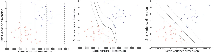
As motivation for the need for methods to learn the kernel, consider Figure 1, which shows the sep-arating hyperplane, the margin and the training data for a synthetic data set. Figure 1(a) shows the classification function for a support vector machine using a Gaussian radial basis function (RBF) kernel. The data has been generated using two Gaussian distributions with standard deviation 1 in one dimension and 1000 in the other. This difference in scale creates problems for the Gaus-sian RBF kernel, since it is unable to find a kernel width suitable for both directions. Hence, the classification function is dominated by the dimension with large variance. Increasing the value of the regularization parameter, C, and hence decreasing the smoothness of the function results in a hyperplane which is more complex, and equally unsatisfactory (Figure 1(b)). The traditional way to handle such data is to normalize each dimension independently.

Instead of normalising the input data, we make the kernel adaptive to allow independent scales for each dimension. This allows the kernel to handle unnormalised data. However, the resulting kernel would be difficult to hand-tune as there may be numerous free variables. In this case, we have a free parameter for each dimension of the input. We ‘learn’ this kernel by defining a quantity analogous to the risk functional, called the quality functional, which measures the ‘badness’ of the kernel function. The classification function for the above mentioned data is shown in Figure 1(c). Observe that it captures the scale of each dimension independently. In general, the solution does not consist of only a single kernel but a linear combination of them.

−3000 −2000 −1000 0 1000 2000 3000 4000 5000 6000 −1 0 1 2 3 4 5

Large variance dimension

Sm a ll v ar ianc e di mens ion

(a) Standard Gaussian RBF kernel (C=10)

−3000 −2000 −1000 0 1000 2000 3000 4000 5000 6000 −1 0 1 2 3 4 5

(b) Standard Gaussian RBF kernel (C=108)

−3000 −2000 −1000 0 1000 2000 3000 4000 5000 6000 −1 0 1 2 3 4 5

(c) RBF-Hyperkernel with adaptive widths

Figure 1: For data with highly non-isotropic variance, choosing one scale for all dimensions leads to unsatisfactory results. Plot of synthetic data, showing the separating hyperplane and the margins given for a uniformly chosen length scale (left and middle) and an automatic width selection (right).

1.2 Related Work

(3)

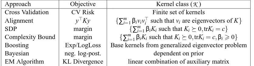
test various simple approximations which bound the leave one out error, or some measure of the capacity of the SVM. The notion of Kernel Target Alignment (Cristianini et al., 2002) uses the ob-jective function tr(Kyy⊤)where y are the training labels, and K is from the class of kernels spanned by the eigenvectors of the kernel matrix of the combined training and test data. The semidefinite programming (SDP) approach (Lanckriet et al., 2004) uses a more general class of kernels, namely a linear combination of positive semidefinite matrices. They minimize the margin of the resulting SVM using a SDP for kernel matrices with constant trace. Similar to this, Bousquet and Herrmann (2002) further restricts the class of kernels to the convex hull of the kernel matrices normalized by their trace. This restriction, along with minimization of the complexity class of the kernel, allows them to perform gradient descent to find the optimum kernel. Using the idea of boosting, Crammer et al. (2002) optimize∑tβtKt, whereβt are the weights used in the boosting algorithm. The class

of base kernels_{Kt}is obtained from the normalized solution of the generalized eigenvector

prob-lem. In principle, one can learn the kernel using Bayesian methods by defining a suitable prior, and learning the hyperparameters by optimizing the marginal likelihood (Williams and Barber, 1998, Williams and Rasmussen, 1996). As an example of this, when other information is available, an auxiliary matrix can be used with the EM algorithm for learning the kernel (Tsuda et al., 2003). Table 1 summarizes these approaches. The notation K0 means that K is positive semidefinite, that is for all a_∈Rn_{, a}⊤_Ka>0.

Approach Objective Kernel class (

K

) Cross Validation CV Risk Finite set of kernels

Alignment y⊤Ky _{∑m_i₌₁βiviv⊤i such that viare eigenvectors of K}

SDP margin _{∑m_i₌₁βiKisuch that Ki0,trKi=c}

Complexity Bound margin _{∑m_i₌₁βiKisuch that Ki0,trKi=c,βi>0}

Boosting Exp/LogLoss Base kernels from generalized eigenvector problem Bayesian neg. log-post. dependent on prior

EM Algorithm KL Divergence linear combination of auxiliary matrix

Table 1: Summary of recent approaches to kernel learning.

1.3 Outline of the Paper

The contribution of this paper is a theoretical framework for learning the kernel. Using this frame-work, we analyze the regularized risk functional. Motivated by the ideas of Cristianini et al. (2003), we show (Section 2) that for most kernel-based learning methods there exists a functional, the

qual-ity functional, which plays a similar role to the empirical risk functional. We introduce a kernel

(4)

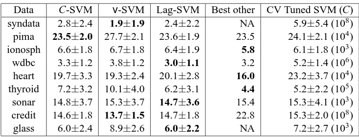
difference in regularization (Ong and Smola, 2003). Details of the specific optimization problems associated with the C-SVM,ν-SVM, Lagrangian SVM,ν-SVR and one class SVM are defined in Section 6. Experimental results for classification, regression and novelty detection (Section 7) are shown. Finally some issues and open problems are discussed (Section 8).

2. Kernel Quality Functionals

We denote by

X

the space of input data and

Y

the space of labels (if we have a supervised learning problem). Denote by Xtrain:={x1, . . . ,xm}the training data and with Ytrain:={y1, . . . ,ym}a set of

corresponding labels, jointly drawn independently and identically from some probability distribu-tion Pr(x,y)on

X

_×

Y

. We shall, by convenient abuse of notation, generally denote Ytrain by the vector y, when writing equations in matrix notation. We denote by K the kernel matrix given by

Ki j:=k(xi,xj)where xi,xj∈Xtrainand k is a positive semidefinite kernel function. We also use trK to mean the trace of the matrix and_|K_|to mean the determinant.

We begin by introducing a new class of functionals Q on data which we will call quality

func-tionals. Note that by quality we actually mean badness or lack of quality, as we would like to

minimize this quantity. Their purpose is to indicate, given a kernel k and the training data, how suitable the kernel is for explaining the training data, or in other words, the quality of the kernel for the estimation problem at hand. Such quality functionals may be the Kernel Target Alignment, the negative log posterior, the minimum of the regularized risk functional, or any luckiness function for kernel methods. We will discuss those functionals after a formal definition of the quality functional itself.

2.1 Empirical and Expected Quality

Definition 1 (Empirical Quality Functional) Given a kernel k, and data X,Y , we define Qemp(k,X,Y)

to be an empirical quality functional if it depends on k only via k(xi,xj) where xi,xj ∈X for

16i,j6m.

By this definition, Qempis a function which tells us how well matched k is to a specific data set X,Y .

Typically such a quantity is used to adapt k in such a manner that Qemp is optimal (for example, optimal Kernel Target Alignment, greatest luckiness, smallest negative log-posterior), based on this one single data set X,Y . Provided a sufficiently rich class of kernels

K

it is in general possible to find a kernel k∗_∈

K

that attains the minimum of any such Qempregardless of the data. However, it is very unlikely that Qemp(k∗,X,Y) would be similarly small for other X,Y , for such a k∗. To measure the overall quality of k we therefore introduce the following definition:

Definition 2 (Expected Quality Functional) Denote by Qemp(k,X,Y) an empirical quality func-tional, then

Q(k):=EX,Y

Qemp(k,X,Y)

is defined to be the expected quality functional. Here the expectation is taken over X,Y , where all xi,yiare drawn from Pr(x,y).

(5)

both cases we compute the value of a functional which depends on some sample X,Y drawn from

Pr(x,y)and a function and in both cases we have

Q(k) =EX,Y

Qemp(k,X,Y)

and R(f) =EX,Y

Remp(f,X,Y)

.

Here R(f) denotes the expected risk. However, while in the case of the empirical risk we can interpret Remp as the empirical estimate of the expected loss R(f) =Ex,y[l(x,y,f(x))], due to the

general form of Qemp, no such analogy is available for quality functionals. Finding a general-purpose bound of the expected error in terms of Q(k)is difficult, since the definition of Q depends heavily on the algorithm under consideration. Nonetheless, it provides a general framework within which such bounds can be derived.

To obtain a generalization error bound, it is sufficient that Qemp is concentrated around its expected value. Furthermore, one would require the deviation of the empirical risk to be upper bounded by Qempand possibly other terms. In other words, we assume a) we have given a concen-tration inequality on quality functionals, such as

Pr

|Qemp(k,X,Y)−Q(k)|>εQ <δQ,

and b) we have a bound on the deviation of the empirical risk in terms of the quality functional

Pr|Remp(f,X,Y)−R(f)|>εR <δ(Qemp). Then we can chain both inequalities together to obtain the following bound

Pr_|Remp(f,X,Y)−R(f)|>εR <δQ+δ(Q+εQ).

This means that the bound now becomes independent of the particular value of the quality func-tional obtained on the data, rather than the expected value of the quality funcfunc-tional. Bounds of this type have been derived for Kernel Target Alignment (Cristianini et al., 2003, Theorem 9) and the Algorithmic Luckiness framework (Herbrich and Williamson, 2002, Theorem 17).

2.2 Examples of Qemp

Before we continue with the derivations of a regularized quality functional and introduce a cor-responding reproducing kernel Hilbert space, we give some examples of quality functionals and present their exact minimizers, whenever possible. This demonstrates that given a rich enough fea-ture space, we can arbitrarily minimize the empirical quality functional Qemp. The difference here from traditional kernel methods is the fact that we allow the kernel to change. This extra degree of freedom allows us to overfit the training data. In many of the examples below, we show that given a feature mapping which can model the labels of the training data precisely, overfitting occurs. That is, if we use the training labels as the kernel matrix, we arbitrarily minimize the quality functional. The reader who is convinced that one can arbitrarily minimize Qemp, by optimizing over a suitably large class of kernels, may skip the following examples.

Example 1 (Regularized Risk Functional) These are commonly used in SVMs and related kernel

methods (see Wahba (1990), Vapnik (1995), Sch¨olkopf and Smola (2002)). They take on the general form

Rreg(f,Xtrain,Ytrain):= 1

m m

∑

i=1

l(xi,yi,f(xi)) +

λ 2kfk

2

(6)

wherekfk2

H is the RKHS norm of f and l is a loss function such that for f(xi) =yi, l(xi,yi,yi) =0.

By virtue of the representer theorem (see Section 3) we know that the minimizer of (1) can be written as a kernel expansion. This leads to the following definition of a quality functional, for a particular loss functional l:

Qregrisk_emp (k,Xtrain,Ytrain):= min

α∈Rm

"

1

m m

∑

i=1

l(xi,yi,[Kα]i) +

λ 2α

⊤_K_α

#

. (2)

The minimizer of (2) is somewhat difficult to find, since we have to carry out a double minimization over K andα. However, we know that Qregriskemp is bounded from below by 0. Hence, it is sufficient if

we can find a (possibly) suboptimal pair(α,k)for which Qregriskemp ≤εfor anyε>0:

• Note that for K=βyy⊤ andα= _βk1_y_k2y we have Kα=y and α⊤Kα=β−1. This leads to l(xi,yi,f(xi)) =0 and therefore Qempregrisk(k,Xtrain,Ytrain) = ₂λ_β. For sufficiently largeβwe can

make Qregriskemp (k,Xtrain,Ytrain)arbitrarily close to 0.

• Even if we disallow setting K arbitrarily close to zero by setting trK=1, finding the minimum

of (2) can be achieved as follows: let K= _k_z1_k2zz⊤, where z∈Rm, andα=z. Then Kα=z and we obtain

1

m m

∑

i=1

l(xi,yi,[Kα]i) +

λ 2α

⊤_K_α₌

∑

m

i=1

l(xi,yi,zi) +

λ 2kzk

2

2. (3)

Choosing each zi=argmin_ζl(xi,yi,ζ(xi))+λ₂ζ2, whereζare the possible hypothesis functions obtained from the training data, yields the minimum with respect to z. Since (3) tends to zero and the regularized risk is lower bounded by zero, we can still arbitrarily minimize Qregriskemp .

This is not surprising since the set of allowable K is huge.

Example 2 (Cross Validation) Cross validation is a widely used method for estimating the

gener-alization error of a particular learning algorithm. Specifically, the leave-one-out cross validation is an almost unbiased estimate of the generalization error (Luntz and Brailovsky, 1969). The quality functional for classification using kernel methods is given by:

Qloo_emp(k,Xtrain,Ytrain):= min

α∈Rm

"

1

m m

∑

i=1

−yisign([Kαi]i)

#

,

which is optimized in Duan et al. (2003), Meyer et al. (2003).

Choosing K=yy⊤andαi=_k_y1i_k2yi, whereαiand yiare the vectorsαand y with the ith element set to zero, we have Kαi=yi. Hence we can match the training data perfectly. For a validation set of larger size, i.e. k-fold cross validation, the same result can be achieved by defining a corresponding α.

Example 3 (Kernel Target Alignment) This quality functional was introduced by Cristianini et al.

(2002) to assess the alignment of a kernel with training labels. It is defined by

Qalignment_emp (k,Xtrain,Ytrain):=1−

tr(Kyy⊤)

ky_k2

2kKkF

(7)

Herekyk2denotes theℓ2 norm of the vector of observations andkKkF is the Frobenius norm, i.e., kK_k2_F :=tr(KK⊤) =∑i,j(Ki j)2. This quality functional was optimized in Lanckriet et al. (2004). By decomposing K into its eigensystem one can see that (4) is minimized, if K=yy⊤, in which case

Qalignment_emp (k∗,Xtrain,Ytrain) =1−

tr(y⊤yy⊤y)

ky_k2₂_kyy⊤_k_F =1−

ky_k4₂

ky_k2₂_ky_k2₂ =0.

We cannot expect that Qalignmentemp (k∗,X,Y) =0 for data other than that chosen to determine k∗, in

other words, a restriction of the class of kernels is required. This was also observed in Cristianini et al. (2003).

The above examples illustrate how existing methods for assessing the quality of a kernel fit within the quality functional framework. We also saw that given a rich enough class of kernels

K

, optimization of Qempover

K

would result in a kernel that would be useless for prediction purposes, in the sense that they can be made to look arbitrarily good in terms of Qempbut with the result that the generalization performance will be poor. This is yet another example of the danger of optimizing too much and overfitting – there is (still) no free lunch.

3. Hyper Reproducing Kernel Hilbert Spaces

We now propose a conceptually simple method to optimize quality functionals over classes of ker-nels by introducing a reproducing kernel Hilbert space on the kernel k itself, so to say, a Hyper-RKHS. We first review the definition of a RKHS (Aronszajn, 1950).

Definition 3 (Reproducing Kernel Hilbert Space) Let

X

be a nonempty set (the index set) and denote by

H

a Hilbert space of functions f :

X

_→R_.

H

is called a reproducing kernel Hilbert space endowed with the dot producth·,_·i(and the normkfk:=p

X

.

2. k spans

H

X

a set, and by l :(

X

_×R2₎m_→R_{∪ {}∞_}_{an arbitrary loss function. Then each}

mini-mizer f _∈

H

of the general regularized risk

(8)

admits a representation of the form

f(x) =

m

∑

i=1

αik(xi,x), (5)

whereαi∈Rfor all 16i6m.

3.1 Regularized Quality Functional

_→R_:

2_{) and the additional condition on k to be symmetric in its first two arguments, and therefore} in its second two arguments as well.

This approach of defining a RKHS on the space of symmetric functions of two variables leads us to a natural regularization method. By analogy with the definition of the regularized risk functional (1), we proceed to define the regularized quality functional.

Definition 6 (Regularized Quality Functional) Let X,Y be the combined training and test set of examples and labels respectively. For a positive semidefinite kernel matrix K on X , the regularized

quality functional is defined as

Qreg(k,X,Y):=Qemp(k,X,Y) + λQ

2 kkk 2

H, (6)

whereλQ>0 is a regularization constant andkkk2_H denotes the RKHS norm in

H

.

(9)

less prone to overfitting than minimizing Qemp, since the regularization term λQ

2 kkk2H effectively

controls the complexity of the class of kernels under consideration. Bousquet and Herrmann (2002) provide a generalization error bound by estimating the Rademacher complexity of the kernel classes in the transduction setting. Regularizers other thankkk2

H are possible, such asℓppenalties. In this

paper, we restrict ourselves to theℓ2 norm (6). The advantage of (6) is that its minimizer satisfies the representer theorem.

Lemma 7 (Representer Theorem for Hyper-RKHS) Let

X

be a set, Qempan arbitrary empirical

quality functional, and X,Y the combined training and test set, then each minimizer k_∈

H

of the regularized quality functional Qreg(k,X,Y)admits a representation of the form

k(x,x′) =

m

∑

i,j

βi jk((xi,xj),(x,x′))for all x,x′∈X, (7)

whereβi j ∈R, for each 16i,j6m.

Proof All we need to do is rewrite (6) so that it satisfies the conditions of Theorem 4. Let x_{i j} := (xi,xj). Then Qemp(k,X,Y)has the properties of a loss function, as it only depends on k via its values at x_{i j}. Note too that the kernel matrix K also only depends on k via its values at x_{i j}. Furthermore,

λQ

2kkk 2

H is an RKHS regularizer, so the representer theorem applies and (7) follows.

Lemma 7 implies that the solution of the regularized quality functional is a linear combination of hyperkernels on the input data. This shows that even though the optimization takes place over an entire Hilbert space of kernels, one can find the optimal solution by choosing among a finite number. Note that the minimizer (7) is not necessarily positive semidefinite. In practice, this is not what we want, since we require a positive semidefinite kernel but we do not have any guarantees for examples in the test set. Therefore we need to impose additional constraints of the type K0 or

k is a Mercer Kernel. While the latter is almost impossible to enforce directly, the former could be

verified directly, hence imposing a constraint only on the values of the kernel matrix k(xi,xj)rather

than on the kernel function k itself. This means that the conditions of the Representer Theorem apply and (7) applies (with suitable constraints on the coefficientsβi j).

Another option is to be somewhat more restrictive and require that all expansion coefficients βi,j >0 and all the functions be positive semidefinite kernels. This latter requirement can be

for-mally stated as follows: For any fixed x_∈

X

the hyperkernel k is a kernel in its second argument; that is for any fixed x_∈

X

, the function k(x,x′):=k(x,(x,x′)), with x,x′_∈

X

, is a positive semidefinite kernel.

Proposition 8 Given a hyperkernel, k with elements such that for any fixed x_∈

X

exp

−λ₂Qkk_k2_H

. (8)

We compare Equation (8) to Gaussian process estimation. The general scheme is known in Bayesian estimation as hyperpriors (Bishop, 1995, Chapter 10), which determine the distribution of the priors (here the GP with covariance k). Figure 2 describes the model of an ordinary GP, where f is drawn from a Gaussian distribution with covariance matrix K and y is conditionally independent given f . For hyperprior estimation, we draw the prior K from a distribution instead of setting it.

Gaussian Process ?>=<89:;? k chosen by user //?>=<89:;K //?>=<89:;f //?>=<89:;y

(11)

To determine the distribution from which we draw the prior, we compute the hyperprior explic-itly. For given data Z=_{X,Y_}and applying Bayes’ Rule, the posterior is given by

p(f_|Z,k) = p(Z|f,k)p(f|k)p(k)

p(k_|Z)p(Z) . (9)

We have the directed graphical model shown in Figure 3 for a Hyperkernel-GP, where we as-sume that the covariance matrix of the Gaussian process K is drawn according to a distribution before performing further steps of dependency calculation. We shall now explicitly compute the terms in the numerator of Equation (9).

Hyperkernel GP ONMLHIJKk0,k p(k|k0,k) /

/?>=<89:;k

p(f_|k)

/

/?>=<89:;f

p(y_|f,x)

/

/?>=<89:;y

Figure 3: Generative model for Gaussian process estimation using hyperpriors on k defined by k.

In the following derivations, we assume that we are dealing with finite dimensional objects, to simplify the calculations of the normalizing constants in the expressions for the distributions. Given that we have additive Gaussian noise, that isε_∼

N

(0,1

γεI), then,

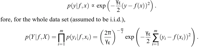
p(y_|f,x)∝exp

−γ₂ε(y₋f(x))2.

Therefore, for the whole data set (assumed to be i.i.d.),

p(Y_|f,X) =

m

∏

i=1

p(yi|f,xi) =

2π γε

−m₂

exp ₋γε 2

m

∑

i=1

(yi−f(xi))2

!

.

We assume a Gaussian prior on the function f , with covariance function k. The positive semidefinite function, k, defines an inner product_h·,_·iHkin the RKHS denoted by

H

k. Then,

p(f_|k) =

2π γf

−F₂

exp₋γf

2hf,fiHk

where F is the dimension of f andγf is a constant.

We assume a Wishart distribution (Lauritzen, 1996, Appendix C), with p degrees of freedom and covariance k0, for the prior distribution of the covariance function k, that is k∼

W

m(p,k0). This is a hyperprior used in the Gaussian process literature:

p(k_|k0) =|

k_|p−(m2+1)exp −1

2tr(kk0)

Γm(p)|k|

p

2

whereΓm(p)denotes the Gamma distribution,Γm(p) =2

pm

2 π

m(m−1) 4 ∏m

i=1Γ

p−i+1 2

. For more de-tails of the Wishart distribution, the reader is referred to Lauritzen (1996).

Observe that tr(kk0)is an inner product between two matrices. We can define a general inner product between two matrices, as the inner product defined in the RKHS denoted by

H

:

p(k_|k0,k) =|k|

p−(m+1)

2 exp −1

2hk,k0iH

Γm(p)|k|

p

2

(12)

We can interpret the above equation as measuring the similarity between the covariance matrix that we obtain from data and the expected covariance matrix (given by the user). This similarity is measured by a dot product defined by k. Substituting the expressions for p(Y_|X,f),p(f_|k)and

p(k|k0,k)into the posterior (Equation 9), we get Equation (10) which is of the same form as the exponentiated negative quality (Equation 8):

exp ₋γε 2

m

∑

i=1

(yi−f(xi))2

!

exp

−γ₂fhf,f_iHk

exp

−1₂hk,k0iH

. (10)

In a nutshell, we assume that the covariance function of the GP k, is distributed according to a Wishart distribution. In other words, we have two nested processes, a Gaussian and a Wishart pro-cess, to model the data generation scheme. Hence we are studying a mixture of Gaussian processes. Note that the maximum likelihood (ML-II) estimator (MacKay, 1994, Williams and Barber, 1998, Williams and Rasmussen, 1996) in Bayesian estimation leads to the same optimization problems as those arising from minimizing the regularized quality functional.

4. Hyperkernels

Having introduced the theoretical basis of the Hyper-RKHS, it is natural to ask whether hyperker-nels, k, exist which satisfy the conditions of Definition 5. We address this question by giving a set of general recipes for building such kernels.

4.1 Power Series Construction

Suppose k is a kernel such that k(x,x′)_≥0 for all x,x′ _∈

X

, and suppose g :R_→R_{is a function}

with positive Taylor expansion coefficients, that is g(ξ) =∑∞_i₌₀ciξifor basis functionsξ, ci>0 for

all i=0, . . . ,∞, and convergence radius R. Then for pointwise positive k(x,x′)_≤√R,

k(x,x′):=g(k(x)k(x′)) =

∞

∑

i=0

ci(k(x)k(x′))i (11)

is a hyperkernel. For k to be a hyperkernel, we need to check that first, k is a kernel, and second, for any fixed pair of elements of the input data, x, the function k(x,(x,x′)) is a kernel, and third that is satisfies the symmetry condition. Here, the symmetry condition follows from the symmetry of k. To see this, observe that for any fixed x, k(x,(x,x′))is a sum of kernel functions, hence it is a kernel itself (since kp(x,x′) is a kernel if k is, for p_∈N_{). To show that k is a kernel, note}

that k(x,x′) =_hΦ(x),Φ(x′)_i, whereΦ(x):= (√c0,√c1k1(x),√c2k2(x), . . .). Note that we require pointwise positivity, so that the coefficients of the sum in Equation (11) are always positive. The Gaussian RBF kernel satisfies this condition, but polynomial kernels of odd degree are not always pointwise positive. In the following example, we use the Gaussian kernel to construct a hyperkernel.

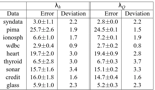
Example 4 (Harmonic Hyperkernel) Suppose k is a kernel with range[0,1], (RBF kernels satisfy this property), and set ci:= (1−λh)λ_hi, i∈N, for some 0<λh<1. Then we have

k(x,x′) = (1₋λh) ∞

∑

i=0

λhk(x)k(x′)

i

= 1−λh

1₋λhk(x)k(x′)

(13)

For k(x,x′) =exp(₋σ2_k_x₋_x′_k2₎_{this construction leads to}

k((x,x′),(x′′,x′′′)) = 1−λh

1₋λhexp(−σ2(kx−x′k2+kx′′−x′′′k2))

. (13)

As one can see, forλh→1, k converges toδx,x′, and thuskkk2_H converges to the Frobenius norm of

k on X_×X .

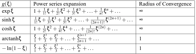
It is straightforward to find other hyperkernels of this sort, simply by consulting tables on power series of functions. Table 2 contains a short list of suitable expansions.

g(ξ) Power series expansion Radius of Convergence expξ 1+_1!1ξ+_2!1ξ2₊ 1

3!ξ3+. . .+ 1

n!ξn+. . . ∞

sinhξ _1!1ξ+ 1 3!ξ3+

1

5!ξ5+. . .+ 1

(2n+1)!ξ(2n+1)+. . . ∞ coshξ 1+ 1

2!ξ 2₊ 1

4!ξ

4₊_{. . .}₊ 1

(2n)!ξ(

2n)₊_{. . .} _∞

arctanhξ ξ₁+ξ₃3+ξ₅5+. . .+ξ_2n2n₊+1₁+. . . 1

−ln(1−ξ) ξ1+

ξ2

2 +

ξ3

3 +. . .+

ξn

n +. . . 1

Table 2: Hyperkernels by Power Series Construction.

However, if we want the kernel to adapt automatically to different widths for each dimension, we need to perform the summation that led to (12) for each dimension in its arguments sepa-rately. Such a hyperkernel corresponds to ideas developed in automatic relevance determination (ARD) (MacKay, 1994, Neal, 1996).

Example 5 (Hyperkernel for ARD) Let kΣ(x,x′) =exp(₋dΣ(x,x′)), where dΣ(x,x′) = (x₋x′)⊤Σ(x₋ x′), andΣis a diagonal covariance matrix. Take sums over each diagonal entryσj=Σj jseparately to obtain

k((x,x′),(x′′,x′′′)) = (1₋λh) d

∑

j=1

∞

∑

i=0

λhkΣ(x,x′)kΣ(x′′,x′′′)

i

=

d

∏

j=1

1₋λh

1₋λhexp

−σj((xj−x′_j)2+ (x′′_j−x′′′_j )2)

. (14)

Eq. (14) holds since k(x)factorizes into its coordinates. A similar definition also allows us to use a distance metric d(x,x′)which is a generalized radial distance as defined by Haussler (1999).

4.2 Hyperkernels Invariant to Translation

Another approach to constructing hyperkernels is via an extension of a result due to Smola et al. (1998) concerning the Fourier transform of translation invariant kernels.

Theorem 9 (Translation Invariant Hyperkernel) Suppose k((x1−x′1),(x2−x′2))is a function which

depends on its arguments only via x1−x′1 and x2−x′2. Let

F

1k(ω,(x2−x′2))denote the Fourier

(14)

The function k is a hyperkernel if k(τ,τ′₎_{is a kernel in}_τ_,_τ′_and

_F

₁_k_(ω_,₍_x′′₋_x′′′₎₎_≥_{0 for all}₍_x′′₋ x′′′)andω.

Proof From (Smola et al., 1998) we know that for k to be a kernel in one of its arguments, its Fourier transform has to be nonnegative. This yields the second condition. Next, we need to show that k is a kernel in its own right. Mercer’s condition requires that for arbitrary f the following is positive:

R

f(x1,x′₁)f(x2,x′₂)k((x1−x′1),(x2−x2′))dx1dx′1dx2dx′2

= R

f(τ1+x′1,x′1)f(τ2+x′2,x′2)dx1,2k(τ1,τ2)dτ1dτ2

= R

g(τ1)g(τ2)k(τ1,τ2)dτ1dτ2,

whereτ1=x1−x′1andτ2=x2−x′2. Here g is obtained by integration over x1and x2 respectively. The latter is exactly Mercer’s condition on k, when viewed as a function of two variables only.

This means that we can check whether a radial basis function (for example Gaussian RBF, exponen-tial RBF, damped harmonic oscillator, generalized Bnspline), can be used to construct a hyperkernel

by checking whether its Fourier transform is positive.

4.3 Explicit Expansion

If we have a finite set of kernels that we want to choose from, we can generate a hyperkernel which is a finite sum of possible kernel functions. This setting is similar to that of Lanckriet et al. (2004).

Suppose ki(x,x′)is a kernel for each i=1, . . . ,n (for example the RBF kernel or the polynomial

kernel), then

k(x,x′):=

n

∑

i=1

ciki(x)ki(x′),ki(x)>0,∀x (15)

is a hyperkernel, as can be seen by an argument similar to that of section 4.1. k is a kernel since

k(x,x′) =_hΦ(x),Φ(x′)_i, whereΦ(x):= (√c1k1(x),√c2k2(x), . . . ,√cnkn(x)).

Example 6 (Polynomial and RBF combination) Let k1(x,x′) = (hx,x′i+b)2p for some choice of

b_∈R+_{and p}_∈N_{, and k}₂₍_x_,_x′_{) =}_exp₍₋σ2_k_x₋_x′_k2₎_{. Then,}

k((x1,x′₁),(x2,x′₂)) =c1(hx1,x′₁i+b)2p(hx2,x′₂i+b)2p

+c2exp(−σ2kx1−x′1k2)exp(−σ2kx2−x′2k2)

(16)

is a hyperkernel.

5. Optimization Problems for Regularized Risk based Quality Functionals

We will now consider the optimization of the quality functionals utilizing hyperkernels. We choose the regularized risk functional as the empirical quality functional; that is we set Qemp(k,X,Y):= Rreg(f,X,Y). It is possible to utilize other quality functionals, such as the Kernel Target Alignment (Example 12). We focus our attention on the regularized risk functional, which is commonly used in SVMs. Furthermore, we will only consider positive semidefinite kernels. For a particular loss function l(xi,yi,f(xi)), we obtain the regularized quality functional.

min

k∈H minf∈Hk

1

m m

∑

i=1

l(xi,yi,f(xi)) +

λ 2kfk

2

Hk+

λQ

2 kkk 2

(15)

By the representer theorem (Theorem 4 and Corollary 7) we can write the regularizers as quadratic terms. Using the soft margin loss, we obtain

min

β minα

1

m m

∑

i=1

max(0,1₋yif(xi)) +

λ 2α

⊤_K_α₊λQ

2 β

⊤_K_β _{subject to} _β_>₀ ₍₁₈₎

whereα_∈Rm_{are the coefficients of the kernel expansion (5), and}β_∈Rm2 _{are the coefficients of}

the hyperkernel expansion (7).

For fixed k, the problem can be formulated as a constrained minimization problem in f , and subsequently expressed in terms of the Lagrange multipliersα. However, this minimum depends on k, and for efficient minimization we would like to compute the derivatives with respect to k. The following lemma tells us how (it is an extension of a result in Chapelle et al. (2002)):

Lemma 10 Let x_∈Rm_{and denote by f}₍_x_,θ)_,_c_i_:Rm_→R_{convex functions, where f is}

parameter-ized byθ. Let R(θ)be the minimum of the following optimization problem (and denote by x(θ)its minimizer):

minimize

x∈Rm f(x,θ)subject to ci(x)≤0 for all 1≤i≤n.

Then∂_θjR(θ) =D₂jf(x(θ),θ), where j_∈N_{and D}₂_{denotes the derivative with respect to the second}

argument of f .

Proof At optimality we have a saddlepoint in the Lagrangian

∂x

L

(x,α) =∂xf(x,θ) + n

∑

i=1

αi∂xci(x) =0. (19)

Furthermore, for allθthe Kuhn-Tucker conditions have to hold, and in particular also∑n_i₌₁αi∂θci(x(θ)) =

0, since for allαi>0 the condition ci(x) =0 and therefore also∂θci(x(θ)) =0 has to be satisfied.

Taking higher order derivatives with respect toθyields

0=∂_θj

"

n

∑

i=1

αi∂xci(x(θ))

∂x ∂θ

#

=∂_θj

−∂xf(x,θ)

∂x ∂θ

. (20)

Here the last equality follows from (19). Next we use

∂j+1

θ f(x,θ) =∂θj

D2f(x,θ) +∂xf(x,θ)

∂x ∂θ

=∂_θjD2f(x,θ). Repeated application then proves the claim.

Instead of directly minimizing Equation (18), we derive the dual formulation. Using the ap-proach in Lanckriet et al. (2004), the corresponding optimization problems can be expressed as a SDP. In general, solving a SDP would be take longer than solving a quadratic program (a traditional SVM is a quadratic program). This reflects the added cost incurred for optimizing over a class of kernels.

(16)

Definition 11 (Semidefinite Program) A semidefinite program (SDP) is a problem of the form: min

x c

⊤_x

subject to F0+

q

∑

i=1

xiFi0 and Ax=b

where x_∈Rp_{are the decision variables, A}_∈Rp×q_{, b}_∈Rp_{, c}_∈Rq_{, and F}_i_∈Rr×r_{are given.}

In general, linear constraints Ax+a>0 can be expressed as a semidefinite constraint diag(Ax+a) 0, and a convex quadratic constraint(Ax+b)⊤₍_Ax₊_b₎₋_c⊤_x₋_d₆_{0 can be written as}

I Ax+b

(Ax+b)⊤ c⊤x+d

0.

When t_∈R_{, we can write the quadratic constraint a}⊤_Aa6t as_kA12ak6t. In practice, linear and

quadratic constraints are simpler and faster to implement in a convex solver.

We derive the corresponding SDP for Equation (17). The following proposition allows us to derive a SDP from a class of general convex programs. It follows the approach in Lanckriet et al. (2004), with some care taken with Schur complements of positive semidefinite matrices (Albert, 1969), and its proof is omitted for brevity.

Proposition 12 (Quadratic Minimax) Let m,n,M_∈N_{, H :}Rn_→_Rm×m_{, c :}_Rn_→_Rm_{, be linear} maps. Let A_∈RM×m_{and a}_∈RM_{. Also, let d :}Rn _→R_{and G}(ξ) _{be a function and the further}

constraints onξ. Then the optimization problem

minimize

ξ∈Rn maximize_x_∈_Rm −

1

2x⊤H(ξ)x−c(ξ)⊤x+d(ξ)

subject to H(ξ)0

Ax+a>0

G(ξ)0

(21)

can be rewritten as

minimize

t,ξ,γ 1

2t+a⊤γ+d(ξ)

subject to



  

diag(γ) 0 0 0

0 G(ξ) 0 0

0 0 H(ξ) (A⊤γ₋c(ξ))

0 0 (A⊤γ₋c(ξ))⊤ t



  

0 (22)

in the sense that theξwhich solves (22) also solves (21).

Specifically, when we have the regularized quality functional, d(ξ)is quadratic, and hence we obtain an optimization problem which has a mix of linear, quadratic and semidefinite constraints.

Corollary 13 Let H,c,A and a be as in Proposition 12, and Σ0. Then the solutionξ∗ to the optimization problem

minimize

ξ maximizex −

1

2x⊤H(ξ)x−c(ξ)⊤x+ 1 2ξ⊤Σξ

subject to H(ξ)0

Ax+a>0 ξ>0

(17)

can be found by solving the semidefinite programming problem

minimize

t,t′_,_ξ_,_γ

1 2t+

1

2t′+a⊤γ

subject to γ>0 ξ>0

kΣ12ξk26t′

H(ξ) (A⊤γ₋c(ξ)) (A⊤γ₋c(ξ))⊤ t

0

(24)

Proof By applying proposition 12, and introducing an auxiliary variable t′which upper bounds the quadratic term ofξ, the claim is proved.

Comparing the objective function in (21) with (18), we observe that H(ξ)and c(ξ)are linear in ξ. Letξ′=εξ. As we varyεthe constraints are still satisfied, but the objective function scales with ε. Sinceξis the coeffient in the hyperkernel expansion, this implies that we have a set of possible kernels which are just scalar multiples of each other. To avoid this, we add an additional constraint onξwhich is 1⊤ξ=c, where c is a constant. This breaks the scaling freedom of the kernel matrix.

As a side-effect, the numerical stability of the SDP problems improves considerably. We chose a linear constraint so that it does not add too much overhead to the optimization problem We make one additional simplification of the optimization problem, which is to replace the upper bound of the squared norm (_kΣ12ξk26t′) with and upper bound on the norm (kΣ

1

2ξk6t′).

In our setting, the regularizer for controlling the complexity of the kernel is taken to be the squared norm of the kernel in the Hyper-RKHS. By looking at the constraints of Equation (24), this is expressed as a bound on the norm (_kΣ12ξk6t′). Comparing this result to the SDP obtained in

Lanckriet et al. (2004, Theorem 16), we see that the corresponding regularizer in their setting is tr(K) =c, where c is a constant. Hence the main difference between the two SDPs is the choice

of the regularizer for the kernel. However, the motivations of the two methods are different. This paper sets out an induction framework for learning the kernel, and for a particular choice of Qemp, namely the regularized risk functional, we obtain an SDP which has similarities to the approach of Lanckriet et al. (2004). On the other hand, they start out with a transduction problem and derive the optimization problem directly. It is unclear at this point which is the better approach.

From the general framework above (Corollary 13, we derive several examples of machine learn-ing problems, specifically binary classification, regression, and slearn-ingle class (also known as novelty detection) problems. The following examples illustrate our method for simultaneously optimizing over the class of kernels induced by the hyperkernel, as well as the hypothesis class of the machine learning problem. We consider machine learning problems based on kernel methods which are de-rived from (17). The derivation is essentially by application of Corollary 13 with the two additional conditions above.

6. Examples of Hyperkernel Optimization Problems

In this section, we define the following notation. For p,q,r_∈Rn_,_n_∈N _{let r}₌_p_◦_{q be defined}

as element by element multiplication, ri =pi×qi (the Hadamard product, or the .∗ operation in

Matlab). The pseudo-inverse (also known as the Moore-Penrose inverse) of a matrix K is denoted

(18)

We define the hyperkernel Gram matrix K by putting together m2 of these vectors, that is we set

K= [~Kpq]m_p_,_q₌₁. Other notations include: the kernel matrix K=reshape(Kβ)(reshaping a m2by 1

vector, Kβ, to a m by m matrix), Y=diag(y)(a matrix with y on the diagonal and zero everywhere else), G(β) =Y KY (the dependence onβis made explicit), I the identity matrix, 1 a vector of ones and 1m_×m a matrix of ones. Let w be the weight vector and boffsetthe bias term in feature space,

that is the hypothesis function in feature space is defined as g(x) =w⊤φ(x) +boffsetwhereφ(·)is the

feature mapping defined by the kernel function k.

The number of training examples is assumed to be m, that is Xtrain=_{x1, . . . ,xm}and Ytrain= y=_{y1, . . . ,ym}. Where appropriate,γandχare Lagrange multipliers, whileηandξare vectors

of Lagrange multipliers from the derivation of the Wolfe dual for the SDP,β are the hyperkernel coefficients, t1and t2are the auxiliary variables. Whenη_∈Rm_{, we define}η>0 to mean that each ηi>0 for i=1, . . . ,m.

We derive the corresponding SDP for the case when Qempis a C-SVM (Example 7). Derivations of the other examples follow the same reasoning, and are omitted.

Example 7 (Linear SVM (C-parameterization)) A commonly used support vector classifier, the

C-SVM (Bennett and Mangasarian, 1992, Cortes and Vapnik, 1995) uses anℓ1soft margin, l(xi,yi,f(xi)) =

max(0,1₋yif(xi)), which allows errors on the training set. The parameter C is given by the user. Setting the quality functional Qemp(k,X,Y) =minf∈H C_m∑mi=1l(xi,yi,f(xi)) +1₂kwk2_H,

min

k∈H minf∈Hk

C m

m

∑

i=1

ζi+

1 2kfk

2

Hk+

λQ

2 kkk 2

H

subject to yif(xi)>1−ζi

ζi>0

(25)

Recall the dual form of the C-SVM,

max

α∈Rm ∑

m

i=1αi−1₂∑mi=1αiαjyiyjk(xi,xj) subject to ∑m_i₌₁αiyi=0

06α_i6C_mfor all i=1, . . . ,m.

By considering the optimization problem dependent on f in (25), we can use the derivation of the dual problem of the standard C-SVM. Observe that we can rewrite _kk_k2_H =β⊤_K_β_{due to the} representer theorem for hyperkernels. Substituting the dual C-SVM problem into (25), we get the following matrix equation,

min

β maxα 1⊤α−

1

2α⊤G(β)α+

λQ

2β⊤Kβ

subject to α⊤y=0 06α6C_m

β>0

(26)

This is of the quadratic form of Corollary 13 where x=α, θ=β, H(θ) = G(β), c(θ) =₋1, Σ=CλQK, the constraints are A=

y ₋y I ₋I ⊤ and a=

(19)

The proof of Proposition 12 uses the Lagrange method. As an illustration of how this proof proceeds, we derive it for this special case of the C-SVM. The Lagrangian associated with (26) is

L(α_,β_,γ_,η_,ξ) =₁⊤α₋1 2α

⊤_G_(β)α₊λQ

2 β

⊤_K_β₊_γ_y⊤_α₊_η⊤_α₋_ξ⊤_(α₋C m1),

whereβ>0,η>0,ξ>0. The minimum is achieved at

α=G(β)†(γy+1+η₋ξ),

and the corresponding dual optimization problem is

minimize

β,γ,η,ξ 1 2z

⊤_G_(β)†_z₊C

mξ

⊤₁₊λQ

2 β

⊤_K_β_,

where z=γy+1+η₋ξ. From this point, we replace the quadratic terms with auxiliary variables t1and t2, and apply the Schur complement lemma (Albert, 1969). The resulting SDP after replacing

kK12βk26t₂bykK

1

2βk6t₂, and introducing the scale breaking constraint 1⊤β=1 is

minimize

β,γ,η,ξ 1 2t1+

C mξ⊤1+

λQ

2t2

subject to η>0,ξ>0,β>0

kK12βk₆t2,1⊤β=1

G(β) z z⊤ t1

0.

(27)

Note that the value of the support vector coefficients, α, which optimizes the corresponding La-grange function is G(β)†z, and the classification function, f =sign(K(α_◦y)₋boffset), is given by

f =sign(KG(β)†₍_y_◦_z₎₋γ)_.

Example 8 (Linear SVM (ν-parameterization)) An alternative parameterization of the ℓ1 soft margin was introduced by Sch¨olkopf et al. (2000), where the user defined parameterν_∈[0,1] con-trols the fraction of margin errors and support vectors. Usingν-SVM as Qemp, that is, for a given ν, Qemp(k,X,Y) =minf∈H _m1∑mi=1ζi+₂1kwk2_H −νρsubject to yif(xi)>ρ−ζi andζi>0 for all i=1, . . . ,m, the corresponding SDP is given by

minimize

β,γ,η,ξ,χ 1

2t1−χν+ξ⊤ 1

m+ λQ

2t2

subject to χ>0,η>0,ξ>0,β>0

kK12βk₆t₂,1⊤β=1

G(β) z z⊤ t1

0

(28)

where z=γy+χ1+η₋ξ.

(20)

Example 9 (Quadratic SVM or Lagrangian SVM) Instead of using anℓ1loss class,

Mangasar-ian and Musicant (2001) use anℓ2loss class,

l(xi,yi,f(xi)) =

0 if yif(xi)>1

(1₋yif(xi))2 otherwise

,

and regularized the weight vector as well as the bias term. The empirical quality functional derived from this is Qemp(k,X,Y) =minf∈H _m1∑mi=1ζ2i +12(kwk

2

H +b2offset)subject to yif(xi)>1−ζi and

ζi>0 for all i=1, . . . ,m. The resulting dual SVM problem has fewer constraints, as is evidenced by the smaller number of Lagrange multipliers needed in the corresponding SDP below.

minimize

β,η 1 2t1+

λQ

2t2

subject to η>0,β>0

kK12βk6t₂,1⊤β=1

H(β) (η+1) (η+1)⊤ t1

0

(29)

where H(β) =Y(K+1m×m+λmI)Y , and z=γ1+η−ξ.

The value ofαwhich optimizes the corresponding Lagrange function is H(β)†(η+1), and the classification function, f =sign(K(α_◦y)₋boffset), is given by f =sign(KH(β)†((η+1)◦y) + y⊤(H(β)†(η+1))).

Example 10 (Single class SVM or Novelty Detection) For unsupervised learning, the single class

SVM computes a function which captures regions in input space where the probability density is in some sense large (Sch¨olkopf et al., 2001). A suitable quality functional Qemp(k,X,Y) = min_f_∈H _νm1 ∑mi=1ζi+1₂kwk2_H −ρsubject to f(xi)>ρ−ζi, andζi>0 for all i=1, . . . ,m, andρ>0. The corresponding SDP for this problem is

minimize

β,γ,η,ξ 1 2t1+ξ⊤

1

νm−γ+λ2Qνt2

subject to η>0,ξ>0,β>0

kK12βk6t₂

K z

z⊤ t1

0

(30)

where z=γ1+η₋ξ, andν∈[0,1]is a user selected parameter controlling the proportion of the data to be classified as novel.

The score to be used for novelty detection is given by f =Kα₋boffset, which reduces to f =

η−ξ, by substitutingα=K†(γ1+η₋ξ), boffset=γ1 and K=reshape(Kβ).

Example 11 (ν-Regression) We derive the SDP for νregression (Sch¨olkopf et al., 2000), which automatically selects the ε insensitive tube for regression. As in the ν-SVM case in Example 8, the user defined parameter ν controls the fraction of errors and support vectors. Using the ε -insensitive loss, l(xi,yi,f(xi)) =max(0,|yi−f(xi)|−ε), and theν-parameterized quality functional, Qemp(k,X,Y) =minf∈H C νε+_m1∑mi=1(ζi+ζ∗i)