www.nonlin-processes-geophys.net/17/65/2010/ © Author(s) 2010. This work is distributed under the Creative Commons Attribution 3.0 License.
Nonlinear Processes
in Geophysics
Inversion of 2-D DC resistivity data using rapid optimization and
minimal complexity neural network
U. K. Singh1, R. K. Tiwari2, and S. B. Singh2
1Department of Applied Geophysics, Indian School of Mines, Dhanbad-826 004, India 2National Geophysical Research Institute, Hyderabad-500 007, India
Received: 7 August 2009 – Revised: 16 November 2009 – Accepted: 2 January 2010 – Published: 3 February 2010
Abstract. The backpropagation (BP) artificial neural
net-work (ANN) technique of optimization based on steepest de-scent algorithm is known to be inept for its poor performance and does not ensure global convergence. Nonlinear and com-plex DC resistivity data require efficient ANN model and more intensive optimization procedures for better results and interpretations. Improvements in the computational ANN modeling process are described with the goals of enhancing the optimization process and reducing ANN model complex-ity. Well-established optimization methods, such as Radial basis algorithm (RBA) and Levenberg-Marquardt algorithms (LMA) have frequently been used to deal with complexity and nonlinearity in such complex geophysical records. We examined here the efficiency of trained LMA and RB net-works by using 2-D synthetic resistivity data and then finally applied to the actual field vertical electrical resistivity sound-ing (VES) data collected from the Puga Valley, Jammu and Kashmir, India. The resulting ANN reconstruction resistiv-ity results are compared with the result of existing inversion approaches, which are in good agreement. The depths and re-sistivity structures obtained by the ANN methods also corre-late well with the known drilling results and geologic bound-aries. The application of the above ANN algorithms proves to be robust and could be used for fast estimation of resistive structures for other complex earth model also.
1 Introduction
Geoelectrical resistivity surveys have been found very useful to map the resistivity structure of complex subsurface geol-ogy (Griffiths and Barker, 1993). The data obtained from
Correspondence to: U. K. Singh
(upendra [email protected])
During the last decade, researches have demonstrated po-tential use of artificial neural networks (ANN) for nonlin-ear inversion and pattern recognition of geophysical data (Raiche, 1991; Poulton et al., 1992; El-Qady and Ushijima, 2001; Singh et al., 2002, 2005, 2006; Zhang and Zhou, 2002; Rummelhart et al., 1986; Roth and Tarantola, 1994). The petroleum industries have also vigorously applied the ANN schemes to process seismic and potential field data (McCor-mack et al., 1993; Brown et al., 1996) to estimate a model that is consistent with the measured data.
However, several problems have been encountered in the use of neural networks. These arise from either designing them incorrectly or by using improper training techniques. The inappropriateness of backpropagation algorithm, for in-stance, for ANN training has been the subject of consider-able research activities. An improvement in the optimization process is therefore essential which will not only speedup the computational process but will also ensure global con-vergence and thereby enhance the quality of result. In this paper, we compared four algorithms using backpropagation neural network, which include the backpropagation algo-rithm (BPA), adaptive backpropagation algoalgo-rithm (ABPA) and Levenberg-Marquardt algorithm (LMA) and algorithm of Radial basis (RBA) network for solving 2-D VES inverse problems. While dealing with synthetic and actual field data, we found that both LMA and RBA based training approaches are efficient in resolving resistivity structure and also com-paratively faster than the other existing methods.
2 Geological setting of the study area
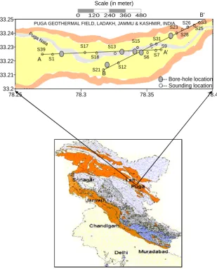
A very brief account of these aspects will be presented be-low. Figure 1a shows the geological and tectonic map of the study area. The Puga Valley is located at an elevation of 4400 m a.m.s.l. in the Ladakh, Jammu & Kashmir, India. In the western and southern part of the Puga Valley, the rock sequence consists of granites and gneisses of unknown age at the base, followed by the Puga formation of probable Pa-leozoic age (Raina et al., 1963). This formation is made up of a lower unit of paragneisses and an upper unit of quartz schist and quartz-mica schist, which at places are gypsifer-ous. Both the quartz and quartz-mica schist contains sul-fur as fillings along the fissures and cracks. The Puga for-mation is seen on both flanks of the Valley and thrust over by a Cretaceous volcanic formation of basic volcanic flows, traps and phyllites in the east. Basic rocks and amphibole-chlorite schist also intrude the Puga formation as dykes and sills. The Valley floor is covered by recent and sub recent deposit of glacial moraines, alluvium; sands spring deposits, sulfur, borax and other hot spring deposits. This loose Valley fills material continuous up to the depths ranging from 15 m to 65 m. Thereafter, hard reconsolidated breccias continues up to the depth of the basement rock i.e. paragneisses and schists (Puga formation). The basement rock intruded by the
Polokongkala granite in the west while, in the east the Samdo formations are exposed. These are comprised of volcanic flow ash beds and associated sedimentary rocks intruded by an ophiolite suite. Along the base of the northern hills in the central part of the Valley sulfur condensates, which are ought to represent an old line of fumarolic activity along a hidden fault (Ravishanker et al., 1976), are found. It should be pointed out, that a prominent N60◦W to S60◦E trending reverse fault. Along the fault, the sequence of paragneiss and schist has been down through towards the southwest with a thin band of impure limestone below the Valley fill material. Several thin limestone bands have been noticed on the north-ern hill scarp of the central part of the Valley. The ultimate heat source for the Puga Valley geothermal field is probably the intrusive rocks lying close to the Valley.
The electrical resistivity depth probes covered the whole area of the Puga Valley, starting from the Samdo confluence on the extreme eastern side to western side, involving a strike length of about 6.5 km. The location of these soundings has been shown in Fig. 1b. On the basis of geological studies, it was thought that the heat derived from magmatic sources travels upward by conduction; the transfer of magmatic heat is greatly facilitated and accelerated by the presence of the deep-seated Zildat fault. This NW-SE trending reverse fault cuts the Puga Valley near the Samdo confluence. In view of the established utility of resistivity method in locating and demarcating potential geothermal areas it was consid-ered worth while to conduct the electrical resistivity depth probe over and near this fault zone in order to get an idea of the resistivity value which could be attributed to the heat source.
3 Theoretical Background
3.1 Artificial Neural Network (ANN)
The ANN processing techniques are based on the analogy of human brain functioning networks. The ANN parallel bio-logical nervous system consists of a large number of simple processing elements with similar number of interconnections among them and is able to collectively solve complicated problems. A three layer schematic nonlinear feed forward neural network(nL,nH,nO)is shown in Fig. 2. The first (in-put) layer consists ofnLnodes, each of which receives one of the input variables. The intermediate (hidden) layer consists ofnH nodes each of which computes a non-linear transfor-mation as described below. The third (output) layer consists
nOnodes, each of which computes a desired output. In ANN processing, a set of inputsα1,α2,α3,...,αnsignals are
mul-tiplied by an associated weightW1,W2,W3,...,Wn before it
is applied to the summation element Net (U).
U=α1W1+α2W2+α3W3+...+αnWn (1)
Fig. 1(a). Geological map of the geothermal area, Puga Valley, Kashmir, India. Fig. 1a. Geological map of the geothermal area, Puga Valley, Kashmir, India.
network is given as follow:
βj(t )=f
Uijh(t )=f nL X
i=0
Wijhαi(t ) !
For j=1,2,3,...,nH (2)
γj(t )=f
Uj ko(t )=f nH X
j=0
Wj koβj(t ) !
For k=1,2,3,...,nO (3)
whereUi∈[−∞ ∞],Ujis bounded on (0 1) for the sigmoid
function, on (-1 1) for the tanh function. Hereαi(t )is the
input to node i of the input layer, and γk(t ) is the output
computed by nodekof the output layer. The input layer bias,
αO=1.0, is included to permit adjustments of the mean level
at each stage. The activation functionsf (.)to be continuous and bounded non-linear logistic sigmoid and hyperbolic tan-gent transfer functions are commonly used:
f1(Uj )= 1
1+e−Uj (4)
f2(Uj )=
1−e−Uj
1+eUj (5)
Fig. 1(b). Tectonically map of the geothermal area, Puga Valley, Kashmir, India.
78.25 78.3 78.35 78.4
33.2 33.21 33.22 33.23 33.24 33.25
A
A'
B
B'
S39
S1
S17
S18
S9
S7 S6 S15 S13
S3 S25 S26
S28 S23
S31
S21 S12
PUGA GEOTHERMAL FIELD, LADAKH, JAMMU & KASHMIR, INDIA.
--- Bore-hole location --- Sounding location Puga N
ala
0 120 240 360 480
Scale (in meter)
Fig. 1b. Tectonically map of the geothermal area, Puga Valley, Kashmir, India.
can be represented as total errorE F (w)=Ep
=1 2
m X
t=1
no
X
k=1
(γPk(t )−OPk(t ))2
Ep
=1 2
m X
t=1
no
X
k=1
f nH X
j=o Wkjo
nl
X
i=0
Wj ihαi(t ) !!
−OPk(t )
!2
WhereENthe error for theN-th input pattern,P is the
num-ber of output, γPk andOPk is the actual and predicted, re-spectively. Here an embedded anomalous was considered to generate a synthetic training datasets that required for train-ing of the network ustrain-ing the finite element forward modeltrain-ing (Uchida, 1991; Dey and Morrison, 1979) scheme as shown in Fig. 3.
3.2 Computational procedure
The computational ANN modeling process may be divided into the following three steps: (i) preprocessing of the In-put data, (ii) determination of the functional form of ANN model, (iii) initialization of the weights, (iv) complexity re-duction through the optimal size of network, and (iv) applica-tion of optimizaapplica-tion algorithm using the appropriate training algorithms.
Fig. 2. Schematic diagram for supervised Artificial Neural Network architecture. 0 0 1 2 3 i 1 2 k 2 1 Input Layer 1.0 1.0 j ) ( ) ( ) ( 3 ) ( 2 ) ( 1 0 . 1 p L n p i p p p α α α α α Hidden Layer Output Layer ) ( 1 p n β ) ( 2 p n β ) ( 3 p n β ) ( ) ( ) ( ) ( ) ( 3 2 1 p p p p p K n J γ γ γ γ γ f ∑ L n H
n nO
) (P j β ) (P h N β In p u t V a ri a b le s O u tp u t V a ri a b le s Bias Units ) ( Resistivity ρ Layer ) (h ness LayerThick Apparent Resistivity Hidden Layer
(Output Layer) (Output Layer) (Input Layer)
Fig. 2. Schematic diagram for supervised Artificial Neural Network architecture.
(ii) Computational neural networks have the ability to ap-proximate any function to any desired degree of accuracy. This universal approximation ability results from the com-bination of sufficient numbers of differently shaped func-tions or neurons in the hidden layers of the ANN. It has been shown that the transfer function must be continuous, bounded and non-constant for an ANN to approximate any function (Hornik, 1991). Such transfer functions include the sigmoid and tanh, the latter is preferred for general purpose use because of its –1 to +1 output range. For the present analysis we used sigmoidal transfer function.
(iii) After deciding the functional form of the ANN model we initialized weight as follows: (a) initialize the hidden layer weights, (b) calculate the sum-squared error (SSE) for that particular ANN model and, and (c) to repeat steps suffi-cient number of times and select the weights with the lowest SSE to provide a good starting point for the optimization pro-cess. The results (Fig. 4) shows that the weight initialization is simple way to determine how many hidden neurons are re-quired to create a satisfactory computational model. Apply-ing the LMA method to same data, but varyApply-ing the number of neurons, gives insight into how many neurons were required.
Fig. 3. The 2-D forward model used to create the resistivity synthetic training and test required for implementing ANN.
-S-4
-S-5 5
5 5 5 5
0 S-3 S-2 S-1 500 m 1000 m D e p th ( m ) 5 Ohm-m 120 Ohm-m
Rectangular Discretization grid 5 Ohm-m 120 Ohm-m
Fig. 3. The 2-D forward model used to create the resistivity syn-thetic training and test required for implementing ANN.
Fig. 4. SSE results of the weight initialization when the number of neurons is varied.
We conducted 10 trials for one to 30 neurons with resulting SSE plotted in Fig. 4. The lower bound of SSE results levels off beginning 18 neurons. The output layer of an over pa-rameterized ANN will be less than full rank because of the multicolinearity of the neurons. A better starting point im-proves the performance of the most optimization algorithms, especially the LMA method.
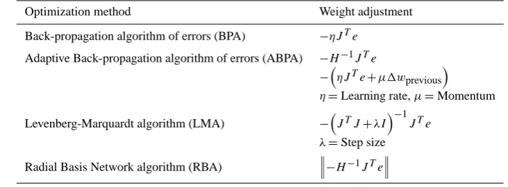
Table 1. A comparison of the initialized weight taken in BPA, ABPA, LMA, and RBA based ANN optimization methods.
Optimization method Weight adjustment
Back-propagation algorithm of errors (BPA) −ηJTe
Adaptive Back-propagation algorithm of errors (ABPA) −H−1JTe −
ηJTe+µ1wprevious
η=Learning rate,µ=Momentum
Levenberg-Marquardt algorithm (LMA) −JTJ+λI
−1
JTe
λ=Step size
Radial Basis Network algorithm (RBA)
−H
−1JTe
the hidden layer should be calculated as follows:
J=m Error
(n+z) (6)
where J= number of neurons in the hidden layer,
m= number of data points in the training set, n = number of inputs andz= number of outputs. Actually no rules exist for determining the exact number of neurons in a hidden layer. In our resistivity inversion, we have taken 18 neurons.
In order to avoid the problem of over-fitting, we performed cross validation with separate set of data solution. Further there is a large amount of redundant information contained in the weights of fully connected network. We found it rea-sonable to prune some weights from the network and at the same time retain the functional capability needed to solve the problem. This has reduced the complexity of the network and made the learning process easier. Secondly at the same num-ber of training samples the reduction of weights leads to the improvement of the generalization ability of neural networks (Haykin, 1994).
The number of hidden layers and neurons is subject to ad-justment in an experimental way by training different struc-tures and choosing one of the smallest one, still satisfying the learning conditions. In our inversion, we have taken the input from Fig. 2 of the ANN architecture with 18 hidden neurons. The network was trained on 75% of the total avail-able data and then tested on 25%. Using LMA, the pruning method with modification was applied on the synthetic re-sistivity data. The results of testing the network before and after regularization are presented in Table 1. This presents the SSE for unpruned and pruned ANN model created for the VES data sets as well as the number of weights in each model before and after pruning. The application of the pruning pro-cedure has resulted in elimination of 179 weights out of 1179 which means more than 15.18% reduction of the number of weights. Testing the original and reduced network on the same data has revealed the overall improvement of predic-tion accuracy on the data.
(v) The mathematical formulas for some of the derivative optimization method generally used in neural networks are shown below in table. Table 1 permits the comparison of the various methods in terms of first and second partial deriva-tives of the error vector ‘e’ with respect to weights in the ANN. Equations (7) and (8) show the formulae for the Jaco-bian (J) and Hessian (H) matrices, the first and second par-tial derivative matrices, respectively (Masters, 1995; Battiti, 1992):
J= ∂e
∂wi
=2e∂y ∂wi
for weight i, desired output y and error e (7)
H= ∂
2e
∂wi∂wj
=2 ∂y
∂wi
· ∂y
∂wj
+e ∂
2y
∂wi∂wj !
for weights i and j (8)
Better approximations to a full Newton’s method optimiza-tion are given by the Levenberg-Marquardt (Levenberg, 1994; Marquardt, 1963) algorithms. Not surprisingly, the LMA method has been shown to outperform both BPA and ABPA in ANN modeling, converging much more rapidly (Hagan and Menhaj, 1994). The LMA approaches the opti-mization process by attempting to utilize some second order information and assumes the second partial derivative com-ponents of the Hessian matrix are insignificant and approx-imates the Hessian with the first term in the Taylor series expansion, JTJ, adjusted by some multipleλof the identity
matrix.
0.001 0.1 10 1000
0 1 2 3 4 5 6 7
Fig. 5. Graphs showing SSE versus time for these paradigms (a) ABP (b) ABPA (c) LMA (d) and RBA
0.001 0.1 10 1000
0 0.2 0.4 0.6 0.8 1 1.2
0.01 0.1 1 10 100 1000
0.01 0.11 0.21 0.31 0.41
0.01 0.1 1
0 0.1 0.2 0.3 0.4
S u m -S q u a re d E rr o r (S S E ) S u m -S q u a re d E rr o r (S S E ) S u m -S q u a re d E rr o r (S S E )
Time (in second)
(a) BPA
(b) ABPA
(c) LMA
(d) RBA
Fig. 5. Graphs showing SSE vs. time for these paradigms (a) ABP, (b) ABPA, (c) LMA, and (d) RBA.
predict the resistivity structure with fraction time. The test data SSE ranged from 0.0130 to 0.0148, equivalent to a 1– 2% error.
4 Application of optimization method
4.1 Synthetic examples
4.1.1 Creation of the 2-D synthetic resistivity structure
We considered an embedded anomalous body of resistivity 120m (Fig. 3) to generate a synthetic training set required for training the network. A collinear Schlumberger was de-ployed in a sounding mode with half of the current electrode spacing 3000 m. The position of the anomalous body was changed and moved to all the model mesh elements. In this approach, we allowed each element in the mesh to be either resistive or conductive. The 2-D data set was generated using the finite element forward modeling (Uchida, 1991; Dey and Morrison, 1979) scheme in which sixty training sets and ten test sets were generated for each profile.
0.01 1 100 10000
0 20 40 60 80 100
Epoch S u m -S q u a re d E rr o r (S S E ) S u m -S q u a re d E rr o r (S S E ) 0.001 0.1 10 1000
0 1 2 3 4 5 6 7 8
-0.1 0.1 0.3 0.5
0 1 2
0.001 0.1 10 1000
0 100 200 300 400 500 600
(a) ABP
(b) ABPA
(c) LMA
(d) RBA
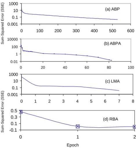
Fig. 6. Graphs showing SSE versus epoch for these paradigms (a) ABP (b) ABPA (c) LMA and (d) RBA.Fig. 6. Graphs showing SSE vs. epoch for these paradigms (a)
ABP, (b) ABPA, (c) LMA, and (d) RBA.
4.1.2 Training and testing of synthetic 2-D resistivity
data
The network was trained by trial and error for each data rep-resentation to produce the lowest errors Training consists of comparison of correct and calculated output patterns and of the adjusting the weights by small amounts1Wij calculated
from the gradient descent rule:
1Wij= −η ∂Ep
∂Wij
(9) This constant term (also called learning rate) governs the rate at the weights are allowed to change at any given presenta-tion. Once the network attains convergence, the weights are adapted and stored in the weight file. Using these updated weights, the network performs the inversion of the field data in few seconds without any more training.
Table 2. Sum squared error (SSE) and number of weights in each model for the unpruned and prned computational ANNN models for the VES data sets.
Sounding Data Set Data SSE for Unpruned Model SSE for Pruned Model
Synthetic Resistivity VES Data Training 0.0125 0.01.40
Validation 0.0130 0.0135
Test 0.0135 0.0.130
Number of Weights 1179 100
Field VLS Data (Case Study-1) Validation 0.0136 0.0140
Test 0.0141 0.0140
Number of Weights 1179 100
Field VLS Data (Case Study-1) Validation 0.0125 0.0155
Test 0.0128 0.0132
Number of Weights 1179 100
Table 3. A comparison of the number if iterations and time taken by the BPA, ABPA, LMA, and RBA methods to converge for synthetic resistivity data sets.
Paradigms Technique Time (in s) Epoch for Convergence Given Epochs Flops
BPA Backpropagation 6.0 529 2000 8 144 355
ABPA Adaptive Backpropagation 1.2 52 2000 1 272 175
LMA Levenberg-Marquardt 0.4 7 2000 809 615
RBA Radial Basis Network 0.3 2 2000 272 772
of different ANN techniques using 2-D resistivity synthetic data. The behavior of the sum-squared network error depicts that the LMA paradigm provides a more stable solution to ar-rive at global minima. With LMA, assign error goal is 0.02, network converges at 7 epochs and the sum square error is 0.0125, which is less than the error goal 0.02. The error be-gins high and decreases as the iteration proceeds until it at-tains an almost constant value of about 0.0125 after 7 epochs, hence the network attains convergence as shown in Table 2. Although the error range lies 0.1–0.2, it is considered very low compared with the other conventional inversion tech-niques i.e. radial error of≤5% (Zohdy, 1989).
4.1.3 Effect of Gaussian noise on model
The apparent resistivity values for Schlumberger multi-electrode system with 28 multi-electrodes are calculated with finite difference program. All possible apparent resistivity values are used as the input data sets. Gaussian random noise of 5% is added to the apparent resistivity values. The resulting apparent resistivity pseudo-section and resistivity section are shown in Fig. 7a, b, and c, respectively. Examples to illus-trate modeling and inversion for each type of 2-D structure are presented here. The starting homogeneous earth model gives an apparent resistivity with RMS error 65%. The RMS
error decreases after each iteration with the largest reduc-tions in the first two iterareduc-tions. The improved LMA con-verges at the 7 iterations with the RMS 0.11 after which no significant improvements were obtained. The inversion were performed both noise free data (Fig. 7c) and data containing 5% (Fig. 7b). Only the results for the noisy data will be pre-sented as they lead to the same conclusions as the noise free data. Plots of the data RMS misfit and of the model RMS misfit versus iteration number are also given for the various model parameters, which can affect the results.
4.1.4 Error calculations
2-D Resistivity model
Fig. 7. Pseudo-section of synthetic resistivity data by (a) conventional method (c) LMA method and Resistivity-section of synthetic resistivity data by (b) conventional method (d) LMA method
Synthetic pseudosection data containing 5% Gaussian noise
2-D resistivity inverted by LMA-ANN model 2 Ωm
4 Ωm
25 Ωm
20 Ωm 30 Ωm
4 Ωm 2 Ωm
120 Ωm
30 Ωm (a)
(b)
(c)
25 Ωm
Error SSE=0.0125 or rms=0.11
Fig. 7. Example to illustrate 2-D inversion of resistivity structure (a) 2-D model, (b) synthetic pseudo-section data containing 5% Gaus-sian noise, and (c) inverted model by LMA method.
From Fig. 5, the BPA, ABPA, LMA and RBA methods took 6, 1.2, 0.4, and 0.3 s to reduce the SSE to 0.01999, 0.0188, 0.0125, and 0, respectively. Besides comparing the time taken by the different inversion methods, it also impor-tant to consider the accuracy of the models obtained. To achieve this, we select the models produced by last two meth-ods, which gives best result within little iterations. The same set of learning parameter values (learning rate, momentum, hidden layer and hidden layer neurons) are used for the all ANN methods. Note that from the second iteration onwards, the SSE achieved by the RBA network is significantly lower than that obtained with the LMA. While the LMA method converges at 7 iterations, which is slower than RBA network. For the RBA method, the SSE is almost zero after 2 iterations as it approaches a minimum point of the objective function. However, for the LMA method, SSE oscillates about the zero and reaches the zero value very fast. Figures 5 and 6 also show that the RBA converges more rapidly than the LMA from the first iteration onwards.
The initial and minimum learning rate and momentum were set 0.001 and 0.8, respectively. Rather small learning parameter can be used. It has been found that small learn-ing rate will slow the convergence but will help to ensure the global minima will not be missed. Large learning rate leads to unstable learning. In order to find an appropriate learning rate and examine its influence the performance of the clas-sifier, the model of the highest resistivity value near sound-ing (S-2) and lowest resistivity value near soundsound-ing (S-5) as shown in Fig. 8. This is the partly a result of equivalence (Keller and Frischknecht, 1996), where a thicker body with low resistivity contrast can give rise to the same anomaly as a thinner block with a higher resistivity contrast.
Fig. 8. Example to illustrate 2-D inversion of resistivity structure (a) 2-D model (b) Synthetic pseudo-section data containing 5% Gaussian noise (c) inverted model by LMA method
2-D resistivity structure by conventional method
2-D resistivity structure by LMA-ANN method (a)
(b)
(c)
(d)
Fig. 8. Pseudo-section of synthetic resistivity data by (a) conven-tional method, (c) LMA method and Resistivity-section of synthetic resistivity data by (b) conventional method, an d(d) LMA method.
Figure 9b (right panel) shows the error contour graph for the optimum solution of the network at the left corner of the error contour map. Figure 9a (left panel) show the 3-D view of the surface error that has a global minimum at center of the plot and local minimum on top of the Valleys produced by synthetic resistivity data. Both plots depict the same scene in different ways. It also shows SSE as a function of epochs for the training of different ANN paradigms. The error be-gins high and decreases as the iteration proceeds until it con-vergences to attain an almost constant value of about 0.0125 after 7 epochs using LMA method (Table 2).
4.2 2-D resistivity field data
4.2.1 Case study-1
Fig. 9. 3-D view of the global and local minima of the ANN net-work using synthetic resistivity data.
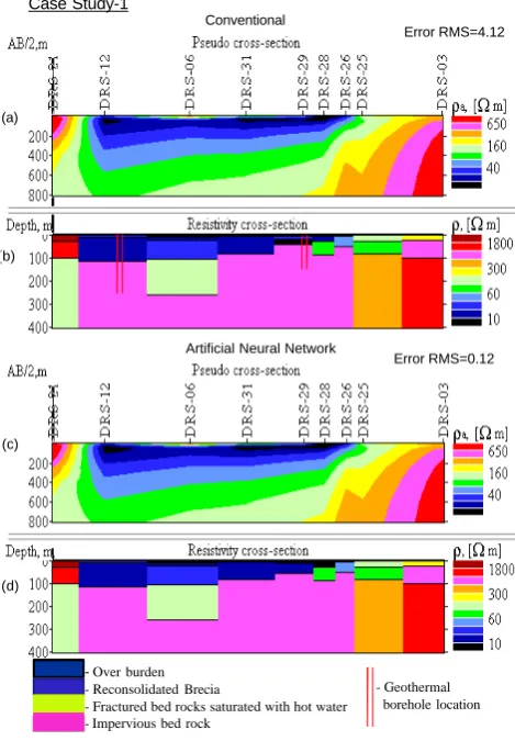
Fig. 10. Pseudo-section of VES field data by (a) conventional method (c) LMA method and resistivity-section of VES field data by (b) conventional method (d) LMA method.
Case Study-1
Artificial Neural Network Conventional
(a)
(b)
(d) (c)
Error RMS=0.12 Error RMS=4.12
-Over burden - Reconsolidated Brecia
- Fractured bed rocks saturated with hot water - Impervious bed rock
- Geothermal borehole location
Fig. 10. Pseudo-section of VES field data by (a) conventional method, (c) LMA method, and resistivity-section of VES field data by (b) conventional method, (d) LMA method.
Fig. 11. Pseudo-section of VES field data by (a) conventional method (c) LMA method and resistivity-section of VES field data by (b) conventional method (d) LMA method
Case Study -2 Conventional
Artificial Neural Network
(c)
(d) (a)
(b)
Error RMS = 2.23
Error RMS = 0.115
-Over burden - Reconsolidated Brecia
- Fractured bed rocks saturated with hot water - Impervious bed rock
- Geothermal borehole location
Fig. 11. Pseudo-section of VES field data by (a) conventional method, (c) LMA method, and resistivity-section of VES field data by (b) conventional method, (d) LMA method.
resistivity value of 277m has been interpreted for the zone between 1.4 m and 21 m of depth below which resistivity val-ues of 700 and 1120m are indicated (Fig. 10). This indi-cates that the resistivity values in this zone are generally more than 100m. While some of established geothermal areas in the world have given resistivity values as low as 5m for the reservoir of geothermal fluids.
4.2.2 Case study-2
The second profile is taken in the E-W direction of the Puga Valley (thermal area), running parallel to the Puga fault and Puga Nala (Fig. 3a). The apparent resistivity pseudo-section (Fig. 11a) and resistivity section (Fig. 11b) show the absence of any conductive zone on the extreme western side after which a thick zone of low resistivity is brought out under the sounding location DRS-37. Further to the east, the con-ductive layer is fairly uniform in thickness with a localized zone of very low resistivity (4–8m). The thinning out of the conductive layer is also brought out on the N-E section (DRS-6 and DRS-7). Thus the results of the resistivity depth probes adequately demonstrate that there are no conductive layers present either on the eastern or on the western side of the Puga Valley that could account for the geothermal man-ifestations in the area. It is also brought out that there is an extensive area underlain by low resistivity formation varying in thickness from 25 to 300 m, invariably resting over very resistive substratum in the central part of the Valley. This is due to the fact that a resistive substratum is present under the entire Valley excludes the possibility of a vertical flow of geothermal fluids under the area surveyed. The fact that high positive S.P. values associated with the low magnetic values and the thinning of the low resistivity zones are observed in the southwestern part of the Valley. It is considered that the geothermal fluids are possibly injected into the Valley from this direction.
Sounding DRS-18 corresponds to the zone of categories (1) and in this curve a very low resistivity formation, with a resistivity of 4m is indicated between the depth of 11 and 36 m. Another such zone encompasses sounding DRS-7 (Fig. 11a), these soundings were conducted near the S.P. positive closures and it is heartening to note that the sounding DRS-7 indicated a resistivity value of about 2m between 19 and 25 m of depth. It may also be noted that the sounding is located near one of the N-S trending features delineated geophysically and is in the vicinity of borehole GW-7 (GSI Technical Report 1976) that gave the maximum discharge of stem during the course of earlier drilling.
It is clear that the present analysis has brought out remark-ably improved the image quality of the conductive layers at different depths. Further existence of the two resistive lay-ers and one conductive layer are now clearly evident. Fig-ure 10c and d shows the recovered layers from the inversion of VES and borehole data at the depth of 350 m. After ap-plying LMA, the data misfit level was reduced to the desired
level. The LMA inversion recovered the true amplitudes of all thin conductive layers very well. Resolution of the con-ductive layer is improved. This suggests that the ANN in-version of the VES data measured at surface is potentially beneficial.
Both profiles show that there is a good correlation between the results of conventional and ANN method. It is obvious that the result obtained from ANN analyses depict some ad-ditional structures, which were not clearly visible in the sec-tion obtained from the convensec-tional techniques. These metic-ulous structures may be related to hydrothermal circulation in the study area. It corresponded well with the drilling and geologic investigation results. Consequently, it is safe to as-sume a high level of reliability.
5 Conclusions
The reliabilities of LMA method using neural network have been demonstrated here to 2-D inversion of VES data and compared to conventional method for two examples of case history. The goal of this investigation was to provide subsur-face information about geoelectrical structure of Puga Valley, Jammu & Kashmir, India. In the present inversion scheme, we compared iterative gradient descent method (BPA and ABPA), Gauss-Newton method known as LMA and RBA interpolation method. Results suggest that LMA and RBA paradigms are considerably faster than the other ANN meth-ods.
We have also examined the effectiveness existing meth-ods generally being used in ANN modeling in an attempt to enhance the optimization process and reduce the model com-plexity. This includes the following three steps in the model-ing process: weight initialization, complexity reduction and application of optimization algorithm. The proposed modifi-cation to the RBA and LMA algorithms performed extremely well and converges more rapidly and with considerably less computational cost for these data than the backpropagation (BPA and ABPA).
The above methods were tested on synthetic VES data as well as on field data collected from Puga Valley. Experiments with above model suggest that the RB is the most convenient paradigm for 2-D inversion of VES data sets. The ANN pro-duced resistivity estimate that was in very close agreement with result of existing methods. Comparatively this paradigm approach has been found to be a fast, efficient, more objec-tive and robust for VES data interpretations.
Acknowledgements. The authors are thankful to both of the
Edited by: Q. Cheng
Reviewed by: P. R. P. Singh and another anonymous referee
References
Battiti, R.: First and second order methods for learning between steepest descent and Newton’s methods, Neural Comput., 4, 141–166, 1992.
Baum, E. and Haussler, D.: What size net gives valid generaliza-tion?, Neural Comput., 1, 151–160, 1989.
Brown, M. and Poulton, M.: Locating buried objects for environ-mental site investigations using neural networks, J. Environ. Eng. Geoph., 1, 179–188, 1996.
Constable, S., Parker, R., and Constable, C.: Occam’s inversion: a practical algorithm for generating smooth models from electro-magnetic sounding data, Geophysics, 52, 4919–4930, 1987. Dahlin, T.: 2-D resistivity surveying for environmental and
engi-neering applications, First Break, 14, 275–284, 1996.
Dahlin, T., Bernstone, C., and Loke, M. H.: A 3-D resistivity in-vestigation of a contaminated site at Lernacken, Sweden, Geo-physics, 67, 1692–1700, 2002.
Dey, A. and Morrison, H. F.: Resistivity modeling for arbitrar-ily shaped two-dimensional structures, Geophys. Prospect., 27, 1020–1036, 1979.
Edwards, L.: SA modified pseudosection for resistivity and induced polarization, Geophysics, 42, 1020–1036, 1977.
Ellis, R. G. and Oldenburg, D. W.: Applied geophysical inversion, Geophys. J. Int., 116, 5–11, 1994.
El-Qady, G. and Ushijima, K.: Inversion of DC resistivity data using neural networks, Geophys. Prospect., 49, 417–430, 2001. Griffiths, D. and Barker, R.: Two-dimensional resistivity imaging
and modeling in areas of complex geology, J. Appl. Geophys., 29, 211–226, 1993.
Hagan, M. T. and Menhaj, M.: Training feed forward networks with the Marquardt algorithms, IEEE T. Neural Networ., 5, 4 pp., 1994.
Haykin, S.: Neural networks: A comprehensive foundation, Macmillan Publishing Co., 1994.
Hornik, K.: Approximation capabilities of multilayer feed forward network, Neural Networks, 4, 251–257, 1991.
Keller, G. V. and Frishchknecht, F. C.: Electrical methods in geo-physical prospecting, Pergamon press, 519 pp., 1996.
Levenberg, K.: A Method for the Solution of Certain Non-Linear Problems in Least Squares, Q. Appl. Math., II(2), 164–168, 1994 Loke, M. and Barker, R.: Rapid least squares inversion of apparent resistivity pseudosections using a quasi Newton’s method, Geo-phys. Prospect., 44, 131–152, 1996.
Marquardt, D. W.: An algorithm for least squares estimation of non-linear parameters, J. Soc. Ind. Appl. Math., 11, 431–41, 1963 Masters, T.: Advanced Algorithm for Neural Networks, Wiley, New
York, 1995.
McCormack, M., Zaucha, D., and Dushek, D.: First break refrac-tion picking and seismic data trace editing using neural networks, Geophysics, 58, 67–78, 1993.
Meju, M.: An effective ridge regression procedure for resistivity data inversion, Computer and Geosciences, 18, 99–118, 1992.
Oldenburg, D. W. and Li, Y.: Estimating the depth of investigation in DC resistivity and IP surveys, Geophysics, 64, 403–416, 1999. Padhi, Ravishanker, Arora, R. N., Gyan Prakash, C. L., Thussa, J. L. and Dua, K. J. S.: Geothermal exploration of Puga and Chumatang geothermal fields, Ladakh, India, in: Proc. UN sym-posium, Development use geothermal resources, 2nd edn., San Francisco, Calif., 245–258, 1992.
Pelton, W., Rijo, L., and Swift, C.: Inversion of two-dimensional resistivity and induced polarization data, Geophysics, 43, 788– 803, 1978.
Poulton, M., Sternberg, K., and Glass, C.: Neural network pattern recognition of subsurface EM images, J. Appl. Geophys., 29, 21– 36, 1992.
Raiche, A.: A pattern recognition approach to geophysical inversion using neural networks, Geophys. J. Int., 105, 629–648, 1991. Raina, B. N., Nanda, M., Bhat, M. L., Mehrotra, P., and Dhalli, B.
N.: Report on the investigations of coal, limestone, borax, and sulphur deposits of Ladakh: Geological survey of India, unpub-lished report, 1963.
Roth, G. and Tarantola, A.: Neural networks and inversion of seis-mic data, J. Geophys. Res., 99, 6753–6768, 1994.
Rummelhart, D. E., Hinton, G. E., and Williams, J.: Learning repre-sentations by back-propagating errors, Nature, 323(9), 533–535, 1986.
Singh, S. B.: Application of Geoelectrical and Geothermal meth-ods for the exploration of geothermal resources in India, Banaras Hindu University, Varanasi, India, 1985.
Singh, U. K., Somvanshi, V. K., Tiwari, R. K., and Singh, S. B.: Inversion of DC resistivity data using neural network approach, IGC-2002, 57–64, 2002.
Singh, U. K., Tiwari, R. K., and Singh, S. B.: One-dimensional in-version of geo-electrical resistivity sounding data using Artificial Neural Networks-a case study, Computers and Geosciences, 31, 99–108, 2006.
Singh, U. K., Tiwari, R. K., Singh, S. B., and Rajan, S.: Prediction of electrical resistivity structures using artificial neural networks, J. Geol. Soc. India, 67, 234–242, 2005.
Sasaki, Y.: Two dimensional joint inversion of magneto-telluric and dipole-dipole resistivity data, Geophysics, 54, 254–262, 1989. Smith, N. and Vozoff, K.: Two-dimensional DC resistivity
inver-sion for dipole-dipole data, IEEE T. Geosci. Remote, 22, 21–28, 1984.
Tripp, A., Hohmann, G., and Swift, C.: Two-dimensional resistivity inversion, Geophysics, 49, 1708–1717, 1984.
Uchida, T.: Two-dimensional resistivity inversion for Schlumberger sounding, Geophysical Exploration of Japan, 44, 1–17, 1991. Zhang, Z., Mackie, R. L., and Madden, T. R.: 3-D resistivity
for-ward modeling and inversion using conjugate gradients, Geo-physics, 60, 1313–1325, 1995.
Zhang, Z. and Zhou, Z.: Real time quasi 2-D inversion or array resistivity logging data using neural networks, Geophysics, 67, 517–524, 2002.