https://doi.org/10.5194/amt-11-593-2018 © Author(s) 2018. This work is distributed under the Creative Commons Attribution 4.0 License.
All-sky photogrammetry techniques to georeference a cloud field
Pierre Crispel1,aand Gregory Roberts1,2
1CNRM, Centre National de Recherches Météorologiques UMR 3589, Météo-France/CNRS, Toulouse, France 2Scripps Institution of Oceanography, Center for Atmospheric Sciences and Physical Oceanography,
La Jolla, California, USA
anow at: Météo-France DSM/AERO, Toulouse, France
Correspondence:Pierre Crispel ([email protected]) and Gregory Roberts ([email protected]) Received: 20 June 2017 – Discussion started: 31 August 2017
Revised: 8 December 2017 – Accepted: 13 December 2017 – Published: 31 January 2018
Abstract.In this study, we present a novel method of identi-fying and geolocalizing cloud field elements from a portable all-sky camera stereo network based on the ground and ori-ented towards zenith. The methodology is mainly based on stereophotogrammetry which is a 3-D reconstruction tech-nique based on triangulation from corresponding stereo pix-els in rectified images. In cases where clouds are horizontally separated, identifying individual positions is performed with segmentation techniques based on hue filtering and contour detection algorithms. Macroscopic cloud field characteristics such as cloud layer base heights and velocity fields are also deduced. In addition, the methodology is fitted to the con-text of measurement campaigns which impose simplicity of implementation, auto-calibration, and portability.
Camera internal geometry models are achieved a priori in the laboratory and validated to ensure a certain accuracy in the peripheral parts of the all-sky image. Then, stereopho-togrammetry with dense 3-D reconstruction is applied with cameras spaced 150 m apart for two validation cases. The first validation case is carried out with cumulus clouds hav-ing a cloud base height at 1500 m a.g.l. The second validation case is carried out with two cloud layers: a cumulus frac-tus layer with a base height at 1000 m a.g.l. and an altocu-mulus stratiformis layer with a base height of 2300 m a.g.l. Velocity fields at cloud base are computed by tracking im-age rectangular patterns through successive shots. The height uncertainty is estimated by comparison with a Vaisala CL31 ceilometer located on the site. The uncertainty on the hor-izontal coordinates and on the velocity field are theoreti-cally quantified by using the experimental uncertainties of the cloud base height and camera orientation. In the first cu-mulus case, segmentation of the image is performed to
iden-tify individuals clouds in the cloud field and determine the horizontal positions of the cloud centers.
1 Introduction
Understanding cloud physical mechanisms is essential for understanding climate and meteorological processes. On cli-mate scales, it is recognized that clouds are a major source of incertitude in atmospheric models (IPCC, 2013), whether for the energy balance or water cycle. Yet, many aspects of cloud’s life cycle are still not understood by the scientific community (Stevens and Feingold, 2009), hence the need for measurement tools allowing cloud monitoring, particularly in a Lagrangian sense.
The use of all-sky cameras makes it possible to widen the field of view.
Stereophotogrammetry applications for use in meteorol-ogy have existed since the beginning of analogue pho-tography (Koppe, 1896; Bradbury and Fujita, 1968), and more recently digital cameras have been used (Allmen and Kegelmeyer, 1997). In the recent years, several technological advances have been made in camera lenses, image resolution, network communications, computational power and cost re-duction. Moreover, major computational improvements have been made in computer vision algorithms, especially in multi-vision reconstruction methods (e.g.,OpenCVlibrary – Bradski and Kaehler, 2008). It is now possible to achieve cloud automatic 3-D reconstruction by stereophotogramme-try relatively cheaply.
Recent studies on this topic generally use conventional or wide-angle lenses to calculate macroscopic characteris-tics of a cloud field, such as cloud base heights and cloud layer horizontal velocities. Seiz (2003) uses a pair of wide-angle cameras spaced 800 m apart and pointing to the zenith to calculate the height of the cloud base. The orientation of the cameras is done using the stars. The errors obtained are about 5 % for mid-altitude clouds at 4000 m a.s.l. Hu et al. (2009) use conventional cameras spaced 1.5 km apart and oriented to mountains to study the three-dimensional organi-zation of orographic convection. The orientation of the cam-eras is achieved using elements of the landscape. Öktem et al. (2014) are interested in the height of maritime clouds with cameras spaced about 900 m apart. The cameras are oriented towards the horizon. They obtained an error in cloud base height of 2 % for low-layer clouds and 8 % for cirrocumulus by comparison with lidar measurements. They also calculate a horizontal velocity field that they compare to the data from a radiosonde. In their case, the orientation of the cameras is achieved by using the position of the sun and the horizon line. In all these previous publications, triangulation is based on the matching of corresponding pixels through the stereo images by manual or automatic methods. In Janeiro et al. (2014), the cloud ceiling information for VFRs (visual flight rules) is calculated by matching a zenith-centered sub-part of the initial stereo images. The authors use low-cost consumer cameras that are oriented towards zenith and spaced about 30 m apart. The orientation of the cameras is achieved using the stars. For clouds under 1500 m a.g.l., which are of prime interest for VFR applications, results at zenith point show good agreement with lidar measurements in single cloud layer situations.
The first study using all-sky cameras in stereophotogram-metry for meteorological purposes is performed by Allmen and Kegelmeyer (1997) to calculate the cloud base height, but temporal synchronization constraints did not allow for usable information to be obtained. More recently, in order to forecast intra-hour solar irradiance, Nguyen and Kleissl (2014) use their own high-resolution all-sky cameras, provid-ing very precise equisolid projection. The cameras are spaced
1230 m apart and the authors use the position of the solar disk to determine orientation. Clouds are filtered in the images with saturation value and cloud base height is determined by plane-sweeping across the stereo images. The results are compared to ceilometer with 8 h time series. Residual mean square deviation of 7 % for cloud base height at 5000 m a.s.l. is obtained. Three-dimensional reconstruction is also per-formed and height distribution of triangulated pixels is com-pared to ceilometer time series showing good agreement. Re-cently, Beekmans et al. (2016) performed a dense 3-D re-construction from a pair of fisheye lens HD cameras spaced 300 m apart. The relative orientation of the cameras is esti-mated using the positions of the stars. This estimation is then refined by an algorithm which automatically matches corre-sponding stereo pixels. The method is validated by compar-ison with the data of a ceilometer, a lidar and a cloud radar for a cloud layer of altocumulus stratiformis at about 3000 m. The results show cloud base height relative errors less than 5 %. The method is then applied to enable a 3-D reconstruc-tion of a developing cumulus mediocris.
In this paper, we use all-sky stereophotogrammetry to per-form geolocation of individual elements of a cloud field in order to follow individual clouds in a Lagrangian way, esti-mate their morphological characteristics and their evolution in real time. Furthermore, this allows the use of cloud geolo-cation for cloud airborne measurements. For example, in the case of instrumented unmanned aerial vehicles (UAVs), the GPS coordinates of the target cloud may be communicated in real time to the autopilot. In addition, installation of a cam-era network for a measurement campaign poses additional challenges. Indeed, it may be difficult, time-consuming, or sometimes impossible to use landscape elements, or the po-sition of the stars. Therefore the methodology, developed in Sect. 2, is based on the principles of simplicity of implemen-tation, auto-calibration, and portability.
3-D reconstruction step consists in finding for each pixel of the left stereo image, its correspondent in the right stereo image. Three-dimensional information is then calculated by triangulation, involving previously calculated camera inter-nal geometry and orientation. In this work, a dense 3-D re-construction is performed by using a block-matching method (Szeliski, 2010) on rectified stereo images (undistortion and misalignment corrections). Additionally, the velocity field is estimated by tracking subparts of the initial image through two successive images and combine this information with the cloud height map. In the case where clouds are suf-ficiently separated to be considered as identifiable objects, we implement image segmentation for individual cloud geo-referencing. We use a color filter to extract the cloud con-tours of the image and use a segmentation algorithm in-spired by Suzuki and Abe (1985) to identify cloud objects. Most of the methodology relies on algorithms implemented in open-source software libraries: OcamCalib(Scaramuzza et al., 2006) for camera calibration, and OpenCV (Bradski and Kaehler, 2008) for the other steps. The accuracy depends on the quality of the cameras and the algorithms used, as well as on the distance between the cameras, with the following paradox: the greater the distance between the cameras, the better the accuracy but the more difficult pixel matching is.
In Sect. 3, we present the results comparing cloud base heights to traditional methods as well as georeferencing indi-vidual cloud elements and calculating the velocity field. The method is applied with cameras spaced 150 m apart, for two validation cases. The first validation case is carried out in the context of a moderately convective situation with isolated cu-mulus clouds with a cloud base height at 1500 m a.g.l. The second validation case is carried out in a situation where two cloud layers overlap: a layer of altocumulus stratiformis with a base height of 2300 m a.g.l. and a layer of cumulus frac-tus with a base height at 1000 m a.g.l. The height uncertainty is estimated by comparison with a Vaisala CL31 ceilometer located on the site. The uncertainty on the horizontal coor-dinates is theoretically quantified by using the experimental uncertainties on the height and uncertainties on the orienta-tion of the cameras. In the cumulus case, a segmentaorienta-tion of the image as well as an estimation of the horizontal positions of the cloud centers is carried out. The results are then dis-cussed in Sect. 4.
2 Material and methods 2.1 Material
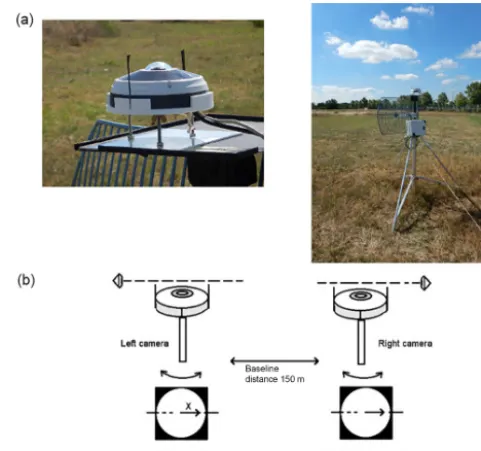
In this work, we use two VIVOTEK FE8391-V network fish-eye cameras designed for outdoor video surveillance appli-cations (see Fig. 1). The focal length is 1.5 mm and the field of view is 180◦. The digital sensor is a 12-megapixel CMOS, providing in its full resolution a 2944 px×2944 px image. The images are transmitted to a computer by a WiFi local
Figure 1. (a)VIVOTEK FE8391-V fisheye camera and installation structure.(b) Vertical sights on the camera housing allow visual inter-camera alignment in the horizontal plane.
network using two directional antennas (TP-Link 2.4 GHz 24 dBi) with several hundred meters of range. Horizontal lev-eling is achieved by the use of a bubble level (accuracy ca. 1◦). The respective positions of both cameras in the Earth frame are evaluated by using GPS, and inter-camera align-ment is achieved with vertical sights on the camera housing. 2.2 Camera projection model, calibration and image
undistortion
Figure 2. Pinhole projection. Physical point M is projected on (u, v)on the image plane(,U,V). Camera coordinate system is defined by axisXandY, which are colinear toU andV, and by axisZ, which is theoptical axis.Principal point(u0, v0)is the pro-jection of theoptical centerOon the image. The radial projected distance on the image is denotedr0.
advantages of this calibration method is its ease of imple-mentation and its accuracy (e.g., Puig et al., 2012, for a com-parative benchmark between several calibration methods for omnidirectional cameras).
2.2.1 Pinhole camera model
The starting point is to consider the simplest camera, that is, the pinholecamera. It is a box that allows the light rays to pass through a small hole pierced on one side. On the op-posite side of the hole, the inverted scene is projected onto a plate. In order to simplify the way in which this projec-tion is represented, a central symmetry is applied to have a situation in which the image plane and the scene are of the same side with respect to the optical center (Fig. 2). The rect-angular image plane has an orthonormal coordinate system (,U,V), whereU is the horizontal axis of the image and
V the vertical axis of the image. The originis located at the upper left corner of the image. The camera reference frame is defined by the orthonormal frame(O,X,Y,Z), whereZ
corresponds to the optical axis directed to the observed scene andXandY correspond to theUandV axes of the image. The point of intersection of the optical axis with the image is calledprincipal point. It does not necessarily coincide with the center of the image, which is especially the case for non-scientific cameras. In this configuration, if (u0, v0)denotes the centered coordinates of a pixel with respect to the prin-cipal point, the projection of a physical point M(x, y, z)is given by the following equation:
u0, v0=(ftan(φ) x/r, ftan(φ) y/r) , (1) wherer=px2+y2denotes the distance from the physical point to the optical axis andφ=arctan(r/z)denotes the an-gle of incidence of the optical ray. The parameter f is the pinhole camera focal length (expressed in pixels in the case of a digital camera). Thus, if(u, v)denotes the pixel
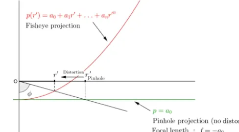
associ-Figure 3. Radial distortion modelization in Scaramuzza et al. (2006) for omnidirectional cameras. Incident angleφand projected radial distancer0are related by tanφ= −r0/p(r0). The polynomial functionpis represented by the red curve. The case where there is no distortion (i.e., pinhole projectionr0=ftanφ) corresponds to a constant polynomial functionp=a0represented by the green line.
ated with theM(x, y, z)point in the frame of the image, the projection is defined by
(u, v,1)T=
1 0 u0 0 1 v0
0 0 1
(u
0, v0,1)T, (2)
where(u0, v0)contains the coordinates of the principal point. We denoteGf,u0,v0
perspective the projection function of parameters {f, u0, v0}which maps a physical pointM(x, y, z)to a pixel (u, v). The reciprocal projection is denoted byG−1f,u0,v0
perspective. It maps an optical ray{λ(x, y,1), λ∈R}to a pixel(u, v). 2.2.2 Omnidirectional Scaramuzza model
Under the axisymmetric assumption, and if r0 denotes the distance between(u, v)and the principal point, Eq. (1) can be generalized to
u0, v0= r0(φ) x/r, r0(φ) y/r. (3) The distance r0 in pixels depends on φ and characterizes the radial distortions. These distortions are preponderant in a fisheye lens. This is the reason why the function r0(φ) is calledrepresentation functionof the fisheye lens. In the Scaramuzza model, this function is implicitly defined by the relation tanφ= −r0/p(r0), wherep(r0)is a polynomial functionp(r0)=a0+a1r0+. . .+anr0n(Fig. 3). The tangen-tial distortions are taken into account linearly by an addi-tional correction step (parametersc,d ande). Thus, if(u, v) denotes the pixel associated with the (x, y, z) point in the frame of the image, the projection is defined by
(u, v,1)T=M(u0, v0,1)T=
1 e u0 d c v0
0 0 1
(u
Figure 4. Calibration procedure by multiple views of the same chessboard. The procedure is automatized by using an algorithmic corner detection. The camera projection function is estimated with the OcamCalibtoolbox following Scaramuzza et al. (2006) mod-elization.
We denoteGM,a0,...,an
fisheye the fisheye projection function of in-trinsic parameters{M, a0, . . ., an}.
2.2.3 Camera calibration method
The camera calibration determines the camera intrinsic pa-rameters {M, a0, . . ., an}. To do this, we use N shots of a chessboard with K1×K2 corners (intersections between black and white tiles – Fig. 4). We denote byRchessboard a coordinate system such that the origin is located on one of these corners, and that the horizontal axes coincide with the chessboard lines. For each shoti, and for each chessboard corner xj, yj,0TR
chessboard, we have the relation (uij, vij)T=GMfisheye,a0,...,an
Ri xj, yj,0
T Rchessboard
+Ti
(5) i=1, . . ., N j=1, . . ., K1×K2,
where(uij, vij)denotes corners positions on the image,Ri the rotation from the camera frame toRchessboardandTi the translation between the optical center of the camera and the origin ofRchessboard. The calibration is based on the follow-ing steps usfollow-ing the toolboxOcamCalib:
1. For each shoti, corners are automatically detected in the image using the intensity gradient specific signal and the pattern of the board (Fig. 4 bottom). This process gives (uij, vij)values.
2. In the nonlinear system (Eq. 5), the values of(uij, vij) and (xj, yj) are known and the system is overdeter-mined for sufficiently large values of N and K1× K2. Parameters {M, a0, . . ., an,{Ri,Ti,∀i=1. . .N}} are determined by using a Marquardt–Levenberg method.
2.2.4 Undistortion
In order to produce undistorted images, the scene is rejected according to a conventional centered perspective pro-jection of focal lengthf. During this reprojection, we move from a circular fisheye image to a square image of size Npx×Npx. The intensity of each pixel of the undistorted im-age is calculated according to the relationship
RGBundistorted(uundistorted, vundistorted)= (6) RGBfisheye
GM,a0,...,an fisheye ·G
−1f,Npx/2,Npx/2 perspective (uundistorted, vundistorted)
.
In this transformation, the peripheral areas are mapped from a given region of the fisheye image onto a larger projection area in the rectified image, producing the blur effect. Note that the values off andNpxcan be freely chosen. The field of view of undistorted images FOVundistorted=2 arctan
Npx 2f will depend on these values. The smaller the value off, the larger the field of view, but the more interpolated areas occupy an important part of the image.
2.3 Orientation, stereo calibration and rectification At the end of the previous step, we are able to produce two undistorted stereo images. They are square images of the same sizeNpx×Npx, for which the center of the image and the principal point coincide, and which would have been taken by two pinhole cameras with the same focal length f. The next step consists in orienting them with respect to each other as accurately as possible. To achieve this, Hu et al. (2009) use landscape features and Öktem et al. (2014) use the horizon line. Seiz (2003) and Beekmans et al. (2016) use the positions of the stars that allows for determining the orienta-tion of each camera. In addiorienta-tion, they add an algorithmic cor-rection step based on SIFT stereo-pixel-matching algorithm (Lowe, 2004). In our work, we develop a visual orientation method assuming that there is no visual obstacle between the two cameras. Like Beekmans et al. (2016), this initial orien-tation is refined by an algorithmic step.
2.3.1 Orientation and stereo calibration
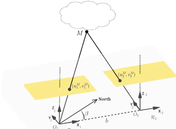
Figure 5.Ideal camera configuration. Camera coordinate systems are frontally aligned with optical axisz1,2oriented towards zenith. Optical centersO1,2are in the same altitude plane. The baseline distance is denotedband North bearing ofO1O2axis is denotedβ. In this ideal configuration, assuming that we have identical pinhole centered cameras, corresponding pixelsuM1 , v1ManduM2 , v2Mare row-aligned on the imagersi.e.,v1M=vM2 .
which needs row alignment of corresponding stereo pixels in the stereo images (see Fig. 5). A refining algorithmic step to calculate the precise relative orientation of the cameras and consequently rectify the stereo images is then required. This procedure is usually referred to asstereo calibrationand consists of calculating the components of the relative rota-tionRand the relative translationT =O1O2between cam-era frames such as(x, y, z)TR1=R(x, y, z)TR2+T.
Stereo calibration is based on the concepts and theorems of epipolar geometry. In particular, in the case of pinhole cam-eras with the same focal lengthf, it exists a constant matrix 3×3 of rank 2 denotedEand calledessential matrix. This matrix only depends onRandT and verifies the following constraint:
u0M2 , v0M2 ,1Eu0M1 , v0M1 ,1T=0, (7)
for all pixels uM1 , vM1 from the left stereo image, and uM2 , vM2 from the right stereo image representing the same physical point M. We use the following stereo calibration methodology:
1. From the undistorted stereo images, retrieve a set of stereo matching pixels with the SIFT algorithm (Lowe, 2004).
2. Using the pairings of step 1, solve the overdetermined system (Eq. 7) whose unknowns are the coefficients of the matrix E. We use a least median of squares (LMEDS) regression, which avoids being affected by outliers. The matrixEis determined to within a scalar factor.
3. Calculate R and T. For this purpose, the following equations are used:
[T×]2= −EET (8)
with[T×] =
0 −Tz Ty
Tz 0 −Tx
−Ty Tx 0
,
which give two opposite solutionsT+andT−and
R= 1
4. Corrective rotationsR1andR2are defined by usingR andT such that
R1=R−rect1 andR2=R−rect1R, (10)
whereRrect=(e1,e2,e3)is a rotation matrix such ase1 is oriented in the same direction ofT, ande2is orthog-onal toe1and to the left camera optical axis.
5. Consistency step: initial visual orientation of the cam-eras is achieved to be as close as possible to the frontally aligned relative orientation (i.e., R'Id and
T '(b,0,0)T; see Sect. 2.3). In our algorithm, several estimations of the essential matrixE, and consequently R and T, are achieved to avoid incorrect solutions which are due to erroneous or imprecise matches in the SIFT procedure. These estimations ofEare obtained by using several subsets of the matching pixel set given by the SIFT procedure. Estimations ofEmatrix, which are not coherent with theR'Id andT '(b,0,0)T hypoth-esis, are then rejected. Among the coherent estimations, we choose the one that leads to minimal corrective rota-tions.
2.3.2 Rectification
We use R1 andR2to produce undistorted rectified images; that is, the images that would have been produced by per-fectly aligned pinhole cameras. These images are produced from all-sky original images by the following transformation: RGBCAM1,2rectified (urectified, vrectified)= (11) RGBCAM1,2fisheye GintrinsicparamsCAM1,2fisheye ·G−perspective1f,Npx/2,Npx/2
·R1,2(urectified, vrectified,1)
.
2.4 Three-dimensional reconstruction
Three-dimensional reconstruction is obtained by triangula-tion from two pixels uM1 , v1M and uM2 , v2M which are known to represent the same physical point M. Indeed, knowing the projection functions of each camera, their rel-ative orientations, and the distance between the cameras, it is possible to estimate the point of intersection of the opti-cal rays in a given reference frame. Working directly with the rectified images make this calculation easier because we have a simple theoretical standard situation: identical pinhole images in a frontally aligned orientation (Fig. 5 right). In this case, two matching pixels are located on the same row in the image matrices i.e., v1M=v2M. Then, the coordinates (xM, yM, hM) in the rectified frame of the left camera are
given by
hM= f b
uM2 −uM1 = f b
δM, (12)
xM=hM u0M1
f , yM=hM v0M1
f ,
whereδM=uM2 −uM1 is calleddisparityand is linearly re-lated tohthrough the baseline distance between the cameras b, and the focal distancef.
In addition, a dense 3-D reconstruction of the observed scene assumes that one is able to generate a dense match-ing of correspondmatch-ing pixels across the stereo images. This is called the dense stereo matching problem. In the case of rectified images, this problem is greatly simplified by the fact thatv1M=v2M and thus becomes a one-dimensional problem. In this case, a very common method is the block-matching algorithm (Szeliski, 2010), which relies on find-ing maximum correlations between neighborhoods of pix-els across the stereo images. This algorithm is implemented in the OpenCV library (Bradski and Kaehler, 2008), and is able to describe finely the variations of altitude. However, it generates noise/speckles in the weakly textured image part, which is a disadvantage for the type of objects that we con-sider (clouds, blue sky background, sun). To avoid this effect, we use several techniques:
– Adjusting algorithm parameters:
– Disparity range is limited during the pixel-matching process by setting minimum and maxi-mum bounds for cloud height detection. Note that disparity bounds are related to height detection bounds with equation (Eq. 12), even if this relation-ship becomes less relevant for larger incident angles for which larger horizontal errors occur.
– Window correlation size is adjusted to prevent speckles.
– Smoothing the signal by reducing the size of the image while taking advantage of the subpixel resolution of the algorithm.
– Using blue sky filtering: we process the altitude map by filtering the blue sky areas. We use image conversion in the HSV (hue, saturation, value) color management system. The hue values ranging from 170 to 280◦(from cyan to violet) are filtered.
2.5 Velocity field
Figure 6.Multiblock tracking algorithm for cloud field velocity es-timation. For each blockIk1,k2, the velocity vector is computed by using the displacement vector1k1,k2 expressed in pixels and the median altitudehk1,k2. Displacement vector is computed by using the Lewis (1995)’s matching template algorithm. Computations are based on two successive rectified images: in our case we use the left rectified image at timest1andt2.
on the image is converted into velocity by using the previ-ously calculated height map. In practice, the initial image is divided into rectangular blocksIt1
k1,k2 indexed by the sub-scriptsk1,2(Fig. 6). The median of heightshk1,k2 is assigned to these blocks based on the cloud height map. The transla-tion in number of pixels of each block through two succes-sive shots is denoted by1k1,k2. It is related to the block mean horizontal velocityvkx
1,k2, v y k1,k2
by
vxk 1,k2 =
hk1,k2 f
1uk 1,k2
1t , (13)
vyk 1,k2 =
hk1,k2 f
1vk 1,k2 1t ,
where1t=t1−t2is the time between two shots. Calculating 1k1,k2 is to determine the position of aI
t1
k1,k2 template in the It2 image. This generic computer vision problem is called template matching. A method developed by Lewis (1995) and based on the normal cross correlation index allows per-forming this search with a low algorithmic cost in simple cases (no rotation, no scaling). This algorithm is available in the OpenCV library (Bradski and Kaehler, 2008).
Note that the technique used here is similar to that used by Janeiro et al. (2014), which evaluates the displacement of a single block centered on the principal point through two images. In our case, the approach is multiblock, which gener-ates dispersion but makes it possible to estimate the velocities of multiple cloud layers.
2.6 Segmentation and cloud identification
Segmentation techniques are used in computer vision prob-lems to identify objects in an image. In our case, the main interest of this technique is to identify and georeference indi-vidual clouds when the situation allows it. The method that
we present here is a contour-based method involving blue sky filtering which supposes that the clouds are separated (e.g., cumulus cloud field) and that they do not overlap on the im-age due to projection (this would result in merged contours). Segmentation is achieved with the following steps:
1. Production of a binarized image from blue sky filter (Sect. 2.4).
2. Contour detection and segmentation using the binarized image: we use a contour finding algorithm implemented in OpenCV library and inspired by Suzuki and Abe (1985).
3. Filtering non-significant/noisy contours: we eliminate contours with a low inside area, and with a low num-ber of inner triangulated pixels.
4. Filtering sun: we use a threshold on altitude to remove the sun.
Each segmented region contains pixels that have been trian-gulated in the 3-D reconstruction process. This allows as-signing(x, y, z) coordinates for each triangulated pixel. In order to avoid outliers the center of each segmented cloud, and the cloud base height is estimated with
xcenter=
q5(x)+q95(x)
2 , ycenter=
q5(y)+q95(y)
2 , (14)
zcloudbase=q10(z)
wherex,y,zcorresponds to coordinates of all triangulated pixels within the segmented region. The notationqr(x)(ory andz) denotes therth quantile ofxvalues (oryandz) within the segmented region.
2.7 Uncertainty estimation
Theoretically, in a frontally aligned pinhole stereo system, the uncertainty on heightσh can be related to the uncertain-ties on the position of corresponding pixels(u1, v),(u2, v), given by the sensitivity equation
σh=σ|u1−u2| h2 f b=σδ
h2
f b. (15)
whereσ|δ|=σ|u1−u2| represents the uncertainty on disparity (Sect. 2.4). This equation shows that uncertainty decreases linearly as the baseline distancebincreases, until a distance where the quality of the stereo-pixel-matching degrades. On the other hand, σh quadratically increases with increasing heights.
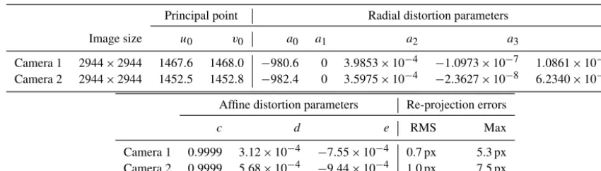
Table 1.OcamCalib calibration results for cameras 1 and 2. Parameters are described in Eqs. (3) and (4) in Sect. 2.2.
Principal point Radial distortion parameters
Image size u0 v0 a0 a1 a2 a3 a4
Camera 1 2944×2944 1467.6 1468.0 −980.6 0 3.9853×10⁻⁴ −1.0973×10⁻⁷ 1.0861×10⁻¹⁰ Camera 2 2944×2944 1452.5 1452.8 −982.4 0 3.5975×10⁻⁴ −2.3627×10⁻⁸ 6.2340×10⁻¹¹
Affine distortion parameters Re-projection errors
c d e RMS Max
Camera 1 0.9999 3.12×10⁻⁴ −7.55×10⁻⁴ 0.7 px 5.3 px Camera 2 0.9999 5.68×10⁻⁴ −9.44×10⁻⁴ 1.0 px 7.5 px
this work, we use a Vaisala CL31 ceilometer, collocated with the all-sky stereo system, as the reference instrument. It pro-vides information by measuring the cloud base height at the zenith and identifies up to three cloud layers. Several aspects must be identified before comparing ceilometer and all-sky stereo system results:
1. There is spatial inter-cloud and intra-cloud variability of the cloud base height.
2. All-sky stereo system computes heights coming from the base as well as the sides of the clouds.
3. Ceilometer provides a point value at zenith, while the cameras provide a spatial map of the heights.
4. All-sky stereo system can recover multiple cloud heights only if it can see them.
Several methodologies can be used to compare all-sky spa-tial data to ceilometer temporal data. A comparison of height measurements at zenith when the picture is taken allows estimating uncertainty on height σh, although this method is limited because it does not represent the uncertainty on the peripheral parts of the image. Another way is to com-pare the height–frequency histograms obtained by the all-sky stereo system (heights calculated for a scene) with the distri-bution of the heights obtained by the ceilometer (centered time series). The distribution peaks represent the represen-tative height of the cloud base for a given cloud layer. The thickness associated with these peaks is due to the above-mentioned uncertainties and cloud base variability. The error is estimated by comparing the peak positions and the stan-dard deviations of the distributions around these peaks.
In the Earth frame, the uncertainty on(x, y)position can be deducted from uncertainties on height σh, polar angle σφ, and azimuthal angleσθ. Indeed, in spherical coordinates we have x=ρcosθsinφ,y=ρsinθsinφ,h=ρcosφ. By denoting r=px2+y2=htanφ, the ground projected dis-tance, we obtainx=hcosθtanφandy=hsinθtanφ, such
that
σx2=(cosθtanφ)2σh2+(hsinθtanφ)2σθ2 (16) +(hcosθcos−2φ)2σφ2,
σy2=(sinθtanφ)2σh2+(hcosθtanφ)2σθ2 (17) +(hsinθcos−2φ)2σφ2,
σr2=tan2φ σh2+h2cos−4φ σφ2. (18) The angle uncertainties are mainly related to the orientation of the cameras: initial orientation (GPS position and visual sighting) and algorithmic correction in the rectification pro-cess (Sect. 2.3). In our study, the estimation of σh is cal-culated experimentally as mentioned above. The corrective rotations provided by the rectification algorithm in differ-ent configurations allows estimating σθ andσφ, providing σθ=σφ=2◦.
3 Results
3.1 Camera calibration
Figure 7. (a)Radial projected distancer0as a function of incident angleφfor VIVOTEK camera 1. Functionr0(φ)is calledrepresentation functionas it characterize the projection. It is compared to the mostly used fisheye parametric representation functions set with−a0value forf.(b)difference in pixels between representation functions of cameras 1 and 2, as a function of incidence angleφ.
Figure 8.For each view and each chessboard corner (which represents an amount of 30×48 points), difference between corner position on the image, and corner position computed by re-projection, usingOcamCalibcalibration results.
of the cameras 1 and 2 is shown in Fig. 7b. The calculation of sensitivity dφ/dr0allows estimating the uncertainty on the angle of incidenceφ. In our case, this uncertainty varies as a function ofφbetween 0.06 and 0.07◦px−1. Finally, Fig. 8 illustrates the dispersion of the reprojection errors for each corner and for each shot.
The result of this calibration shows that both all-sky cam-eras obtain an intermediate projection between the equidis-tant and equisolid projections (Fig. 7a), with the difference increasing significantly beyond an incident angle of 50◦ (10 px deviation/angular error of 0.65◦). This shows that the use of a precise calibration model and method is needed if one wishes to use the peripheral parts of the all-sky image. The difference between the representation functions of the camera 1 and the camera 2 (Fig. 7b) shows that the fisheye projections are almost identical up to an angle of incidence of 70◦(2 px deviation), which is an indicator of validity of the calibration. This uncertainty increases significantly beyond
angles greater than 80◦. The dispersion of the reprojection error is small (Table 1, Fig. 8) with an average reprojection error less than 1 px (i.e., 0.065◦) and 7 px (i.e., 0.5◦) maxi-mum deviation.
3.2 Georeferencing results 3.2.1 Validation cases
Table 2.Description of validation cases.
Validation case 1 Validation case 2
Place Toulouse – Météo France
Date (UTC) 8 July 2016 13:55 16 June 2016 10:00
Shots 3 shots every 15 min
Baseline distance between cameras,b 147 m±3 m
Type of clouds cumulus humilis and cumulus fractus and mediocris altocumulus stratifromis
Mean cloudiness 50 % (4 octas) 75 % (6 octas)
Mean cloud base height 1500 m a.g.l. 1000 and 2300 m a.g.l.
Ceilometer Frequency: 1 min; start/end time of temporal series:
±15 min before and after camera shot
Table 3.Algorithm parameters.
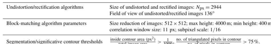
Undistortion/rectification algorithms Size of undistorted and rectified images:Npx=2944 Field of view of undistorted/rectified images 136◦
Block-matching algorithm parameters Size reduction of images: 512×512; max height: 4000 m; min height: 400 m; correlation window size: 11 px; subpixel scale: 1/16
Segmentation/significative contour thresholds inside contour areatotal image area(px2)>10001 ,no.of triangulated pixels in contourno.of pixels in contour >75 %.
validation case occurred around noon, highlighting the de-tection of multiple cloud layers (June 2016). The clouds are cumulus fractus with cloud base at 1000 m a.g.l. and altocu-mulus stratiformis with bases at 2300 m a.g.l. The cloudiness is about 6 octas. In this case, we have a ratioh/b≤15. The context of each test case is summarized in Table 2.
3.2.2 Cloud height map
For each validation case, we repeat the same procedure three times at intervals of 15 min.
1. Capture and undistortion of the fisheye images (Sect. 2.2).
2. Stereo pixel matching and stereo calibration (Sect. 2.3). 3. Rectification of the undistorted images (Sect. 2.3). 4. Three-dimensional reconstruction and calculation of the
height map (Sect. 2.4).
5. Comparison with a ±15 min time series from the ceilometer (Sect. 2.7).
Note that in operational situations, the stereo calibration (step 2) does not need to be performed before each shot if the material stays in place. Since we quantify the error as-sociated with the entire methodology, step 2 is re-executed
for each shot. In step 4, smoothing and filtering techniques to avoid speckles in non-textured zones are implemented (Sect. 2.4). In particular, min/max threshold on heights is set toh∈[450 m, 4000 m] and a blue-sky filter is implemented. The parameters for image undistortion, rectification, 3-D re-construction and segmentation are given in Table 3.
We compare the distributions of the heights obtained with the all-sky stereo system to the ceilometer. The results ob-tained for the first and second case are presented in Figs. 9 and 10, respectively, with images spaced 15 min apart. On those panels, the top row represents the undistorted and rec-tified images of the left camera at each time interval. The middle row represents cloud height maps. The bottom row represents the distributions of the calculated heights (blue histograms) compared with the ceilometer distributions (red histograms). In addition, ceilometer and all-sky system cloud base height estimations at zenith are given for each time. The comparison of ceilometer and all-sky system height distribu-tions is summarized in Fig. 11.
Figure 9.Cumulus validation case – height map and distribution for three shots evenly spaced of 15 min. Panel(a)represents the left camera images. Panel(b)represents the associated height map computed by the stereovision system. Panel(c)represents the frequency histogram of heights computed by the stereovision system (blue diagram – 100 m bins). This distribution is compared to the ceilometer frequency histogram (red curve – 100 m bins).
100 m, which is similar to the ceilometer. As expected, in-stantaneous comparison at zenith gives better accuracy re-sults with a measurement difference up to 50 m (i.e.,σh/ h' 3 %).
The results of the second validation case (altocumulus/multi-layer) show that all-sky camera net-work can identify multiple cloud layers. In this case, the offset between distribution peaks is 20 m for the lower cu-mulus fractus cloud layer (h=1000 m a.g.l.). For the layer at 2300 m a.g.l., the offset on the distribution peak varies between 60 m (second image) and 350 m (three image). In this case, where h/b=15, the ratio σh/ h'15 %. As previously stated, standard deviations obtained by the cam-eras and the ceilometer are similar around the peak values, varying between 100 and 200 m. For this case, instantaneous comparison at zenith gives a measurement difference up to 100 m for the 2300 m layer (i.e.,σh/ h'5 %).
From these experiments, using peak distribution offsets, we note that σh/ h'0.01h/b can be considered as a gen-eral rule for the height measurement uncertainty when using our methodology. The stereo calibration step is most likely responsible for the observed shifts. As we have explained in Sect. 2.3, this step is sensitive to the quality of the pixel matching performed by the SIFT method. This is illustrated by Fig. 12 showing variability of the height distribution with
different stereo calibrations in the altocumulus case. Accord-ing toσh/ hrelationship, sensitivity on the stereo calibration step increases when ratioh/bincreases. Indeed, in this exam-ple, the peak corresponding to the low-layer cumulus fractus clouds ('1000 m) is barely impacted by the stereo calibra-tion step.
3.2.3 Horizontal georeferencing results, velocity map and segmentation
The horizontal georeferencing and velocity results obtained for the cumulus and altocumulus/multi-layer cases are shown in Figs. 13 and 14, respectively. For each figure, we show the left camera rectified image and its associated velocity map (top figures), the 3-D point cloud projection on the left camerax−y horizontal plane, and uncertainty on position σr (bottom figures). This uncertainty is estimated using the Eq. (18) withσφ=2◦, andσh=0.01h2/baccording to the experimental results presented in the previous section.
Figure 10.Altocumulus/multilayer validation case – height map and distribution for three shots evenly spaced of 15 min. Panel(a)represents the left camera images. Panel(b)represents the associated height map computed by the stereovision system. Panel(c)represents the frequency histogram of heights computed by the stereovision system (blue diagram – 100 m bins). This distribution is compared to the ceilometer frequency histogram (red curve – 100 m bins).
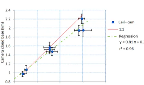
Figure 11.Comparison of mean cloud base height results obtained by the camera stereovision system and mean cloud base height re-sults obtained by the ceilometer (blue points). The red 1 : 1 line cor-responds to the reference plot. Linear regression for the ceilometer-camera plot is shown by the green dashed line.
450 m for a cloud located at 3 km. The estimated velocity is 14 km h−1with a mean direction of wind of 255◦.
For the multi-layer/altocumulus case, the uncertainty is 180 m for a cloud at 1 km, 330 m for a cloud at 2 km and 500 m for a cloud at 3 km. The velocity results show that the all-sky stereo system is able to estimate the velocities of
dif-ferent cloud layers. In this case, the estimated average ve-locity is 16 km h−1 for the 1000 m layer and 30 km h−1 for the 2300 m layer, with respective mean directions of 205 and 230◦.
We note that the uncertainty on cloud layer velocity is re-lated tohfollowing Eq. (13), and is between 10 and 15 % in the cases studied.
In the cumulus mediocris case, as we have separated cumulus clouds on the images, the situation allows go-ing further and implementgo-ing the segmentation algorithm (Sect. 2.6). Results are shown in Fig. 15. We show the cloud height map, as well as the segmented image with the esti-mated positions of cloud centers (red dots and cloud iden-tification number). The estimated cloud positions are listed in Table 4. The estimated individual cloud base heights are compared with the ±15 min ceilometer time series. In our case, we find that the all-sky camera network allows identi-fying clouds as individual objects. The estimated cloud base heights agree well with the ceilometer.
4 Discussion and future work
applica-Figure 12.Sensitivity of the stereo calibration step illustrated by the first shot in the altocumulus validation case. For this shot, we represent the height–frequency histogram obtained with(a)no stereo calibration,(b)stereo calibration parameters obtained with the first shot pair of images, and(c)stereo calibration parameters obtained with the second shot pair of images.
Figure 13.Cumulus case.(a, b)Rectified image(a)with estimated wind speed and direction(b).(c, d)Triangulated points projected on x−yleft camera plane with altitude color map(c), and withr-incertitude color map(d).
tions by instrumented UAVs. Yet, for precise measurements – morphological parameters of a cloud (width, vertical exten-sion and variation over time), and precise geolocation (e.g., measurements near the base, top, or edges of the cloud) – the all-sky camera network must be configured to ensure a certain accuracy.
In addition to optimizing the baseline distance between the cameras, several strategies can be explored to improve the ac-curacy of all-sky camera system. A first strategy is to work on the robustness of the orientation step. Relative orientation accuracy between stereo cameras plays an important role in the image rectification process (Sect. 2.3). Indeed, relative
orientation has an impact on 3-D reconstruction accuracy through pixel-matching hit score, and uncertainty on dispar-ity, as shown with Eqs. (12) and (15), and experimentally in Fig. 12. Moreover, it is important to ensure that cameras are correctly oriented in the Earth’s frame for accurate geolocal-ization, as shown in Eq. (18).
Table 4.Segmentation and geolocalization results.
Cloud ID Estimated cloud base Position(x, y)of cloud centers r σr height (m a.g.l.)±10 % in the left rectified coordinate system
3 1440 (−2.69 km, 1.75 km) 3.21 km ±350 m 5 1670 (2.41 km, 1.55 km) 2.87 km ±290 m 6 1420 (−1.83 km, 1.46 km) 2.34 km ±260 m 7 1450 (−1.80 km,−0.23 km) 1.81 km ±170 m 9 1430 (−0.68 km,−1.00 km) 1.21 km ±120 m 10 1450 (1.35 km,−1.57 km) 2.10 km ±210 m 12 1640 (−0.23 km,−2.89 km) 2.90 km ±290 m
Ceilometer cloud base heights measured during a 30 min time series: 1420–1450–1530–1350–1560–1550–1630–1620 m a.g.l.
Figure 14.Altocumulus/multilayer case.(a, b)Rectified image(a)with estimated wind speed and direction(b).(c, d)Triangulated points projected onx−yleft camera plane with altitude color map(c), and withr-incertitude color map(d).
must be mobile and rapidly operational. The technique used here to initially orient the camera network is based on GPS for positioning in the Earth frame, leveling for horizontal ad-justment, and vertical sights on the camera housing for inter-camera alignment, which is a priori less accurate than using landmarks or stars to establish the orientation. Improving the initial orientation accuracy can be accomplished using laser sighting or the use of successive images of a GPS-equipped balloon or UAV loitering in the field of view of the cameras. In addition, the relative orientation between camera pairs can be refined by the stereo calibration algorithm using a time series of several pairs of images, instead of an instantaneous
snapshot of a single pair of images. In addition, improved accuracy can also be achieved by organizing a network of several cameras (Heinrichs et al., 2007). For example, the arrangement of the cameras on the ground can be used to in-crease the number of triangulations of the same object (e.g., square arrangement with four cameras). Inter-camera spac-ing can also be organized to accommodate different cloud layers (e.g., closely spaced cameras for low clouds and far-ther apart for high-altitude clouds).
Figure 15. (a, b)Undistorted and rectified left image with associated height map.(c)Contours produced by blue filtering segmentation on left rectified image.(d)Segmented image with cloud identification number and estimated position of center of cloud base (red dots). Altitude filter: 4000 m a.g.l.
implemented (Sect. 2.4). However, smoothing step impacts accuracy when reconstructing cloud edges. Block-matching algorithm is a standard method and it would be useful to carry out a comparative study of the results given by dense matching methods developed recently. This field of research is very active and there is a dedicated benchmark online plat-form described in Scharstein and Szeliski (2002). One of the objectives of a future study would be to use this benchmark to identify and implement methods capable of accurately char-acterizing low-textured cloud zones, as well as edges.
In terms of image segmentation (e.g., identification of in-dividual clouds) and geolocation, the methods and results presented in this article provide an overview of computer vision techniques to estimate individual cloud positions and their characteristics in a shallow cumulus cloud field. Seg-mentation based on contour detection of neighboring pixels makes it possible to isolate individual clouds. The cloud seg-mentation approach used in this study works well for distin-guishable clouds on the image, but its performance is less re-liable if this is not the case. The cloud segmentation method can be refined by taking into account the altitude map for more complex cloud fields where different clouds overlap on the image (e.g., multiple cloud layers, higher cloudiness, or
of the cloud life cycle by tracking cloud heights and/or cloud base widths.
Data availability. No data sets were used in this article.
Competing interests. The authors declare that they have no conflict of interest.
Acknowledgements. This study was performed within the framework of the Skyscanner project supported by the STAE foundation and the Micro-Aerial Vehicle Research Center. We particularly thank Frédéric Murguet at Météo-France, and the CNRM/GMEI/MNPCA team for technical and organizational support. We also thank Samuel Lauda for preliminary studies on this project, and Simon Lacroix (CNRS/LAAS) for support on computer vision techniques.
Edited by: Mark Weber
Reviewed by: two anonymous referees
References
Allmen, M. C. and Kegelmeyer, J. P.: The computation of cloud base height from paired whole-sky imaging cameras, Mach. Vi-sion Appl., 9, 160–165, 1997.
Beekmans, C., Schneider, J., Läbe, T., Lennefer, M., Stachniss, C., and Simmer, C.: Cloud photogrammetry with dense stereo for fisheye cameras, Atmos. Chem. Phys., 16, 14231–14248, https://doi.org/10.5194/acp-16-14231-2016, 2016.
Borque, P., Kollias, P., and Giangrande, S.: First observations of tracking clouds using scanning ARM cloud radars, J. Appl. Me-teorol. Clim., 53, 2732–2746, 2014.
Bradbury, D. L. and Fujita, T. T.: Computation of height and veloc-ity of clouds from dual, whole-sky, time-lapse picture sequences, University of Chicago, 1968.
Bradski, G. and Kaehler, A.: Learning OpenCV: Computer vision with the OpenCV library, O’Reilly Media, Inc., 2008.
Heinrichs, M., Rodehorst, V., and Hellwich, O.: Efficient semi-global matching for trinocular stereo, differences (SSD), PIA07 Photogrammetric Image Analysis, 36, 185–190, 2007.
Hu, J., Razdan, A., and Zehnder, J. A.: Geometric calibration of digital cameras for 3D cumulus cloud measurements, J. Atmos. Ocean. Tech., 26, 200–214, 2009.
IPCC: Climate Change 2013: The Physical Science Basis, Contri-bution of Working Group I to the Fifth Assessment Report of the Intergovernmental Panel on Climate Change, Cambridge Univer-sity Press, Cambridge, UK, New York, NY, USA, 2013. Janeiro, F. M., Carretas, F., Kandler, K., Wagner, F., and Ramos,
P. M.: Advances in cloud base height and wind speed mea-surement through stereophotogrammetry with low cost consumer cameras, Measurement, 51, 429–440, 2014.
Koppe, C.: Photogrammetrie und internationale Wolkenmessung, F. Vieweg und Sohn, 108 pp., 1896.
Lewis, J. P.: Fast template matching, in: Vision interface, vol. 95, 15–19, 1995.
Lowe, D. G.: Distinctive image features from scale-invariant key-points, Int. J. Comput. Vision, 60, 91–110, 2004.
Nguyen, D. A. and Kleissl, J.: Stereographic methods for cloud base height determination using two sky imagers, Sol. Energy, 107, 495–509, 2014.
Öktem, R., Lee, J., Thomas, A., Zuidema, P., and Romps, D. M.: Stereophotogrammetry of Oceanic Clouds, J. Atmos. Ocean. Tech., 31, 1482–1501, 2014.
Puig, L., Bermúdez, J., Sturm, P., and Guerrero, J. J.: Calibration of omnidirectional cameras in practice: A comparison of methods, Comput. Vis. Image Und., 116, 120–137, 2012.
Scaramuzza, D., Martinelli, A., and Siegwart, R.: A toolbox for eas-ily calibrating omnidirectional cameras, in: 2006 IEEE/RSJ In-ternational Conference on Intelligent Robots and Systems, 5695– 5701, 2006.
Scharstein, D. and Szeliski, R.: A taxonomy and evaluation of dense two-frame stereo correspondence algorithms, Int. J. Comput. Vi-sion, 47, 7–42, 2002.
Seiz, G.: Ground-and satellite-based multi-view photogrammetric determination of 3D cloud geometry, PhD thesis, PennState Uni-versity, USA, 2003.
Stevens, B. and Feingold, G.: Untangling aerosol effects on clouds and precipitation in a buffered system, Nature, 461, 607–613, 2009.
Suzuki, S. and Abe, K.: Topological structural analysis of digitized binary images by border following, Lect. Notes Comput. Sc., 30, 32–46, 1985.
Szeliski, R.: Computer vision: algorithms and applications, Springer Science & Business Media, 957 pp., 2010.