Study on the limitations of travel-time inversion applied to sub-basalt imaging

(1)

Solid Earth, 4, 543–554, 2013 www.solid-earth.net/4/543/2013/ doi:10.5194/se-4-543-2013

Solid Earth

Open Access

Study on the limitations of travel-time inversion applied to

sub-basalt imaging

I. Flecha1, R. Carbonell1, and R. W. Hobbs2

1_{Departament de Estructura i Dinàmica de la Terra, Institut de Ciències de la Terra Jaume Almera-ICTJA-CSIC,}

C/ Lluís Solé i Sabarís s/n, 08028, Barcelona, Spain

2_{Department of Earth Sciences, University of Durham, Durham DH1 3LE, UK}

Correspondence to: R. Carbonell ([email protected])

Received: 12 February 2013 – Published in Solid Earth Discuss.: 20 March 2013

Revised: 3 November 2013 – Accepted: 5 November 2013 – Published: 23 December 2013

Abstract. The difficulties of seismic imaging beneath high velocity structures are widely recognised. In this setting, the-oretical analysis of synthetic wide-angle seismic reflection data indicates that velocity models are not well constrained. A two-dimensional velocity model was built to simulate a simplified structural geometry given by a basaltic wedge placed within a sedimentary sequence. This model repro-duces the geological setting in areas of special interest for the oil industry as the Faroe-Shetland Basin. A wide-angle syn-thetic dataset was calculated on this model using an elastic finite difference scheme. This dataset provided travel times for tomographic inversions. Results show that the original model can not be completely resolved without considering additional information. The resolution of nonlinear inver-sions lacks a functional mathematical relationship, therefore, statistical approaches are required. Stochastic tests based on Metropolis techniques support the need of additional infor-mation to properly resolve sub-basalt structures.

1 Introduction

Sub-salt and sub-basalt imaging has been a key objective dur-ing the last 2 decades for the oil exploration (Rousseau et al., 2003; Williamson, 2003; Sava and Biondi, 2004). Oil explo-ration has revealed the imaging difficulties in the presence of high velocity features (such as salt and/or basalts). Low velocity structures under relatively high velocity features are poorly constrained by conventional processing and/or inversion schemes (Flecha et al., 2004). Velocity provides the link between seismic images and rock types. Ray

trac-ing theory, based on Fermat’s principle, states that regions surrounded by higher velocities are under-sampled by rays. Seismic images of the subsurface strongly benefit from well resolved estimation of seismic velocities. These seismic ve-locities are currently determined by velocity analysis and, in the best case, by travel time tomography (or by the in-version of travel time of first arrivals) of wide-angle seis-mic reflection/refraction shot-gathers (Zelt and Smith, 1992). The determination of the velocity models requires the inter-pretation/identification of the seismic arrivals within a shot-gather. Furthermore, the mathematical inversion schemes re-quire digitized travel times, offset pairs, to calculate veloci-ties. Usually, a standard crustal velocity model features an in-creasing velocity with depth, however in the presence of salt and/or basaltic intrusions this assumption fails. Intrusions of-ten represent the emplacement of a high velocity body in the crust, therefore zones beneath these structures may feature low velocities. This is the case of basalt covered areas as erupted basalt buries previous structures that may feature low velocities such as in the Faroe Shelf. In the Faroe Shelf, cov-ered areas represent potential hydrocarbon reservoirs, there-fore this topic is of special interest for the industry.

(2)

544 I. Flecha et al.: Study on the limitations of travel-time inversion applied to sub-basalt imaging

are more computationally expensive such as full waveform inversion could be employed to constraint sub-basalt fea-tures, however, these approaches are beyond the scope of this contribution.

2 Geological setting and imaging problems

In the Faroe-Shetland Basin, Mesozoic and Tertiary sedimen-tary sequences fill the basin but, close to the Faroe Shelf, these sedimentary sequences are covered by Paleocene-Eocene basaltic lavas of which the Faroe Islands are com-posed. The previous topography of the basin was dominated by normal faults as a consequence of the extension and sub-sidence during Cretaceous and Paleocene (Richardson et al., 1999). As huge amounts of molten rock were extruded, af-ter filling the lows between fault blocks, lava flows extended over long distances in the basin. Basalt flows were erupted in several episodes and three major units have been identi-fied: Lower, Middle and Upper Series. The composition and thickness differs from one unit to another. Moreover, in peri-ods without igneous activity, lacustrine shales and coals were accumulated and sediments were emplaced filling the basin floor deeps (White et al., 2003).The resulting structure in the Faroe-Shetland Basin may be considered as a relatively thin wedge/finger of basaltic rocks emplaced within a sedimen-tary sequence This structure developed within the tectonic framework of the evolution of the North Atlantic Igneous Province and the opening of the NE Atlantic rift (Jolley and Bell, 2002).

In the Faroe Shelf, geologic and geophysical data suggest that a layer of basalt is placed within two low velocity sedi-mentary sequences (Hughes et al., 1998; Richardson et al., 1998, 1999; Fliedner and White, 2003; Smallwood et al., 2001; Sørensen, 2003; White et al., 2003; Raum et al., 2005). The velocity structure for sediments above the basalt can be resolved by conventional techniques. The top of the basalt layer can be determined very effectively due to the high con-trast in seismic physical properties between the basalt and the overlying sediments. However, the high velocity basalt layer represents a complex scenario for seismic imaging method-ologies, acting as a barrier so that the underlying structures can not be imaged. The high velocity that characterises the basalt contrasts with relatively low velocity of the surround-ing materials. This causes that most of energy is reflected and/or travels along this layer. Furthermore, the heteroge-neous structure of the basalt layers scatter 100 the higher seismic frequencies of the source signal (Pujol and Smithson, 1991; Hobbs, 2002). The lack of penetration and the multiple scattering within the basalt layer obscures the potential seis-mic events generated bellow the basalt. This could represent potentially prospective sedimentary structures.

Although basalt flows tend to be sub-horizontal on large scale, at small scale, rugged interfaces cause scattering and disperse the elastic energy destroying any lateral coherency

of possible sub-basalt events. In addition to the differences between the three major Series, within every unit, basaltic bodies are highly heterogeneous in composition and phys-ical properties. These heterogeneities strongly disperse the seismic energy and destroy the signal coherence in the seis-mic wave-field (Pujol and Smithson, 1991). The outer parts of the basalt flows are affected by weathering causing a de-crease in velocity, this contrasts with the internal parts which cooled slowly and without any external influence preserving a high velocity feature. Interfaces between individual flows in a basalt block produce internal multiples and wave con-versions. Also some intrusive basalt flows were emplaced as sills within previous structures providing an additional cause for scattering at and beneath the base of the basalt.

In addition to these major imaging issues, the usual prob-lems of marine seismic reflection data acquisition must be also considered (tidal noise, multiples, peg-leg, reverbera-tion, converted-waves, etc.). In the Faroe Shelf, conventional seismic reflection techniques are insufficient to study sub-basalt structures. Sub-sub-basalt imaging is very sensitive to ac-quisition and processing parameters. In acac-quisition, long off-set 2-D and 3-D seismic data can contribute to an improve-ment in the seismic image below top basalt. Increasing the source energy at low frequencies by: towing the source and receiver cables at deeper levels and/or using bubble-tuned rather than conventional peak-tuned source arrays. Further improvement can be provided by High frequencies (domi-nantly noise) are filtered out of the data early in the process-ing to concentrate on the low frequency data. Careful multi-ple removal is important with several passes of de-multimulti-ple being applied to the data using both Surface-Related Mul-tiple Elimination (SRME) and Radon techniques. Velocity analysis is performed as an iterative process taking into ac-count the geological model. In summary sub-basalt imaging has undergone remarkable advances in last years, these im-provements consist in designing new geometry acquisition patterns (White et al., 2003), designing new sources (Staples et al., 1999; White et al., 2002; Ziolkowski et al., 2003), un-derstanding the scattering caused by the basalt (Martini et al., 2001; Martini and Bean, 2002) or combining several geo-physical methodologies (Jegen-Kulcsar and Hobbs, 2005). Nevertheless, studying sub-basalt structures requires a de-tailed velocity model to obtain valuable information and to apply more sophisticated approaches such as prestack depth migration.

3 Theoretical geologic model and synthetic seismic data

(3)

I. Flecha et al.: Study on the limitations of travel-time inversion applied to sub-basalt imaging 545

Table 1. Velocities and densities used in the synthetic model. Phys-ical properties were taken from Carmichael (1982). The Poisson ratio was 0.25 and the density was calculated using the Christensen relation Christensen and Mooney (1995):ρ=1.85+0.169Vp.

Layer Vp Vs ρ

Water 1.5 0.86 1.00 Sediment1 2.1 1.21 2.20 Sediment2 2.3 1.33 2.24 Sediment3 2.6 1.50 2.29 Basalt 5.3 3.06 2.75 Sediment4 3.0 1.73 2.36 Sediment5 3.5 2.02 2.44 Sediment6 3.9 2.25 2.51 Basement 6.0 3.46 2.86

is justified because it represents the best geological setting for exploration and exploitation for the oil industry. In or-der to simulate a highly variable structure, we consior-der the small-scale top basalt topography to be a random field which was generated using Von Karman functions (Goff and Jor-dan, 1988). As there is a high velocity contrast between the sedimentary cover and the basalt, can this topography be re-covered? In addition, in the case of Shetland-Faroe Basin, the area where the basalt thins is close to the center of the basin where geology is well known and can be extrapolated to sug-gest the existence of sub-basalt sedimentary structures. The P-wave velocities were taken from laboratory measurements (Carmichael, 1982). All the physical properties used in the simulation are summarised in Table 1.

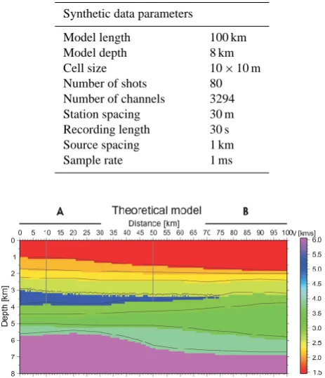
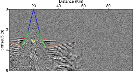
A second order finite difference solver of the elastic wave equation using Sochacki’s interface scheme (Sochacki et al., 1987, 1991) was used to generate a seismic dataset acquired over the velocity model. The 2-D model was of 100 km wide and 8 km deep and a 10×10 m grid was used (Fig. 1). Af-ter intense calculations, 80 shot-gathers were simulated with more than 3000 traces per shot (one trace every 30 m) and 30 s of recording time. The sampling for this synthetic dataset was 1 ms. The parameters for these simulations are sum-marised in Table 2. In this data several phases were identified (Fig. 2). The source wavelet is a minimum phase wavelet with a frequency content of 5 to 25 Hz. Travel time data was picked using the peak amplitude as the reference and an estimated uncertainty of 0.010 s was used in the inversion scheme.

Water multiple and peg-leg signal were generated by the elastic finite difference algorithm, no additional noise was included in the data. Although in nature, basalts appear as highly heterogeneous layered structures, in order to simplify the problem, the basaltic wedge was considered as an ho-mogeneous feature in its internal velocity distribution. Under these conditions we obtained a quite ideal dataset.

Table 2. Parameters used to generate synthetic data.

Synthetic data parameters

Model length 100 km

Model depth 8 km

Cell size 10×10 m

Number of shots 80 Number of channels 3294 Station spacing 30 m Recording length 30 s Source spacing 1 km

Sample rate 1 ms

Fig. 1. Synthetic velocity model resampled using 100×100 m squared cells. The original model used to run simulations was sam-pled by 10×10 squared cells. Vertical lines at 10 and 50 km show the location of hypothetical wells drilled through the basalt layer. Thus at this points, the thickness of the basaltic wedge was known. This information was used in the inversion (see text for more expla-nation).

4 Tomographic inversions

(4)

Fig. 2. Synthetic shotgather. Different phases can be identified: wa-ter wave (blue), refraction from sediments over the basalt layer (green), refraction from basalt (red), reflection from the top of the basalt (yellow), refractions from basement (purple) and reflections from the top of the basement (orange).

in ray paths that would appear when using constant velocity cells ( ´Cervený, 2001). The appendices in Trinks et al. (2005) go to further detail in mathematics used to fill in the veloc-ity grid. Depending on the ray densveloc-ity the algorithm allows for a denser model parametrization of the densely sampled regions, increasing the resolution and efficiency of the algo-rithm. The inversion follows Vesnaver (1994); Böhm (1996) scheme that reduces the non-uniqueness of the travel-time inversion result by adapting the grid.

The forward problem is solved by using an analytical ray tracing in a medium with a linear gradient of slowness squared (Farra, 1990; ´Cervený, 2001), an initial-value ray-tracing scheme with traveltime interpolation is used. The model parametrization and the ray-tracing approach used by this algorithm allow for an efficient analytical computation of the Frechet derivatives of travel-time with respect to model parameters. Trinks et al. (2005) demonstrates that the calcu-lation of the Frechet derivatives are only needed at the points along the ray paths that correspond to the travel-times, not at every point of the model grid. Therefore, the inversion ap-proach is very efficient. Finally, Trinks et al. (2005) demon-strates this points using synthetic and real data tests. Further details on the TTT tomographic algorithm can be found in Trinks et al. (2005).

The final model 3 by this adaptive tomographic inversion scheme was reached when it was able to reproduce the the travel time data within the picking uncertainty andχwas ap-proaching 1. The average velocity structure of the zone over the basalt layer was recovered as well as the top of the basalt layer where a sharp velocity contrast is displayed. However, no low velocity can be reproduced under the basalt, toward the right end of the model, where no basalt exists, some re-alistic information about velocities can be obtained for the deepest part of the model. These results suggest that there are physical limitations in constraining sub-basalt structures by seismic travel time tomography.

10 I. Flecha et al.: Study on the limitations of travel-time inversion applied to sub-basalt imaging

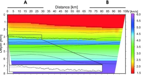
Fig. 3.Velocity model obtained using TTT package Trinks et al. (2005) considering only first arrivals. Interfaces between layers are the ones that were used in the theoretical model. Velocities over the basalt wedge are well constrained. A prominent velocity discontinuity can be observed for the first 70 km between 3 and 4 km in depth which provides the location for the top of basalt layer. A 1 dimensional five layer-cake model was used as the starting model (water, sediments, a wedge of basalt, sediments and basement). Note that the interface between the sediment and the underlying basalt was determined using only the first arrivals. No significant differences in the final model were observed by changing the velocity model 20% in the velocities and 15% in the layer finickinesses. The unresolved parts of the model at both ends of the transect are determined from forward modelling, ray tracing.

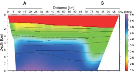
Fig. 4.Velocity model obtained using TTT package Trinks et al. (2005) after inverting refractions from the sediments over the basalt and reflections from the top of the basalt layer. Dashed lines represent layers from inversion and continous lines the theoretical layer interfaces. Note the coincidence between dashed line and continous line in the top of the basalt layer.The unresolved parts of the model at both ends of the transect are determined from forward modelling, ray tracing.

Fig. 3. Velocity model obtained using TTT package Trinks et al. (2005) considering only first arrivals. Interfaces between layers are the ones that were used in the theoretical model. Velocities over the basalt wedge are well constrained. A prominent velocity discontinu-ity can be observed for the first 70 km between 3 and 4 km in depth which provides the location for the top of basalt layer. A 1 dimen-sional five layer-cake model was used as the starting model (water, sediments, a wedge of basalt, sediments and basement). Note that the interface between the sediment and the underlying basalt was determined using only the first arrivals. No significant differences in the final model were observed by changing the velocity model 20 % in the velocities and 15 % in the layer finickinesses. The unre-solved parts of the model at both ends of the transect are determined from forward modelling, ray tracing.

TTT code can also invert additional phases. In order to in-clude all the information from phases identified in synthetic shots, a layer by layer striping inversion was performed. As the problem is a specific one the starting model was cho-sen relatively close to the expected solution to determine if the travel-time data alone was able to resolve the sub-basalt structures, taking into account the high velocity contrasts be-tween the sediments and the basalt. In the seismic exploration area, where this study is applicable, the 1 dimensional aver-age structure is relatively well constrained. Therefore, a rel-atively simple 1-D model was chosen as the starting model. This consists in a five layer cake model these 5 layers corre-spond to: a water layer, a sediment layer, a basalt layer char-acterised by high velocity, and second sedimentary sequence and the basement. So velocities typical of this layers were considered. A series of starting models characterised by a maximum variations of 20 % on the velocity values and 15 % in the thickness where tested with no significant variations in the resolved final models. Top basalt interface was inferred from the model obtained using only first arrivals (Fig. 3). Even though in the theoretical model some sub-layers were included in sedimentary sequences, the contrast in veloc-ity between these sub-layers is quite smooth which makes it difficult to identify events from these interfaces, therefore this minor discontinuities were not considered in the inverted model.

(5)

I. Flecha et al.: Study on the limitations of travel-time inversion applied to sub-basalt imaging 547 10 I. Flecha et al.: Study on the limitations of travel-time inversion applied to sub-basalt imaging

Fig. 3.Velocity model obtained using TTT package Trinks et al. (2005) considering only first arrivals. Interfaces between layers are the ones that were used in the theoretical model. Velocities over the basalt wedge are well constrained. A prominent velocity discontinuity can be observed for the first 70 km between 3 and 4 km in depth which provides the location for the top of basalt layer. A 1 dimensional five layer-cake model was used as the starting model (water, sediments, a wedge of basalt, sediments and basement). Note that the interface between the sediment and the underlying basalt was determined using only the first arrivals. No significant differences in the final model were observed by changing the velocity model 20% in the velocities and 15% in the layer finickinesses. The unresolved parts of the model at both ends of the transect are determined from forward modelling, ray tracing.

Fig. 4.Velocity model obtained using TTT package Trinks et al. (2005) after inverting refractions from the sediments over the basalt and reflections from the top of the basalt layer. Dashed lines represent layers from inversion and continous lines the theoretical layer interfaces. Note the coincidence between dashed line and continous line in the top of the basalt layer.The unresolved parts of the model at both ends of the transect are determined from forward modelling, ray tracing.

Fig. 4. Velocity model obtained using TTT package Trinks et al. (2005) after inverting refractions from the sediments over the basalt and reflections from the top of the basalt layer. Dashed lines repre-sent layers from inversion and continuous lines the theoretical layer interfaces. Note the coincidence between dashed line and contin-uous line in the top of the basalt layer. The unresolved parts of the model at both ends of the transect are determined from forward modelling, ray tracing.

different features within the model. Therefore, a subjective interpretation of the travel time branch is required, and then the picks corresponding to the branch are associated to a par-ticular structure.

4.1 Inverting phases over the basalt layer

Firstly, only the travel time branches interpreted to corre-spond to the sedimentary cover were included in the inver-sion. The results show a good recovery of the original model (Fig. 4). In the first part of the model (thin water layer, 0– 30 km marked as (A) this phase appears as first break and the results are similar to the first arrivals inversion (Fig. 3) while in the last part of the model (thick water layer, 70–100 km marked as (B) the picks used were not considered in first ar-rivals inversion, hence, the additional data provides further constraints on the sedimentary cover over the basalt layer.

The TTT code can include also reflected arrivals in the inversion scheme. As reflections from the top of the basalt are displayed as a very high amplitude events, the travel times of the reflected phases can be identified and picked at normal incidence.

Considering the final model of the previous case as start-ing model, and, without modifystart-ing the velocity values for this model, reflections from the top of the basalt layer were inverted in order to obtain the topography for this interface. A detailed structure was achieved which reproduces in some degree the rugged topography featured by the original model (Fig. 4).

4.2 Inverting refractions inside the basalt

In this case, the main aim is to constrain the base of the basalt using the refracted waves inside this layer. Raypaths

Fig. 5. Results from the basalt refraction inversion. White dashed lines represent layers from inversion and continuous lines the theo-retical layer interfaces. The base of the basalt layer, which is overes-timated, should be delineated by raypaths. The black area represents the part of the model sampled by rays.

are very sensitive to high velocity anomalies, therefore some constraints on the base of the basalt should be gained by in-troducing these refractions. As no noise is present in this syn-thetic dataset, refraction from basalt can be followed up to far offsets (Fig. 2). The maximum offset to stop picking is arbitrary because there is no way to separate basalt refrac-tion from base basalt reflecrefrac-tion. In a first picking stage, re-fractions from the basalt were picked as far as possible and inverted. The results do not fit the theoretical model, overes-timating the basalt thickness (Fig. 5).

(6)

Fig. 6. Synthetic shotgather with noise. Different phases can be identified: water wave (blue), refraction from sediments over the basalt layer (green), refraction from basalt (red), reflection from the top of the basalt (yellow), refractions from basement (purple) and reflections from the top of the basement (orange). Note the differ-ence with Fig. 2 in the refractions from basalt (red).

Fig. 7. Results from the basalt refraction inversion using picks from data with noise. White dashed lines represent layers from inversion and continuous lines the theoretical layer interfaces. The black area represents the part of the model sampled by rays. The base of the basalt layer should be delineated by raypaths. The constrain on the thickness of the basalt layer is failing where the layer is thinner, probably due to overpicking refractions.

4.3 Inverting refractions and reflections from the basement

As shown above, the basalt layer cannot be resolved properly only considering refractions within this layer. In the case of a thicker basalt layer, reflection from the base of the basalt could be differentiated from the basalt refraction which may contribute to better constrain the base of this layer. How-ever, for thin layers there are no possibilities of deducing the basaltic structure using refraction data. At this point, addi-tional information is required to constrain the basalt layer thickness, in a real case, this additional information could be provided by drilling through the basalt layer, fixing in this way the velocity of the basalt, the thickness of the basalt layer and the velocity of the sediments beneath the basalt.

Fig. 8. Final result obtained using all the phases after fixing the base of the basalt layer considering that two wells were drilled through this layer at 10 and 50 km. Dashed lines represent layers from in-version and continuous lines the theoretical layer interfaces. Intro-ducing additional information, the theoretical model is recovered quite accurately. Energy dispersion caused by the topography of the basalt wedge masks the reflected energy from the basement. There-fore, the recovered basement has an irregular top which is not real but the influence of the overlying velocity heterogeneities.

We introduced additional information in the inversion scheme, we assumed that two wells were drilled located at

x=10 km and x=50 km (Fig. 1). In the last part of the model there is no basalt layer, hence the signal coherence is preserved making it possible to identify and pick normal incidence reflections from the basement. Inverting this phase, a reliable estimation of the top of the basement was obtained for the last 25 km of the model which, jointly with the veloc-ity obtained in first arrival inversions, constrained the model in this part. This results were extrapolated under the basalt layer and used as starting model to invert reflections and re-fractions from the basement which yielded to our final model where the theoretical model is reasonably well recovered (Fig. 8). Note that additional information is required by the travel time inversion methods to obtain reliable models.

5 Metropolis simulations

Statistical methods maybe used in order to assess the re-liability of inverted velocity models. Among them, proba-bly Monte-Carlo based simulations are the most used. These consist of generating a relatively large number of random ve-locity models from the same starting model and performing an inversion for each starting model. Finally, the results are compared to asses which model fits the data the best. This method is also used to test the reliability of the starting model in a inversion scheme and the stability of the results (Kore-naga et al., 2000; Sallarès et al., 2003; Martí et al., 2006). In this method every iteration is independent from the previous one and no information is inherited for every new case.

(7)

Table 3. Allowed variation to generate modified models for ve-locity, velocity gradient and thickness for every layer in models 1 and 2.

Layer 1(%)

Water 0

Sediments over basalt 2

Basalt 5

Sediments under basalt 10

Basement 10

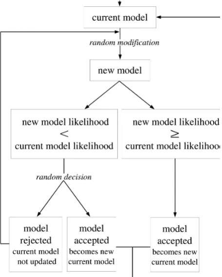
the iterative scheme. In the first stages of the simulation the influence of the starting model is clear but, after some itera-tions, this influence decreases considerably, this is known as “burn-in”. Using this technique the whole region of allowed parameters is visited which yields a random walk within the region of possible parameters. A scheme of the algorithm is shown in Fig. 9 and a detailed description of the methodology can be found in Pearse. In this case, Rayinvr (Zelt and Smith, 1992) was used to solve the forward problem and to calcu-lateχ2which provides the likelihood for every model. The iterative process starts using the starting model (in this case the real model used to build synthetic data) as the current model, then this was randomly modified to generate a new model. Then, the reliability of the model was tested based on the ratio obtained from dividing the likelihood of the current model versus the likelihood of the new model:

– If the ratio was equal or larger than one, the new model was accepted and the new model became the current model.

– If ratio was smaller than one, a random number be-tween 1 and 0 was calculated and another test was per-formed:

– If the ratio was larger than the random number, the new model was accepted and the new model became the current model.

– If the ratio was smaller than the random num-ber, the new model was rejected and the current model remained unchanged.

The process is repeated for a large number of iterations giving as a result a set of different models that reasonably fit the picked travel times when a picking uncertainty is given. In this study, 40 000 iterations were performed for every case in order to obtain a set large enough to have a statistical value. The allowed variations in velocity, thickness and ve-locity gradient were: 0 % for water, 2 % for layer over basalt, 5 % for basalt, 10 % for sub-basalt layer and 10 % for base-ment (Table 3). Variations were chosen increasing in depth to account for the lost of accuracy in deeper layers.

Some synthetic shots have been generated using different 1-D models and two different frequencies 10 Hz and 20 Hz (Figs. 10 and 11):

I. Flecha et al.: Study on the limitations of travel-time inversion applied to sub-basalt imaging 13

Fig. 9.Scheme used in metropolis calculation as described in Pearse (2002). The random modification is subject to prior defined degrees of freedom. In the present case we divide the likelihood of the current versus likelihood of the new model, if ratio is greater than 1 then model is accepted, if ratio is between 0 and 1 then a random decision is taken based on a prior probability function (linear in this case) that will preferentially accept models that are close to the accepted boundary. The likelihood ratio is compared with a normalised random number, if ratio is larger than this number then model is accepted. In any other case, the model is rejected.

Fig. 9. Scheme used in metropolis calculation as described in Pearse (2002). The random modification is subject to prior defined degrees of freedom. In the present case we divide the likelihood of the cur-rent versus likelihood of the new model, if ratio is greater than 1 then model is accepted, if ratio is between 0 and 1 then a random decision is taken based on a prior probability function (linear in this case) that will preferentially accept models that are close to the accepted boundary. The likelihood ratio is compared with a nor-malised random number, if ratio is larger than this number then model is accepted. In any other case, the model is rejected.

– Model 1: model with sub-basalt low velocity layer.

– Model 2: the same as model 1 but with a thicker basalt layer.

5.1 Model 1: results

(8)

Fig. 10. 1-D model used to generate synthetic data (top). Shots gen-erated using the model and different frequencies: 10 Hz (left) and 20 Hz (right). Main phases were identified: sea bottom reflection (blue), top basalt reflection (green), basalt refraction (red), top base-ment reflection (yellow) and basebase-ment refraction (orange). Under the top of the basalt no phases were picked within the water-wave cone because in real data this phases are difficult to identify.

Fig. 11. 1-D model used to generate synthetic data (top). Shots generated using the model and different frequencies: 10 Hz (left) and 20 Hz (right). Main phases were identified: sea bottom reflec-tion (blue), top basalt reflecreflec-tion (green), basalt refracreflec-tion (red), base basalt reflection (purple), top basement reflection (yellow) and base-ment refraction (orange). Under the top of the basalt no phases were picked within the water-wave cone because in real data this phases are difficult to identify.

compared with the identified in the previous case (Fig. 12). Thus, in the first case, we have identified an interference be-tween basalt refraction and base basalt reflection as a pure refraction which is erroneous.

Using the picks from the data obtained with model 1 in the Metropolis approach with a high picking error (see Ta-ble 4) and considering 40 000 different cases, we obtained

I. Flecha et al.: Study on the limitations of travel-time inversion applied to sub-basalt imaging 15

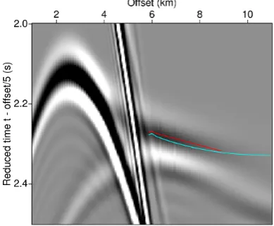
Fig. 12.Basalt refraction picks for model with sub-basalt low velocity layer (red) and for a model without sub-basalt low velocity layer (cyan). In the case without sub-basalt low velocity layer the picks represent a pure refraction while in the other case, the phase that is identified as a refraction is made by the basalt refraction interfering with the base basalt reflection.

Fig. 12. Basalt refraction picks for model with sub-basalt low veloc-ity layer (red) and for a model without sub-basalt low velocveloc-ity layer (cyan). In the case without sub-basalt low velocity layer the picks represent a pure refraction while in the other case, the phase that is identified as a refraction is made by the basalt refraction interfering with the base basalt reflection.

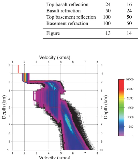
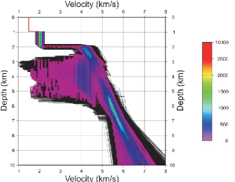
an overestimation in both, velocity and thickness of the sub-basalt layer (Fig. 13). By reducing the picking error (case with low uncertainty) we would expect a better correlation between the more probable model and the theoretical one. In practice, under the same conditions but reducing the picking uncertainty, a worse result was obtained where there was no need of a sub-basalt low velocity layer in order to fit the data (Fig. 14). This effect can be explained because considering a bigger error in the picks, the range of times can include both, refraction within the basalt and reflection from the base of the basalt. Therefore, what was labelled as basalt refraction is within the allowed range of times for this phase. On the other hand, by reducing the picking error, the range of times do not include the real refraction and then our erroneous phase iden-tification yields the unexpected result of Fig. 14.

The same analysis was repeated using model 1 and data generated with 20 Hz. In this case, results are better and fit the right model (Fig. 15).

5.2 Model 2: results

(9)

Table 4. Picking uncertainty in ms for every layer considered in metropolis algorithm.

Phase model1 10 Hz model1 20 Hz model2 10 Hz model2 20 Hz

Seabed reflection 8 8 8 8 8

Top basalt reflection 24 16 16 24 16

Basalt refraction 50 24 24 50 24

Top basement reflection 100 50 50 100 50

Basement refraction 100 50 50 100 50

Figure 13 14 15 16,17 18

Fig. 13. Results obtained after using the Metropolis algorithm on data from model 1 and 10 Hz for 40 000 cases. Red line represents the real model and every black line a modified model. The colour scale stands for the number of times that a model (or part of it) is visited. The preferred model (blue colours) overestimates the sub-basalt layer thickness as well as the velocity for this layer.

cases, sub-basalt velocity layer is not reliably recovered. As in model 1, better fit is obtained for 20 Hz data (Fig. 18), where the velocity gradient for basalt and basement are well reproduced. Again, in both cases, the sub-basalt layer is not well recovered.

The Metropolis study reveals that the phase identification is a critical step. Despite objectivity provided by mathemat-ics used in the inversion, phase identification turns travel time tomography in a subjective procedure. Additionally, un-certainty is also a critical parameter in the inversion which can influence the inversion algorithm. Moreover, consider-ing data with different frequency content also has an effect on the selection of the most probable model. Not all mod-els required a low velocity layer and there was an unresolv-able trade-off between thickness and velocity, even for mod-els where the base basalt reflection could be identified.

Fig. 14. Results obtained after using the Metropolis algorithm on data from model 1 and 10 Hz for 40 000 cases. Uncertainties were reduced in comparison with the previous case (Fig. 13). Red line represents the real model and every black line a modified model. The colour scale stands for the number of times that a model (or part of it) is visited. The preferred model consists in a velocity gradient which includes basalt, and basement layers, avoiding the need of a low velocity layer under the basalt.

Synthetic shots were created using a full-waveform code while likelihood was calculated using a ray tracing code. Full-waveform techniques are more accurate than ray tracing methods because they take into account information about the amplitudes, which are ignored in ray tracing simula-tions. Due to the high computational cost of full-waveform methodologies, ray tracing methods are still conventionally used to obtain velocity models (Pratt et al., 1996). These re-sults suggest that conventional travel time inversion (tomog-raphy) schemes without additional information are not suffi-cient to constrain the base of basalt or sub-basalt geological structures.

(10)

Fig. 15. Results obtained after using the Metropolis algorithm on data from model 1 and 20 Hz for 40 000 cases. Red line represents the real model and every black line a modified model. The colour scale stands for the number of times that a model (or part of it) is visited. The preferred model consists in a velocity gradient which includes basalt, sub-basalt and basement layers. The sub-basalt low velocity layer is reasonably well recovered in velocity and thick-ness.

Fig. 16. Results obtained after using the Metropolis algorithm on data from model 2 and 10 Hz for 40 000 cases considering a “con-servative” picking avoiding picks in the “interference zone”. Red line represents the real model and every black line a modified model. The colour scale stands for the number of times that a model (or part of it) is visited.

Fig. 17. Results obtained after using the Metropolis algorithm on data from model 2 and 10 Hz for 40 000 cases considering more picks than in the previous case (Fig. 16). Red line represents the real model and every black line a modified model. The colour scale stands for the number of times that a model (or part of it) is visited.

(11)

interpreted as results obtained in ideal conditions and in con-sequence, the best ones expected for a real case using this methodology.

6 Conclusions

This study, which involves synthetic data suggests that there are some physical limitations to obtain a reliable velocity model for sub-basalt zones in areas covered by high velocity rocks (like basalts and salts). In the case of thin basalt layers, the base basalt reflection is totally masked within the water-wave cone and it cannot be separated from the basalt refrac-tion. There are several subjective factors that can affect and condition the results from the inversion as maximum pick-ing offset or pickpick-ing uncertainty. Another important point is the frequency content of the signal, our Metropolis simula-tions suggest that the original model is best recovered using high frequencies and thicker basalt. This result is relevant because the actual tendency is using and designing airguns that produce low frequency data as single bubble source. The most critical point in the travel time inversion is the phase identification/interpretation in the shot record. Differentiat-ing in the travel time branch, between the head wave trav-elling within the basalt (refraction) and, the base basalt re-flection is a key element in determining the correct thickness of the basalt. The uncertainty associated to the travel time picks is also a relevant issue, as it can not distinguish be-tween high and low velocity sub-basalt structures. Moreover, a wrong determination of the basalt thickness and velocity has a direct influence on the resulting model for layers un-der the basalt. Reliable sub-basalt imaging with wide-angle reflection/refraction datasets requires additional information as the knowledge on the thickness of the basalt at some point and its internal velocity distribution. This could be achieved by using other methodologies to infer basalt properties.

Acknowledgements. Funding for this research was provided by

SINDRI (Quantitative evaluation of the existing technologies for imaging within basalt-covered areas from the Faroes region), the Spanish Ministry of Science and Technology (Ref: CGL2004-04623/BTE) and Generalitat de Catalunya (Ref: 2005SGR00874). We are grateful to I. Trinks for training in the use of the TTT code.

Edited by: V. Sallares

References

Böhm, G. and Vesnaver, A.: Relying on a grid, J. Seism. Explor., 5, 169–184, 1996.

Carmichael, R. S.: Handbook of Physical Properties of rocks, Vol. II, CSC Press, Boston, 1982.

´

Cervený, V.: Seismic Ray Theory, Cambridge Univ. Press, Cam-bridge, 2001.

Christensen, N. I. and Mooney, W. D.: Seismic velocity structure and composition of the continental crust: A global view, J. Geo-phys. Res., 100, 9761–9788, 1995.

Farra, V.: Amplitude computation in heterogenous media by ray pertur- bation theory: a finite element approach, Geophys. J. Int., 103, 341–354, 1990.

Flecha, I., Martí, D., Carbonell, R., Escuder-Viruete, J., and Pérez-Estaún, A.: Imaging low velocity anomalies with the aid of seis-mic tomography, Tectonophysics, 388, 225–238, 2004.

Fliedner, M. M. and White, R. S.: Depth imaging of basalt flows in the Faeroe-Shetland Basin, Geophys. J. Int., 152, 353–371, 2003. Goff, J. A. and Jordan, T. H.: Stochastic modeling of seafloor mor-phology: inversion of sea beam data for second-order statistics, J. Geophys. Res., 96, 13589–13608, 1988.

Hobro, J. W. D., Singh, S. C., and Minshull, A.: Three-dimensional tomographic inversion of combined reflection and refraction seismic travel time data, Geophys. J. Int., 152, 79–93, 2003. Hobbs, R.: Sub-basalt imaging using low frequencies. Subbasalt

imaging 911th April, 2002 Cambridge, UK Journal of Confer-ence Abstracts, 7, 152–155, 2002.

Hughes, S., Barton, P. J., and Harrison, D.: Exploration in the Shetland-Faeroe Basin using densely spaced arrays of ocean-bottom seismometers, Geophysics, 63, 490–501, 1998.

Jegen-Kulcsar, M. and Hobbs, R. W.: Outline of a joint inversion of gravity, MT and seismic data, Ann. Soc. Sci. Færoensis, 43, 163–167, 2005.

Jolley, D. W. and Bell, B. R.: The evolution of the North Atlantic Igneous Province and the opening of the NE Atlantic rift, Ge-ological Society, London, Special Publication 2002, 197, 1–13, 2002.

Korenaga, J., Holbrook, W. S., Kent, G. M., Kelemen, P. B., De-trick, R. S., Larsen, H. C., Hopper, J. R., and Dahl-Jensen, T.: Crustal structure of the Southeast Greeenland margin from joint refraction and reflection seismic tomography, J. Geophys. Res., 105, 21591–21614, 2000.

Martini, F. and Bean, C. J.: Interface scattering versus body scat-tering in sub-basalt imaging and application of prestack wave equation datuming, Geophysics, 67, 1593–1601, 2002.

Martini, F., Bean, C. J., Dolan, S., and Marsan, D.: Seismic im-age quality beneath strongly scattering structures and implica-tions for lower crustal imaging: numerical simulaimplica-tions, Geophys. J. Int., 145, 423–435, 2001.

Martí, D., Carbonell, R., Escuder-Viruete, J., and Pérez-Estaún, A.: Characterisation of a fractured granitic pluton: P- and s-waves seismic tomography and uncertainty analysis, Tectonophysics, 422, 99–114, 2006.

McCaughey, M. and Singh, S. C.: Simultaneous velocity and inter-face tomography of normal-incidence and wide-aperture seismic traveltime data, Geophys. J. Int., 131, 87–99, 1997.

Metropolis, N., Rosenbluth, A. W., Rosenbluth, M. N., and Teller, A. H.: Equation of state calculations by fast computing machines, J. Chem. Phys., 21, 1087–1092, 1953.

Muir, F. and Dellinger, J.: A practical anisotrophic system., Stanford Exploration Project Reports, 44, 55–58, 1985.

(12)

Pratt, R. G., Song, Z. M., Williamson, P., and Warner, M.: Two-dimensional velocity models from wide-angle seismic data by wavefield inversion, Geophys. J. Int., 124, 323–340, 1996. Pujol, J. and Smithson, S.: Seismic wave attenuation in volcanic 570

rocks from VSP experiments, Geophysics, 56, 1441–1455, 1991. Raum, T., Mjelde, R., Berge, A. M., Paulsen, J. T., Digranes, P., Shi-mamura, H., Shiobara, H., Kodaira, S., Larsen, V. B., Fredsted, R., Harrison, D. J., and Johnson, M.: Sub-basalt structures east of the Faroe Islands revealed from wide-angle seismic and gravity data, Petrol. Geosci., 11, 291–308, 2005.

Richardson, K. R., Smallwood, J. R., White, R. S., Snyder, D. B., and Maguire, P. K. H.: Crustal structure beneath the Faroe Is-lands and the Faroe-Iceland Ridge, Tectonophysics, 300, 159– 180, 1995.

Richardson, K. R., White, R. S., England, R. W., and Fruehn, J.: Crustal structure east of the Faroe Islands: mapping sub-basalt sediments using wide-angle seismic data, Petrol. Geosci., 5, 161– 172, 1999.

Rousseau, J. H. L., Calandra, H., and de Hoop, M. V.: Three-dimensional depth imaging with generalized screens: A salt body case study, Geophysics, 68, 1132–1139, 2003.

Sallarès, V., Charvis, P., Flueh, E. R., and Bialas, J.: Seismic struc-ture of Cocos and Malpelo Ridges and implications for hot spot-ridge interaction, J. Geophys. Res., 108, 5(1)–5(21), 2003. Sava, P. and Biondi, B.: Wave-equation migration velocity

analy-sis. II. Subsalt imaging examples, Geophys. Prosp., 52, 607–623, 2004.

Smallwood, J. R., Towns, M. J., and White, R. S.: The structure of the Faeroe-Shetland Trough from integrated deep seismic and potential field modelling, J. Geol. Soc., 158, 409–412, 2001. Sochacki, J. S., Kubichek, R., George, J. H., Fletcher, W. R., and

Smithson, S. B.: Absorbing boundary conditions and surface waves, Geophysics, 52, 60–71, 1987.

Sochacki, J. S., George, J. H., Ewing, R. E., and Smithson, S. B.: Interface conditions for acoustic and elastic wave propagation, Geophysics, 56, 168–181, 1991.

Sørensen, A. B.: Cenozoic basin development and stratigraphy of the Faroes area, Petrol. Geosci., 9, 189–207, 2003.

Staples, R. K., Hobbs, R. W., and White, R. S.: A comparison between airguns and explosives as wide-angle seismic sources, Geophys. Prosp., 47, 313–339, 1999.

Trinks, I.: Traveltime tomography of densely sampled seismic data, PhD thesis, Cambridge University, 2003.

Trinks, I., Singh, S. C., Chapman, C. H., Barton, P. J., Bosch, M., and Cherrett, A.: Adaptative traveltime tomography of densely sampled seismic data, Geophys. J. Int., 160, 925–938, 2005. Vesnaver, A.: Towards the uniqueness of tomographic inversion

so-lutions, J. Seism. Explor., 3, 323–334, 1994.

White, R. S., Christie, P. A. F., Kusznir, N. J., Roberts, A., Davies, A., Hurst, N., Lunnon, Z., Parkin, C. J., Roberts, A. W., Smith, L. K., Spitzer, R., Surendra, A., and Tymms, V.: iSIMM pushes frontiers of marine seismic acquisition, First Break, 20, 782–786, 2002.

White, R. S., Smallwood, J. R., Fliedner, M. M., Boslaugh, B., Maresh, J., and Fruehn, J.: Imaging and regional distribution of basalt flows in the Faroe-Shetland Basin, Geophys. Prosp., 51, 215–231, 2003.

Williamson, P.: Introduction, Geophys. Prosp., 53, 167–168, 2003. Zelt, C. A. and Smith, R. B.: Seismic traveltime inversion for 2-D

crustal velocity structure, Geophys. J. Int., 108, 16–34, 1992. Ziolkowski, A., Hanssen, P., Gatliff, R., Jakubowicz, H., Dobson,