Simon L Peyton Jones, Chris Clack, Jon Salkild, Mark Hardie
University College London, UK
Abstract
Most MIMD computer architectures can be classified as tightly-coupled or loosely-coupled, depending on the relative latencies seen by a processor accessing different parts of its address space.
By adding microprogrammable functionality to the memory units, we have developed a MIMD computer architecture which explores the middle region of this spectrum. This has resulted in an unusual and flexible bus-based multiprocessor, which we are using as a base for our research in parallel functional programming languages.
In this paper we introduce parallel functional programming, and describe the architecture of the GRIP multiprocessor.
1. PARALLEL FUNCTIONAL
PROGRAMMING
Building a parallel MIMD computer is not a trivial task, but programming it is often more complex still. Functional programming languages provide a particularly promising line of attack, since their freedom from side effects greatly relieves the constraints on parallel program execution. A functional program is executed by evaluating an expression, and several sub-expressions may be evaluated concurrently. For example, in the expression
(3+4) * (sqrt 24)
the addition can take place concurrently with the square root. Thus the hope offered by functional languages is thatparallel execution of functional programs, through concurrent evaluation of sub-expressions, may be possible without adding any new language constructs or detailed program tuning.
If taken without qualification this statement is rather misleading, since it seems to promise "parallelism without tears", whereas in fact co-operation never comes for free. We can, however, take the statement as highlighting an opportunity.
The idea of concurrent execution of programs without adding new language constructs is not new. The FORTRAN compiler for the Cray-1 is designed to spot vectorisable sections of programs written in (almost) ordinary FORTRAN. However, the effective use of the Cray relies on the programmer writing his program in such a way that the compiler can spot that it is vectorisable. Furthermore, high performance is an extremely delicate property of programs, and easily destroyed by seemingly innocuous modifications.
We hope that in the case of functional languages the parallelism is less delicate and more general, so that the programmer’s task is made easier. First, therefore, we will discuss the task of writing parallel functional programs. After this we describe the architecture of GRIP, a multiprocessor designed to execute parallel functional programs.
1.1 Writing parallel functional programs
It is tempting to believe that an arbitrary functional program would run much faster on a parallel graph reduction machine. This comforting belief is quite erroneous; many functional programs are essentially sequential. 1 For example, an insertion sort program cannot insert the next element into the result until the previous insertion has completed (or at least partly completed). It is simply unreasonable to expect any old functional program to run fast on a parallel machine.
computations. Experiments confirm that substantial parallelism is obtainable.21
It is therefore still the program designer’s responsibility to create an algorithm which will divide the task at hand into reasonably independent sub-tasks. It is unreasonable to expect the machine to do this automatically, since it may involve major algorithmic changes (such as changing insertion sort to quicksort).
1.2 Writing parallel programs is easier in a
functional language
Why not program in a conventional language which supports multiple tasks, such as Ada? There are a number of ways in which writing a parallel program in a functional language is superior to this:
(i) In conventional languages the division of the problem into separate tasks is static andfixed. A task is conceived as a relatively large unit, and tasks generally cannot be created and deleted dynamically. There will be relatively few tasks, and the programmer must clearly identify all of them in his design.
In a functional language the parallelism can be dynamic, and there is no static division of the problem into tasks. Instead, the programmer designs an algorithm whose inherent parallelism will enable concurrent reduction to take place at different places in the graph. The "grain" of parallelism is therefore smaller and more dynamically adaptable as the computation proceeds.
(ii) In conventional languages the tasks communicate with each other by sending messages or making specially protected subroutine calls to each other. The programmer has to design synchronisation and communication protocols between tasks so that they cooperate correctly and achieve mutual exclusion where necessary. It is up to the programmer to ensure that these communication protocols are correct, and failure to do so can result in a transient malfunction of the program.
In a parallel functional program, the communication and synchronisation between concurrent activities is handled entirely transparently.
(iii) The tasking structure of conventional languages adds a layer of considerable complexity to the programmer’s model of what is going on. If it is hard to reason about a sequential program, it is even harder to reason about a multi-tasking program, because the programmer has to bear in mind all the possible time orderings in which execution might take place. The behaviour of the program should be independent of the scheduling of the tasks, but it is up to the programmer to ensure that this is the case. Sadly, programming errors frequently have the effect of destroying determinacy, which can make such errors very hard to track down.
There are no extra language constructs required to write parallel functional programs. The result of the program is guaranteed to be independent of the way in which execution is scheduled, though this scheduling may have a strong impact on efficiency. Thus it is no harder to reason about a parallel functional program than a sequential one.
To summarise, the programmer does not have to design a static task structure, guarantee mutual exclusion and synchronisation, or establish communication protocols between tasks. This frees him or her for the creative activity of designing a parallel algorithm.
Naturally, since many of the resource-management and scheduling decisions are now made by the system rather than the programmer, a parallel functional program will probably be less efficient than (for example) an equivalent Occam solution. This is not a new situation; we routinely accept a performance penalty for writing in a high-level language instead of assembly code. Nevertheless, this performance loss and, more seriously, the difficulty of predicting and reasoning about performance, are probably the major shortcomings of parallel functional languages.
Recent developments have been encouraging. Compilers for functional languages are now available for sequential machines which execute programs with performance broadly comparable to compiled Pascal. 34 This technology is now being transferred to parallel machines.
2. EXECUTING FUNCTIONAL
PROGRAMS BY GRAPH
REDUCTION
technique called graph reduction. In this section we offer a brief introduction to graph reduction. A complete treatment can be found in Peyton Jones.5
Consider the following functional program:
let f x = (x+1)*(x-1) in f 4
The "let" defines a function "f" of a single argument "x", which computes "(x+1)*(x-1)". The program executes by evaluating "f 4", that is the function "f" applied to 4. We can think of the program like this:
@
f 4
where the "@" stands for function application. Applying "f" to 4 gives
*
+
-4 1 4 1
We may now execute the addition and the subtraction simultaneously, giving
*
5 3
Finally we can execute the multiplication, to give the result
15
From this simple example we can see that:
(i) Executing a functional program consists of evaluatingan expression.
(ii) A functional program has a natural representation as a tree. As execution proceeds the tree will develop into a graph, because sharing is introduced when function arguments are used more than once in the body of the function.
(iii) Evaluation proceeds by means of a sequence of simple steps, called reductions. Each reduction performs a local transformation of the graph (hence the termgraph reduction).
(iv) Reductions may safely take place simultaneously at different sites in the graph, since they cannot interfere with each other.
(v) All communication between processors performing concurrent reductions is implicit, mediated by the graph. No explicit communication between processors is required.
(vi) Evaluation is complete when there are no further reducible expressions.
Graph reduction provides us with a simple and powerful execution model, that can form the basis of a parallel implementation. The GRIP (Graph Reduction In Parallel) multiprocessor is designed to execute functional programs by performing graph reductions concurrently, exactly as described above. The details of the generation, administration, execution, and synchronisation of concurrent computation are, however, beyond the scope of this paper (see the final chapter of Peyton Jones,5 or Clack and Peyton Jones6 for more details).
3. GRIP SYSTEM ARCHITECTURE
AND PACKAGING
We now turn our attention to the GRIP machine, which has been designed to execute functional programs in parallel. Whilst GRIP was designed for a specific purpose, its architecture has turned out to be quite general, and another group is already engaged in mounting a parallel dialect of Prolog on the same hardware.
Most recent work on MIMD computer architectures has focussed on one of the following areas:
Cache coherence in tightly-coupled bus architectures.
Finding ways of achieving a high degree of locality in a loosely-coupled system.
The GRIP machine explores a different part of the design space, by adding micro-programmable functionality to the memory units.
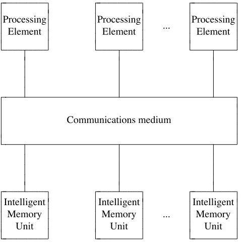
We can think of almost any parallel reduction machine as a variation of the scheme shown in Figure 1. The Processing Elements (PEs) are conventional von Neumann processors, possessing some private memory. The Intelligent Memory Units (IMUs) hold the graph.
Processing Element
Processing Element ...
Processing Element
Communications medium
Intelligent Memory
Unit
Intelligent Memory
Unit
...
Intelligent Memory
Unit
Figure 1. Physical structure of a parallel graph reduction machine
This rather bland-looking diagram actually covers a wide spectrum of machine architectures. The two major axes along which variations are possible are:
The topology of the communications network.
The intelligence of the IMUs.
We now discuss these issues and the decisions we have taken for GRIP.
3.1 The communications medium
In GRIP we have decided to give up extensibility in return for a dramatically improved cost/performance ratio by using a bus as the interconnection medium. The low-level machine architecture is largely centred on the requirement to reduce the bandwidth required from the bus, so as to allow a reasonable number of processors and memories to be connected to it.
The bus architecture is described in more detail below, and is based around the IEEE P896 Futurebus standard.
3.2 The intelligence of the IMUs
The amount of intelligence contained in the IMUs has a radical effect on the architecture. The extremes of the spectrum are:
The IMUs provide only the ability to perform read and write operations to the graph. This results in a classicaltightly-coupled system, where the graph is held in global memory, and every access to the graph by a PE requires use of the communications medium.
The IMUs contain a processor, each sufficiently intelligent to perform graph reduction unaided. The PEs are now vestigial, since they have nothing left to do, and can be discarded altogether.
This results in a collection of processor/memory units connected by a communications medium, which is a classical loosely-coupled system. It is much cheaper for an IMU to access a graph node held in its own local memory than to use the communications medium to access remote nodes.
Though it is seldom pointed out, there is a continuous spectrum of possible architectures between these two extremes. To move from one extreme to the other we may imagine migrating functionality from the PEs into the IMUs.
To the extent that we can be sure of achieving locality of reference, it is desirable to move towards the loosely-coupled end of the spectrum, and to put local processing power in each memory unit. Since small chunks of computation are quite likely to be local, we have chosen to migrate a certain amount of functionality into the memories, by providing them with a microprogrammable processor optimised for data movement and pointer manipulation. This processor is programmed to support a range of structured graph-oriented operations, which replace the unstructured word-oriented read/write operations provided by conventional memories.
Since the IMUs service one operation at a time, they also provide a convenient locus of indivisibility to achieve the locking and synchronisation required by any parallel machine.
These controllers are fundamentally based on the conventional READ/WRITE memory access protocol, and it would be difficult or impossible to adapt them to handle IMUs. It is not at all clear whether the advantages of intelligence in the memories outweighs the disadvantage of not having bus-watching caches, so we regard GRIP as an experiment in this area. One advantage we do have is that our design can be extended to use a more extensible communications network.
Thus, from an architectural point of view, GRIP’s most unusual feature is that it occupies an intermediate point on the closely-coupled/loosely-coupled spectrum. Indeed, depending on the sophistication of the microcode in the IMUs, a range of positions on the spectrum is possible. The IMUs are described in more detail below.
3.3 The Processing Elements
The PEs are Motorola 68020 microprocessors, together with a floating point coprocessor, and as much private memory as we could fit without requiring the microprocessor’s bus to be buffered (128k bytes at present, 1M bytes shortly). In this way, we have capitalised on the extraordinarily dense and cheap functionality provided by microprocessors.
3.4 Packaging
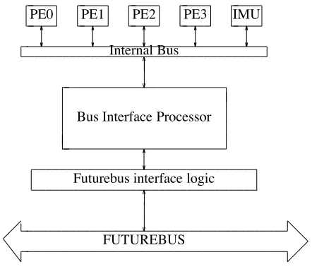
Atfirst we planned to build PEs and IMUs on separate boards, so that we could "mix and match" to find the right ratio between their relative numbers. Subsequently, we realised that the scarcest resource was bus slots, and we should strive to maximise the functionality attached to each bus slot by combining PEs and an IMU on a single board.
It did not seem reasonable or possible to fit more than one IMU on each board, but the PEs are so simple that we are able to fit four of them on each board. Each of these components is connected to the Bus Interface Processor (BIP), which manages their communication with each other and with the bus.
IMU PE3
PE2 PE1
PE0
Internal Bus
Futurebus interface logic Bus Interface Processor
FUTUREBUS
Figure 2. A GRIP board
Figure 2 gives a block diagram of a GRIP board. This (large) single board is then replicated as often as desired, up to a maximum of 21 on a half-metre Futurebus.
An added bonus of this architecture is that communication between a PE and its local on-board IMU is faster than communication with a remote IMU, and saves precious bus bandwidth. The design is not predicated on achieving such locality, but if locality can be achieved it will improve the performance significantly.
3.5 A generic architecture
We designed GRIP specifically to support functional languages, but the machine has in fact turned out to be very general. Through its IMUs, GRIP provides good support for any parallel system with memory-intensive operations, and a separate project is already under way at the University of Essex to mount an OR-parallel dialect of Prolog on the GRIP hardware.7
3.6 Host interfaces
This host (an Orion) provides the development environment for all GRIP’s firmware and software. In addition, each GRIP board is provided with a low-bandwidth 8-bit parallel diagnostics bus, which connects to a custom interface in the Orion. Through this bus all the hardware components on each board can be individually booted up and tested from diagnostic software running in the Orion.
4. BUS ARCHITECTURE AND
PROTOCOLS
In order to use the available bus bandwidth as efficiently as possible, we chose to use a packet-switched bus protocol. This in turn led us to design a packet-switching bus interface, called the Bus Interface Processor (BIP). We now explain the reasons for this choice, and describe the protocol and BIP architecture.
4.1 Packet switching
When using a conventional (circuit-switched) bus protocol, a processor that wishes to read a remote memory locationfirst acquires the bus, then applies the address of the memory location, waits the access time of the memory, and finally reads the data off the bus. During the memory latency, the bus is not in active use, but cannot be used by any other processor. This latency may be relatively long, especially if the memory is intelligent.
In GRIP, therefore, the PE sends an instructionpacketto the IMU, containing details of the operation the PE wishes to be performed, and then relinquishes the bus. While the IMU is processing the packet, the bus is free for other use. When the IMU has completed the operation, it sends a reply packet back to the originating PE.
PE-to-PE, IMU-to-PE and IMU-to-IMU communication is also catered for.
Arbitration for the bus takes place concurrently with data transfer, so when the bus is heavily loaded, very little extra delay is imposed by arbitration. Packet-switching also uses the bus in an efficient block-transfer mode.
4.2 Packet format
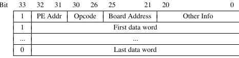
A packet contains one or more words, subject to some
fixed maximum size (currently 256 words). Each word contains 33 data bits, and one "last-word" bit, which is
used to identify the last word of the packet; the packet length is thereby defined implicitly.
The first word of a packet, called the address word, contains routing information, and is interpreted by the BIP; subsequent words are simply transferred without interpretation. In particular, the address word contains the followingfields:
Board Address 5 bits PE Address 2 bits Opcode 5 bits Other info 21 bits
The Board Address uniquely identifies the destination board. If the Opcode is zero, then the destination is a PE, and the PE Address identifies it; otherwise, the destination is the (unique) IMU on the destination board, and the PE address identifies the sending PE. On arrival at the destination board, the BIP automatically replaces the Board Address field with the board address of the sendingboard (which is known to all boards during data transfers).
The effect of these conventions is that it is particularly simple for an IMU to construct the address word of its reply to a PE, because the address word of an incoming request already contains the Board Address and PE Addressfields of the sender.
The Other Infofield is not interpreted by the BIP, but is used in PE-to-IMU transfers to indicate the address of the cell to be operated on; the Opcode indicates the operation to be performed. The packet format is depicted in the Figure 3.
Bit 33 32 31 30 26 25 21 20 0
1 PE Addr Opcode Board Address Other Info
1 First data word
... ...
0 Last data word
Figure 3. Packet format
4.3 The Bus Interface Processor
This buffer memory is divided into a number of fi xed-size packet frames, whose xed-size is a power of two. The memory can then be addressed by supplying a packet address as the most significant address bits, and a sub-packet address as the least significant address bits. There is a (strap-configurable) trade-off between the number of packet frames and their size, but the hardware imposes a limit of 8-bit packet and sub-packet addresses (hence the packet size limit of 256 words).
The BIP also manages an input queue of packets for each PE and the IMU, a queue of packets awaiting transmission over the bus, and a free stack containing empty packet frames. These queues contain packet addresses (not the packet data), which are used to address the packet data held in the buffer memory. Figure 4 gives a block diagram of the BIP organisation:
BUFFER MEMORY
Internal Data Bus Sub-packet address
Temporary Store Free Stack SENDB Queue SENDA Queue IMU Queue
PE3 Queue PE2 Queue PE1 Queue PE0 Queue
(MS address bits) (LS address bits)
Figure 4. BIP block diagram
This organisation confers a number of advantages:
(i) When the board acquires the bus, any packets awaiting transmission can be sent out using the Futurebus’s fast two-edge block-transfer handshake protocol, without the intervention of PEs or IMU.
(ii) If several packets are awaiting transmission (possibly to different destinations), they can be sent out end-to-end, thus amortising the cost of obtaining bus mastership.
(iii) If a PE is sending a packet to the IMU on the same board, or indeed to another PE on the same board, the BIP can simply transfer the packet (address) into the appropriate input queue. The PE sees a single uniform interface.
(iv) Packet addresses can be transferred from one queue to another in the same cycle as they are being used to address the buffer memory. Thus, for example, to send a one-word packet, a PE performs a single memory write cycle to
1. claim a buffer from the Free Stack,
2. load the data into it, and
3. transfer it into the destination queue.
(v) There is considerable scope for ingenuity. For example, the BIP/IMU interface has a small state machine which prefetches the next word which the IMU will require. If the IMU’s input queue is empty, this state machine falls into a "mouth-open" state. When the word it is waiting for is loaded into the BIP’s buffer memory by (for example) the Futurebus receive logic, the state machine spots this fact, and loads the BIP/IMU interface latch with the data word as it goes by. This avoids the latency which would be caused if instead the IMU subsequently acquired BIP mastership and fetched the word out. This sort of thing is only possible because of the un-specialised nature of the internal bus.
There are a few complications. Firstly, when transmitting packets over the Futurebus, the destination board may not have an empty packet frame in which to store the incoming data. In this case, it signals this fact to the source board, which transfers the packet address into the Resend Queue, instead of onto the Free Stack as would be the case for a successful transfer. The Send and Resend Queues swap roles when the send queue has been emptied - hence the titles "SendA" and "SendB" in the diagram.
Secondly, a PE may build a packet in stages, using a number of separate BIP cycles. The Temporary Store provides a place for the packet address to reside while the packet is being built.
4.4 BIP implementation
The BIP is implemented as a fully asynchronous module, built largely out of PALs. It incorporates an asynchronous arbiter to allocate BIP mastership, and uses a simple Go/Done protocol to handshake with the current master.
The Futurebus interface logic, which handles the transmission and reception of packets over the Futurebus, is implemented as two separate asynchronous state machines, which act independently as BIP bus masters. Transmission of data over the bus is pipelined, so that one word can be transmitted over the bus while the next word is simultaneously fetched from the BIP.
5. INTELLIGENT MEMORY UNIT
ARCHITECTURE
The Intelligent Memory Unit is a microprogrammable engine designed specifically for high-performance data manipulation operations on dynamic RAM. In this section we outline the internal architecture of the IMU and the model of the graph which it supports.
5.1 Data representation
The IMUs hold the graph, which consists of an unordered collection ofnodes. Each node is represented by one or more cells, each of which occupies a contiguous area of RAM in the IMU.
The IMU can be programmed to support nodes of either
fixed or variable size. If the node size is variable, then the programmer can choose to represent a node using a linked structure of fixed-size cells, or using a single variable-sized cell. There are many storage management and garbage collection issues here, but the point is that the IMU is sufficiently programmable to allow these trade-offs to be explored.
For the GRIP prototype we have chosen to usefixed-size nodes and cells. To give a more concrete idea of what the IMU is designed to do, we now give the details of this prototype representation. However, it should be emphasised that the representation is largely microprogrammed, so that much of the rest of this section describes firmware decisions rather than hardware constraints.
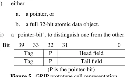
In the prototype representation, each cell contains some tag bitsand twofields- aheadfieldand atailfield(see Figure 5). Afield contains
(i) either
a. a pointer, or
b. a full 32-bit atomic data object.
(ii) a "pointer-bit", to distinguish one from the other.
Bit 39 33 32 31 0
Tag P Headfield
Tag P Tailfield
(P is the pointer-bit)
Figure 5. GRIP prototype cell representation
The cell is stored in two contiguous 40-bit words, each word containing a 33-bit field, and 7 tag bits. The tag information is split between the head and the tail, but since it will be treated as distinct sub-fields (garbage collection mark bits, reference count, cell type, etc), this does not seem to be a problem.
The hardware treats the top 5 tag bits (bits 35-39) specially by allowing them to control 32-way jumps. This allows very fast run-time case-analysis of cell types.
A pointerfield is represented as follows:
Bit 32 31 26 25 21 20 0
1 Flags Board Address Cell Address
This representation is built into the hardware, which has to manipulate pointers directly. The 5-bit Board Address identifies the IMU which holds the cell, and the Cell Address identifies the cell within an IMU. This provides a 64M-cell address space (equivalent to 640M bytes).
The Flags field can be used for any purpose. For example, one bit could be used for a unique reference bit
85one could be used to indicate that the graph pointed to
was already evaluated; and so on. Like the topfive bits of the word, the Flag bits can also be used to drive 32-way jumps, allowing fast case-analysis of the Flagsfield of pointers.
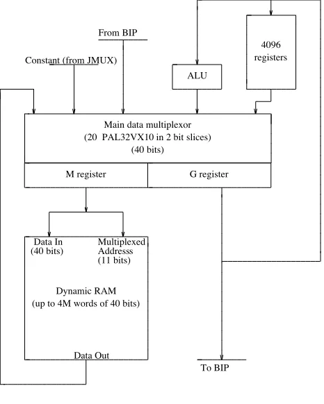
5.2 Data path
the data path around a specially-programmed data multiplexer, built out of PALs, which provides two 40-bit registered outputs. Figure 6 gives the block diagram of the data path.
Dynamic RAM (up to 4M words of 40 bits)
4096 registers
ALU
G register M register
Main data multiplexor (20 PAL32VX10 in 2 bit slices)
(40 bits) Constant (from JMUX)
From BIP
To BIP Data Out
(11 bits)s Address Multiplexed (40 bits)Data In
Figure 6. IMU data path
Taking the ALU off the critical path has allowed us to design to a cycle time of 64ns, and the two output ports of the main multiplexer are extremely useful in overlapping memory operations with other data manipulation. We call the cycle time of the data section atick, to distinguish it from the control section (which cycles at half the speed).
In any tick, the M and G registers can independently be loaded from any of the 5 inputs, or from each other. In addition, a variety of masking operations are available, using a mask stored in the register bank to control the
merge of M or G with one of the inputs.
The register bank consists of 4k 40-bit registers, one of which may be read or written in any tick (but not both). This single-port nature has sometimes turned out to be an awkward constraint in microprogramming, but board area and speed preclude dual-porting them. A large number of registers are provided, because they are often used to hold long constants, thus allowing an 8-bit register address in the instruction to translate to a 40-bit constant.
The "Constant" input is actually driven by a 4-input 5-bit multiplexer (the J mux), whose output is replicated 8 times to cover 40 bits. Using a merge instruction under a mask from a register, a contiguous field of up to 5 bits can thus be inserted in any position in M or G. One input to the J mux is driven by a 5-bit constantfield in the microinstruction; the other three select tag or flag
fields in G and the dynamic memory output.
The 32-bit ALU is built out of two quad-2901 parts, and contains a dual-ported bank of 64 registers internally. It is relatively slow, and is cycled at half the speed of the rest of the data section. Its single input port reflects its lack of importance in the design, and it is up to the programmer to maintain data stable on this port through both ticks of an ALU cycle.
5.3 Dynamic RAM operation
The dynamic RAM is built out of Static Column parts, whose main control signals are Row Address Strobe (RAS), Chip Select (CS) and Write Enable (WE). The IMU is extremely closely-coupled to this RAM. Each tick is divided into threesub-ticksand, for each sub-tick, one bit in the microinstruction controls the state of RAS and CS. The microprogram thus defines a complete waveform for RAS and CS, with a resolution of one sub-tick (21.3ns), which allows the programmer complete freedom to exploit read-modify-write and within-page fast access cycles.
Thisflexibility is a unique feature of the GRIP IMU. It is also extremely simple to implement. The three RAS control bits, for example, are loaded broadside into a shift register at the beginning of each tick, and shifted along every sub-tick; RAS is driven directly off one of the shift register outputs. The CS and WE signals are controlled in a similar way, except that only one bit is needed for WE, because data timing constraintsfix WE inactive during thefirst and last sub-ticks of each tick.
(i) In thefirst tick the row address is supplied from M, RAS is taken active, and simultaneously the two halves of M are swapped over (this is another of the operations provided by the main data multiplexer).
(ii) In the second tick, the column address is now available on the output of M, and CS is taken active.
(iii) Data is available to be read at the end of the third tick, or data can be written, again from M.
Unless a write is taking place, RAS can be taken inactive during the third tick, without prejudicing any read in progress, ready to open an new cell in the next tick. Furthermore, the data just read can be used as the address to be accessed.
If, for example, the program is required to chase down a chain of pointers until some simple condition is met, this design allows the RAM to be cycled in 3 ticks (192ns), which is rather close to the RAM’s specified minimum of 190ns. (The termination condition can, of course, be tested in parallel with accessing the next pointer, since the access can always befinished tidily if the condition is true.)
Of course, life is not always so easy, and in practice a programmer would be lucky to achieve a 100% duty cycle for the RAMs, but the close coupling between program and RAM offers considerable opportunities.
The RAM is protected by parity checking only, and no attempt at error correction is made. Refresh is carried out transparently to the microcode, but holds up the entire IMU while it is happening (less than 1.5% of the IMU’s cycles are lost in this way)
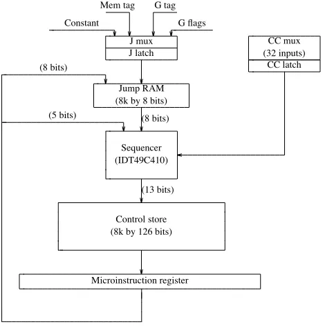
5.4 Control section
The IMU control section is conventional, except that it provides for 16-way and 32-way jumps. Figure 7 gives its block diagram.
Mem tag G tag
(5 bits) (8 bits)
(13 bits) Gflags Constant
(8 bits)
CC latch CC mux (32 inputs)
Microinstruction register Control store (8k by 126 bits)
Sequencer (IDT49C410)
Jump RAM (8k by 8 bits)
J latch J mux
Figure 7. IMU Control Section block diagram
There is one level of pipelining; the condition code (CC) and multi-way jump condition (J) are latched at the end of one cycle and used for conditional branching in the next. The sequencer is an extended 2910, with a 33-deep subroutine stack, and a 16-bit address path.
The control section cycles every two ticks, because it was impractical to make it cycle every tick without an unprogrammable degree of pipelining. It is for this reason that the control store is so wide. It contains a cycle part, which controls the sequencing; and two other parts of identical format, thetick partand thetock part, which control the data section during the the two ticks of the cycle.
provided they all land in the same 256-instruction page. Unconditional jumps are performed by forcing the J latch to zeros, having preloaded the bottom location of each Jump RAM page with the page address, so that the Jump RAM becomes an identity function. 16-way jumps are also provided (to save Jump RAM pages) by forcing the most significant bit of the J latch high or low.
6. PROJECT STATUS AND FUTURE
PLANS
The first wire-wrap prototype is now completed, and is running parallel functional programs. A printed circuit board is in the final stages of layout, and should be completed around the middle of 1988. Meanwhile we have started work on a compiler for GRIP, which should offer greatly improved performance.
6.1 Languages and compilers
GRIP is designed primarily to execute functional languages using parallel graph reduction, and all our software development effort has gone into supporting this aim.
As remarked earlier, a major advantage of programming a parallel machine in a functional language is that no language modifications are required to support parallelism; the parallelism is implicit in the data dependencies of the program. Nevertheless, we augment the language with annotations, which provide hints to the compiler about which parts of the program can be evaluated in parallel. These annotations cannot affect the correctness of the result produced, though they may have a substantial effect on the execution speed. This approach carefully separates the semantics of the program (which concern its correctness) and its pragmatics (which concerns its execution speed), and this separation is a powerful aid in fighting the complexities imposed by parallel execution. The compiler itself also uses a technique called strictness analysis to deduce further annotations. For many programs this may be quite sufficient, so that no programmer annotations are required.
We are currently using the Lazy ML language, from Chalmers University, because we have access to the source code of their compiler, but we expect to move to the new Haskell language shortly. 9 The compiler translates the high-level language program into a functional language intermediate code called FLIC, 10 through which we can support variety of
implementations. Our use of FLIC as an intermediate code ensures that we can use other high-level functional languages fairly easily, by first translating them into FLIC.
6.2 Applications
We have made various claims about the power of parallel functional programming, but these claims can only be substantiated by experience. We are therefore seeking collaborators who have a computationally-expensive application, and who are interested in building an experimental version of it in a parallel functional language. They will need to be prepared to learn a new programming style but will have the opportunity to experience the benefits of rapid execution, on one the world’sfirst powerful parallel graph reduction machines.
The sort of application we are looking for can be characterised as follows:
It should be computationally intensive. We believe that highly parallel algorithms can be developed for almost any computationally intensive problem, even if the standard algorithms are rather sequential.
It should not be I/O bound. Achieving high I/O bandwith has not been the main design aim in our machine.
Examples of possible application areas include:
Numerical modelling (eg Monte Carlo, field equations,finite-element analysis).
Circuit simulation.
Artificial intelligence.
Expert systems.
The higher levels of image analysis.
Computational graphics.
We are setting up a new project, GRASP (Graph Reduction for Application-Specific Programming), to support this application-oriented work. As well as providing the appropriate infrastructure tools, GRASP will run a Technology Support Team, which will provide training and support for the applications partners.
Anyone interested should please contact the authors.
6.3 Present funding and partners
References
1. CD Clack and SL Peyton-Jones, ‘‘Generating parallelism from strictness analysis,’’, Internal Note 1679, Department of Computer Science, University College London (Feb 1985).
2. Steven Tighe, ‘‘A study of the parallelism inherent in combinator reduction’’, MCC Tech Rep PP-140-85, Austin, Texas (Nov 1985).
3. Thomas Johnsson, ‘‘Efficent compilation of lazy evaluation’’, in Proc. SIGPLAN Symposium on Compiler Construction, Montreal (June 1984).
4. Jon Fairbairn and Stuart C Wray, ‘‘Code generation techniques for functional languages’’,
Proc ACM Conference on Lisp and Functional Programming, pp. 94-104 (Aug 1986).
5. Simon L Peyton-Jones, The Implementation of Functional Programming Languages, Prentice Hall (1987).
6. Chris Clack and Simon L Peyton-Jones, ‘‘The four-stroke reduction engine,’’, pp. 220-232 in
Proc. ACM Conference on Lisp and Functional Programming(Aug 1986).
7. TJ Reynolds, SA Delgado-Rannauro, ASK Cheng, and AJ Beaumont, ‘‘BRAVE on GRIP’’, Department of Computer Science, University of Essex (1988).
8. William Stoye, Thomas Clarke, and Arthur Norman, ‘‘Some practical methods for rapid combinator reduction’’, pp. 159-166 in in Proc ACM Symposium on Lisp and Functional Programming(August 1984).
9. Phil Wadler, ‘‘The Haskell Language Definition (draft)’’, Department of Computer Science, University of Glasgow (1988).