Unfolding in particle physics: a window on solving inverse problems

Unfolding in particle physics: A window on solving inverse

problems

Francesco Spanò

1_{Royal Holloway, University of London}

Egham, Surrey, TW20 0EX, United Kingdom

Abstract. Unfolding is the ensemble of techniques aimed at resolving inverse, ill-posed

problems. A pedagogical introduction to the origin and main problems related to unfold-ing is presented and used as the the steppunfold-ing stone towards the illustration of some of the most common techniques that are currently used in particle physics experiments.

1 Introduction

The problem of recovering the “true”, untarnished distribution of the values for a given variable from “smeared”, biased and inefficient observations is common to a variety of fields.

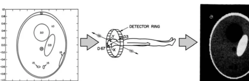
Figure 1 shows an example from medical imaging [ 1]. Positron Emission Topography (PET) aims at visualizing the blood flow and metabolic activity in an organ by introducing a positron-emitting radioactive material (tracer) and by detectingX-ray photons from electron-positron annihilation (e+e− →γγ) when positrons emitted by the tracer annihilate with electrons from the surrounding organic matter. The reconstruction the photon emission spatial density from the detected counts provides the organ’s image and it requires inverting the process outlined in Figure 1.

Images are often blurred by detector effects and corrupted by the presence of additional random noise [2]. Inverting the process shown in figure 2 is necessary to recover the details of initial image.

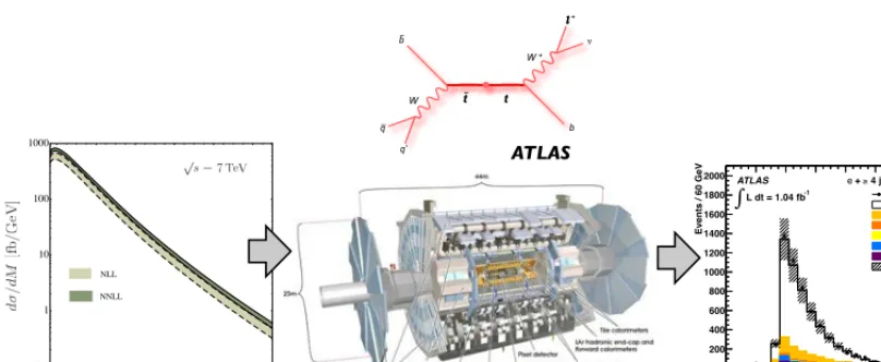
A variety of particle physics measurements share the same “imaging” goal. An illustrative exam-ple is the invariant mass of the pair of top-antitop quarks produced in proton-proton (pp) collisions at a center-of-mass energy (√s) of 7 TeV at the Large Hadron Collider (LHC) [ 3] (pp→tt¯+X) . This is reconstructed by measuring a complex final state involving jets of hadrons and leptons with a multi-purpose detector (in this example the ATLAS detector [ 4]). The inversion of the measuring pro-cess, shown in the cartoon of figure 3, is required to correct for detector (and sometimes acceptance) effects and recover the distribution of the underlying physical property. In particle physicsunfolding

is the ensemble of statistical techniques used to solve what is defined as theinverse problem: infer an unknown distribution f(y) for a variableyfrom the measured distributiong(s) by using knowledge and/or assumptions on the probability distribution that links the observation to the “true” value. Other terms are used that give somewhat more emphasis to recovering one specific feature of the degraded information so the techniques are also namedunsmearingordeconvolving. The proper mathematical formulation of the inverse problem is the crucial step to understand the challenges involved in the unfolding procedure.

DOI: 10.1051/

C

Owned by the authors, published by EDP Sciences, 2013 epjconf 201/ 35503002

Figure 1. Scheme for the evolution of the medical imaging process using figures from Ref. [1]. The simulated

photon pair emission density representing the brain (left, Figure 2) is passed to a simulation of the Positron Emis-sion Tomography (center, Figure 1a) that produces the “observed” count distribution from the photon detector (right, Figure 3a). The names of the figures are as they appear in the reference.

Figure 2. Scheme for the evolution of blurring and degradation of a two dimensional image using figures from

Ref. [2]. The “true” simulated two-dimensional image (left, Figure 4a) is degraded by convoluting it with a Gaussian “spread” function with the addition of random Gaussian noise (see Section 4 in Ref. [2]) to produce the “observed” image (right, Figure 5A). The names of the figures are as they appear in the reference.

2 Unfolding foundations

The mathematical foundations of unfolding are intimately related to the description of the inverse problem [10] provided by the Fredholm integral equation of the first type

g(s)=

ΩK(s,y)f(y)dy (1)

where the true f(y) distribution of the variable y=(y1,..,yJ) is related to the measured or observed

distributiong(s) of the variable s=(s1,..,sL) by the convolution with thekernelfunctionK(s,y) [ 11].

In general the variables y and s belong to multidimensional spaces with different dimensions so the two integersJandLare different, in principle. The “volume”Ωrepresents the support off(y) i.e. the subspace of the multidimensional space where y is defined. The distributionf(y) is transformed into the reconstructed distributiong(s) generally because of limitations in the reconstruction of the data (biases), non-unitary and non-uniform efficiency in their collection and resolution effects.

[GeV] t t m 0 200 400 600 800 1000 1200 1400

Events / 60 GeV

0 200 400 600 800 1000 1200 1400 1600 1800 2000 data t t W+jets Z+jets Diboson Single top Multijets Uncertainty ATLAS -1 L dt = 1.04 fb

1 b tag)

4 jets (

+ e

NNLL NLL

400 600 800 1000 1200 1400 0.1 1 10 100 1000 ATLAS

Figure 3. Scheme of evolution of the measurement of the invariant mass of the top-antitop quark system. The

predicted mass distribution (left, Figure (10, right) in Ref. [5] (shown with the inclusion of theoretical uncertain-ties) for events featuring top-antitop quarks produced in√s=7 TeVppcollisions at the LHC is reconstructed (right, Figure 1(a) from Ref. [6] ) after the top quark decay products are measured by the ATLAS detector (mid-dle, image from Ref. [7] ). A diagram from Ref. [8] shows the final state partons from the top quark decay at leading order. The names of the figures are those by which they appear in the references.

be assessed for consistency, bias, efficiency, and robustness [ 11, 12]. If f(y,a) exists such that it is a

prediction for f(y) expressed as a function of a set of parameters (a1,..,aP), the convolution of f(y,a)

withK(s,y) can be compared with the observed distributiong(s) to extract the parameter vector a

from the data (for instance by means of a fit) and provide a complete description of f(y). However if no parametrized prediction for f(y) exists (as it is often the case), different techniques need to be used to estimate f(y) fromg(s). Operatively the measurements that sampleg(s) are limited in number and affected by biases, inefficiency and imperfect resolution, so a discretized version of the integral equation 1 is used and a limited number of ingredients define the unfolding problem [ 13].

In the very common one dimensional case where bothyandsare real variables, the measured distribution is approximated by the histogram representing the values νi, the expected number of

counts in a given interval ofsaccording to the definition

νi=

si

si−1

g(s)ds (2)

where the interval of definition forsis divided inN sub-intervals by a set of (s1,...,sN) values and

any integral ofg(s) over a specified sub-interval provides the total number of observed events in that sub-interval.

In a similar manner the true distribution is approximated by a histogram. The range of the allowed values foryis also divided inMsub-intervals by a set of (y1,...,yM) values and the expected number

of counts in one of the sub-intervals is defined as

μj=

yj

yj−1

f(y)dy (3)

a value ofsin bini. So Equation 1 is transformed in

νi= M

j₌1

Ri,jμj (4)

whereνiandμjare the expected number of reconstructed and “true” events in binsiandjrespectively.

Consequently the first ingredient for the unfolding problem described by Equation 4 is the knowl-edge of the response matrixR. In generalRis a rectangular matrix and by combining Equation 1 with Equation 2, it is connected to thekernelby the equation

Ri,j=

si si−1

yj

yj−1K(s, y)f(y)dyds

yj

yj−1 f(y)dy

(5)

If the analytical formulation of thekernelis available,Rcan be determined directly from Equation 5. However most frequentlyRis obtained by running detailed simulation of the measuring apparatus including as many effects as possible. Monte Carlo events are generated with the best available pre-diction for the true distributionf(y) and fully simulated with the most accurate model of the detector to produce our best guess ofg(s), the distribution of measured values. For some cases it is possible to measure the response toδ-like (unit-impulse) inputs that can allow to determine thekernelin a certain range of values, like the response of a calorimeter to a beam of particle of known energy and nature. This is equivalent to the integralK(s, y0)=

b

a K(s, y)δ(y−y0)dy.

The second ingredient is the the vector of expected bin contentsννν. The vectorνννis approximated by the vector n=(n1,...,nN) representing the number of observed events in each histogram bin for the

variables. By definitionνννis such thatE[ni]=νiwhereE[ni] indicates the expectation value ofni.

Two additional ingredients are necessary to make the model built in 4 closer to reality.

First some interesting events are not observed due to inefficiencies in the detection or to the re-quirements imposed on the events properties. Such inefficiency is included in the estimate of the response matrixR(i,j) with a proper normalization by defining

Ri,j=

M

j₌1

P(observed in bini|true value in bin j)=P(observed anywhere|true value in bin j)=j

(6) where the vector=(1,..,M) describes the detection efficiency as a function of the histogram bin.

Secondly some of the observed events are not interesting for the measurement one wants to per-form as they are due to backgrounds (events that look like the ones of interest, but have different origin) and they modify the observed distribution. Such events have their own distributionb(s) in terms of the values of the observed variables. The vectorβββof the expected number of background events in each bin of the histogram ofscan be defined as

βi=

si

si−1

b(s)ds (7)

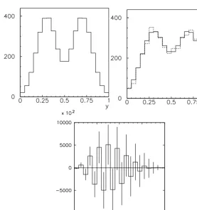
Examples of histograms [13] featuring the vectorsμμμ,and the corresponding vectors n andνννare shown in figure 4.

In general the model described in Equation 1 is then extended to

g(s)=

ΩK(s

Figure 4. Examples of “true” distribution (left) (μμμ), a given set of efficiencies including resolution effects (center) () and the corresponding observed (dashed, right) (n) and expected observed distribution (solid, right)(ννν) [13]. The vectorsμμμ,, n andνννare defined in the text.

and its discretized one-dimensional form described in Equation 4 is consequently extended [13] to

E[ni]=νi= M

j₌1

Ri,jμj+βi (9)

whose vectorial compact form is

E[n]=ννν=Rμμμ+βββ (10)

3 The maximum likelihood solution

Given the problem described by Equation 10, the formal solution is written as

μμμestestest=R−1(ννν−βββ) (11)

whereR−1is the inverse ofR. This estimate forμμμcan also be derived from the principle of maximum likelihood (ML) [14]. If one assumes (fairly generally) that events are being counted in each histogram bin and that the data are consequently independent Poisson observation distributed according to

P(ni|νi)=νn_ii

e−νi

ni!

the logarithm of the global likelihoodL=

N

i=1

P(ni|νi) resulting from the Poisson assumption is

logL(μ)=

N

i₌1

(nilogνi−νi−logni!) (13)

whereννν=ννν(μμμ))) because of equation 10. Consequently the maximum likelihood estimator forννν ob-tained by imposing∂logL(μi)/∂μi=0∀iis given by

νννML=n (14)

and consequently the estimate ofμμμis obtained as

μμμML=R−1(νννML−βββ)=R−1(n−βββ)=μμμest (15)

Is this solution always working ? An example shown in Ref. [ 13] reports a double-peaked true distribution for which the resulting ML estimate, derived according to equation 15, shows a multi-peaked shape with extremely large variances and very large anticorrelation between neighbouring bins: the estimate turns out to be very different from known input. The response matrixRfor this example has sizeable non-diagonal elements and the bin size of the histogram to be “inverted” is smaller than the detector resolution encoded in the model for event migrations. Figure 5 shows the generated “true” histogramμμμ, the observed histogram (dashed) and the corresponding expectation values (solid) and the estimatorμμμestestest.

What is happening? Insight into the reasons for the ML result can be obtained by considering an instance where the trueμμμhave a fine structure and the detection effects, represented by the response matrixR, dilute the true information while allowing residual structure to be present [ 13]. This is shown in figure 6. The application ofR−1aims at restoring the original histogram, according to Equation 15. If the migrations are properly modelled, the inversion returns the correct values if the input data are the expectation vectorνννof the reconstructed bin contents. However the matrix inversion is applied to one instance of the vector n, it is not applied to its expectation valueν. As a consequence, in a suggestively descriptive way,R“assumes” that the fluctuations in n are the residual of a real original structure diluted by the detection effects (and not of statistical origin) and uses the given input and the available model for migrations to reconstructμi.e. it magnifies the fluctuations back into the result.

Independently of the large fluctuations induced by the application of the matrix inversion the maximum likelihood solution is an unbiased estimator ofμμμbecause

E[μμμML]=E[R−1(n−βββ)]=R−1(E[n]−βββ)=R−1(ννν−βββ) (16)

with a covariance given by

UML,i,j=cov[μML,i, μML,j]= N

k,l=1

Ri−,k1R−j,l1cov(nk,nl)= N

k,l=1

R−i,k1R−j,1lδk,lνk= N

k=1

R−i,k1R−j,1kνk (17)

whereδk,l is the Diracδsymbol1 and the equalitycov[nk,nk]=νuses the property of Poisson

dis-tributed data according to equation 12.

Under rather general condition the variance of unbiased estimators has a minimum value (eff ec-tively a lower bound) determined by the Cramér-Rao-Frechet bound [ 14]:

U−min1,k,l=−E[ ∂2_logL

∂μk∂μl

]=

N

i=1

RikRi,l/νi (18)

1_δ

Figure 5. Examples of “true” distribution (left) (μμμ), the observed (dashed, middle) (n) and the expected observed distribution (solid, middle) (ννν) assuming imperfect resolution and perfect detection efficiency, the resulting esti-mate forμμμestusing the ML solution (right) [13]. The vectorsμμμ,ννν, n andμμμestare defined in the text.

If this equation is inverted2 _{the minimum variance equals the ML variance obtained in Equation 17}

i.e. Ui,j=Umin,i,j. Consequently the ML solution provides the unbiased estimator with the smallest

variance. As a consequence estimators providing an additional reduction in variance with respect to the ML estimator will necessarily introduce a bias in the estimate of the true distribution. The balance between bias and variance is a crucial item in the unfolding procedure. Understanding the origin of the large fluctuations in the ML estimator allows to develop techniques to reduce the fluctuations (and consequently the variance of the estimator) while understanding the limitations in terms of bias of the estimator.

4 Correction factors: a “diagonal” ML

A simple step towards a small variance estimator consists in a simplification of Equation 15 derived by taking the same binning forμμμandνννand assumingRto be diagonal (no migrations of events between bins when transforming the true distribution into the measured one). The resulting estimate forμμμis

μi,est=Ci(ni−βi) (19)

Figure 6. Examples of “true” distribution with fine structure (left) (μμμ) and the expected observed distribution (right) (ννν) [13]. The vectorsμμμandνννare defined in the text.

whereCi are correction factors (often called “bin-by-bin corrections”) and they are usually derived

from full simulation of the process under investigation. This provides an estimate for the expected number of reconstructed eventsμ_iMCand true eventsν_iMCand the correction factors are simply derived as

Ci= μMC

i νMC

i

(20)

The corresponding covariance matrix is estimated [ 13] to be

UC,i,j=cov[μMCi , μ MC

j ]=Ci2cov[ni,nj] (21)

The correction factorCi is often of order unity so the variance of the estimators is not much larger

than the Poisson statistical uncertainty in the data and it is typically reduced with respect to the ML estimator uncertainty. In relation to the uncertainties in Equation 21 a simple example due to R. Cousins and reported in Ref. [15]) points out their limitations. If one assumes that, for a given bini

of the distribution to be corrected, the values areCi=0.1,βi=0 andni=100, the estimateμi,Cfor the

expected number of events in this bin is obtained byCini=10 and the associated standard deviation

isCi√ni=1. However this estimate maintains that only 10 of the 100 events that are observed in the

bin are actually belonging to the bin, while the remaining 90 events migrated in from other bins. It is then contradictory to have a measurement with a 10% uncertainty when there are in fact only 10 events that are actually carrying information about the bin content.

The bias corresponding to this technique, defined as E[μi,est]-μi, is estimated [13] to be

b=(μ

MC i νMC

i

− μi νsig

i

)νsi_ig (22)

whereν_isig=νi -βi. The bias b is zero only if the simulation provides a proper description of the

(unknown) true distribution and the bias pulls the result towards the values derived by the model that is used to determine the correction factor.

Ultimately the values ofCidepend circularly on the assumed true distribution one is trying to find.

differently from the ML estimator. The reduction in statistical uncertainty is obtained in exchange for a bias on the estimated result and the actual estimate of the bias is not simple. The bias is reduced if the migration between bins are a small fraction of the bins contents i.e. if the non-diagonal elements of the response matrixRare much much smaller than unity. Another visualization of this reduction is the requirement for the bin width to be large compared to the measurement resolution. Given its limitations in terms of possibly large biases, the technique of correction factors is a good tool for an initial approximation of the results, but it is generally advisable to avoid it for general use 3

5 Back to basics: where to from the maximum likelihood solution?

The sensitivity to fluctuations associated with the ML solution stems from the nature of equation 15 : the original Fredholm equation 1 is an intrinsicallyill-posedorimproperproblem [10] i.e. a problem where“large and sometimes infinite changes in the solution could correspond to small changes in the input data”[16]4_{In this light the stability of the solution of Equation 15 with respect to fluctuations}

can be quantified by how the uncertainties on the inputs are propagated to the output: a quantitative figure of merit for this propagation is the maximum ratio of relative precision of the estimated solution

μμμestof Equation 15 to the relative precision of the measured input vector d=n -βββ, defined as

c(R)=maxd,δd

δμμμest/μμμest

δd/d (23)

The quantityc(R) is called theconditionof theRmatrix and it is the upper bound on the magnification factor for the uncertainties on the input to the inversion. A large value forc(R) implies instability under small fluctuations in the input i.e. a significant sensitivity to “noise” in the measurement.

A deeper analysis of equation 15 illustrates the link between fluctuations and instability and ex-poses the origin of instability in a quantitative manner [ 17] by making a connection with thecondition

of the matrix to be inverted.

The first step is to perform a transformation of variables in equation 15 such that the covariance matrixVdof the vector d becomes the identity matrix. In generalVdcan be non-diagonal as there

can be correlations between the observations in the different bins: the Poisson-based likelihood for independent observations described by Equation 12 is consequently extended to be

L ∝e−12χ

2_(μμμ,d)

=e−12(Rμμμ−d) T_V−1

d (Rμμμ−d) (24)

and the estimates deriving from its maximization coincide with the least squares estimate 5_{. The}

reduction ofVd to the identity matrix allows to write the generalized likelihood of Equation 24 in

terms of significances i.e. variables normalized to their uncertainties. The transformation of variables

3_{A possible exception can be some very well behaved cases with nearly diagonal response matrices where migrations effects}

are minimal, the expected uncertainties are well understood and the expected bias is found to be negligible in comparison to the total final uncertainties on the unfolded results (see also Section13).

4_{A simple and powerful visualization of the ill-posed problem is also given in Ref. [10]: given that thekernelintegration in}

Equation 1 tends to smooth outf(y) and to reduce its high frequency components (edges, cusps and the like), the inversion of such a procedure will inevitably enhance the high frequency features of the input.

5_{In the limit of large expected number of events each independent Poisson variable described in Equation12 tends to}

is a rotation inRN _{followed by rescaling. The matrixV}

dis symmetric and positive definite so there

exists anN×Northogonal matrixQ(QQT _{=1) such thatV}

d=QVdQ

T_andV

dis anN×Ndiagonal

matrix such thatV_d,i,i=v2

i zero andVd,i,j=0 fori j. The new vector dis obtained by a rotation

withQand a rescaling based onvias follows

di =

1

vi N

j₌1

Qi,jdj (25)

The new rotated and normalized dvector encapsulates the statistical significance of the inputs (i.e. their size in units of their uncertainty) : it takes into account the different statistical power of the equation associated to each of the N input values (see Equation 9) . The newRmatrix is also redefined accordingly

Ri,j=

1

vI N

k=1

Qi,kRk,,j (26)

so that equation 11 is reformulated in terms of the new variables as

μμμest=(R)−1d (27)

and the sum of squares to be minimized equivalent to the maximum likelihood is simplified to

1 2χ

2_{(μμμ,d)=(Rμμμ−d)}T

(Rμμμ−d) (28)

The second step is to expose the decomposition of the ML solution in terms of parameters that measure the sensitivity to fluctuations in the input [10]. Such parameters can also be related to the size of the migrations described byR(see Section 4 of Ref. [19]) i.e. the resolution and acceptance performance of the available instruments. This is done by performing asingular value decomposition[ 20] (SVD) ofR. In general a matrixRof dimensionsM×Ncan be decomposed as

R=UΣVT (29)

whereUandVare unitary matrices (UT_U=VT_{V=1)) respectively of dimensionsM×MandN×N}

andΣ = UT_{RV is a diagonal matrix of dimensions M×N i.e. such thatΣ}

i,j=σiif and only ifi

= jotherwise it is zero. Theσivalues are calledsingular valuesof the matrixR, they are non not

negative and can always be arranged in non-increasing order [ 10]. Both matricesU andV can be written in terms of their column vectors: U=(u1,..,uN) andV =(v1,..,vN). IfRis replaced by its

singular value decomposition in the inversion andσj0∀jthe result is

μμμest=(R)−1d=(R)−1(n−βββ)=VΣ−1UTd= N

i=1

1

σi

(uT_id)vi= N

i=1

1

σi

civi (30)

The singular valuesσi have important properties to characterize the unfolded result. The smoother

thekernelcorresponding toR(i.e. the higher order continuous partial derivatives it has), the faster the decay to zero of the singular valuesσiis found to be; the smaller the value ofσibecomes, the

larger the frequency turns out to be for the componentσicorresponds to (i.e. the more oscillations are

present in the functions the correspondingkernelis decomposed in) [ 10]. The coefficientsci=uT_id can

unit-covariance dby the orthogonal matrixUT_{. These normalized coefficients encode the significance}

of the corresponding contribution to the ML result. The contribution of eachciis weighted with the

inverse of the corresponding singular valueσi: small singular values can generate large fluctuations

in the final ML result [21].

The quantitative connection between the singular value decomposition and the magnification of uncertainties in the unfolded result can be found in the conditionc(R) : this can be re-written as

c(R)=||(R)−1δd||/||(R)−1d||/||δd||/||d|| (31)

and it can be shown [22] that

c(R)=||R|| · ||(R)−1||=σmax/σmin (32)

where||d||is the norm of the vector d resulting from the Euclidean positive definite metric inRN_{. For}

the matrixR, the norm||R||is induced by the Euclidean norm. IfA:RN _→RN _{is a linear application}

with the Euclidean norm for a vector||x|| = (ix2i) 1

2 defined for bothRN andRM, the norm of the

matrixAis defined as max eigenvalue ofAT_{A. So theconditionof the matrixRcan be read o}ff_from

its singular value decomposition that is connected to the sensitivity to fluctuations in the unfolding problem.

The overall picture is now clearer. The singular value decomposition gives insight into the unfold-ing problem: ML estimators are sensitive to small effects that can lead to large changes in their values. Once the problem is described in terms of uncertainty normalized variables, the large sensitivity to small fluctuations (i.e. high frequency components, in Fourier-like language) can be derived from the high condition numberc(R) for the response matrix that describes the unfolding problem. In order to pose the problem more properly, it is then necessary to reduce the the impact of the low significance, highly oscillating input components while preserving the information available in the remaining high significance, more stable components. The problem is then said to have been “regularized”. As the ML estimator is unbiased according to the discussion of Section 3, regularization inevitably leads to accepting a certain level of bias in exchange for a reduced variance. The bias is defined as the diff er-ence between the expected value of the unfolded result and the true unmeasured expected value. The heart of unfolding problems lies in understanding the balance between bias and uncertainty.

6 Regularized unfolding: a general view

The likelihood formulation of the unfolding problem in Equations 13 and 24 quantifies the distance between the data vector n and the expectation vectorννν. According to that distance, in a neighbourhood of the ML solution inRN the values ofμμμare such that

logL(μμμ)≥logLmax−ΔlogL (33)

In order to filter out a certain amount of the high frequency components of the input and alleviate the sensitivity to large fluctuations, this distance definition can be modified with the goal to single out a modified solution that is still “close” to the unbiased ML estimate, but less sensitive to fluctuation. A transparent way to carry out such modification is to impose constraints on the initial likelihood by adding Lagrange multipliers and describing the regularization as a maximization procedure for a new likelihoodφ.

The logarithm of the new likelihood to be minimized then becomes

or

φ=logL(μμμ)+τS(μμμ) (35)

whereL(μμμ) is the initial likelihood (for instance from either Equation 13 or Eq. 24),S(μμμ) is called regularization function,αandτare the regularization parameters that allow to tune the strength of the constraints (equivalent a special choice ofΔlogL). In addition, it is possible to add the constraint that

ntot=

N

i=1νiif the solution is required to provide an unbiased estimate of the total number of events.

This results in the maximization of

φ=αlogL(μμμ)+S(μμμ)+λ(ntot− N

i=1

νi) (36)

as a function ofλandμμμ. It should be noted that Ni₌1νiis a function ofμi asνi=Ni₌1Ri,jνj+βi.

The regularization function is often perceived as a measure of the level of “smoothness” required of the maximum likelihood solution. In this light, taking for instance the formulation of Equation 34, if

αis set to zero, the solution is set to the smooth function encoding all the constrains (i.e. available pre-existing information): the shape ofS(μμμ) is imposed as the correct one and the data are ignored. If

αtends to infinity (i.e. αis much larger than any of the other coefficients)S(μμμ) carries no weight in the maximization and the ML solution is re-obtained.

In the explicit formalism the ingredients for the regularization of a given likelihoodL(μμμ) are the regularization functionS(μμμ) and a prescription forαto tune the level of filtering for the high frequency components of the input.

7 Regularized unfolding: the Tikhonov scheme

An analytic and quantitative measure of the smoothness of the unfolding solution is the mean square of thekth derivative proposed by Tikhonov and Arsenin in Ref. [ 23]. The proposed form for the regularization functionS is then

S[f(y)]=

(d

k_f(y)

dyk )

2_{dy (37)}

withkin an integer number. Ifk=2 is chosen, Equation 37 can be approximated by a sum over the numerical estimate of second derivative [24]

S(μμμ)=−

M−2

i=1

[(μi₊2−μi₊1)−(μi₊1−μi)]2 (38)

whereM is the number of values used to describe the regularization function or the number of bins used to provide its discrete description. In matrix notation it is possible to re-writeS(μμμ) as

S(μμμ)=(Cμμμ)T(Cμμμ) (39)

whereC is theM×M matrix that encodes the definition of the second order numerical derivatives (see Section 6 in [19])6.

In the limit of large expected and observed number of events for the distribution of interest the logarithm of the likelihood to be maximized results from combining Equations 24, 34 and 33 into

φ(μμμ, τ)=−1 2χ

2_{(μμμ)+τS(μμμ) (40)}

The combined likelihoodφ(μμμ, τ) is a quadratic function ofμgiven the definition ofχ2_{in Equation 24}

and ofS(μμμ) in Equation 38. Consequently the first partial derivatives with respect toμandτto be solved to minimizeφ(μ, τ) return a system of linear equations.

Similarly to Section 5 the first step is a linear transformation such that the input variables d are normalized to their uncertainties and their new covariance matrix is1∈RN_{(diagonal with unitary}

ele-ments). Consequently the value of−1₂χ2_{(μμμ) takes the form reported in Equation 28. The minimization}

of Equation 40 is then equivalent to finding the solution to the problem represented as

Rμ √_τ

C(μ) =

d

0 (41)

which can also be re-written as

RC−1

√_τ

1) =

d

0 (42)

As third step the productRC−1can be expanded by a singular value decomposition like in Equa-tion 29 and the soluEqua-tion of the problem can be written in terms of such expansion like in EquaEqua-tion 30. The major difference is the presence of theτ-dependent constraint. In order to incorporateτin the solution of Eq. 42, a special linear transformation is performed, called Givens rotation [ 25] : this coordinate transformation sets the lower diagonal block proportional toτto zero while transferring the information about theτvariable to the upper block. In this way the solution can be expressed as a function ofτand of the solution forτ=0 [ 19, 21]. The final result [21] is

μμμest= N

i=1

1

σi

( ˜uTid)˜vi= N

i=1

1

σi

φic˜i˜vi (43)

withφi(τ)=

σ2

i

σ2

i+τ

andRC−1_{is SVD-decomposed asRC}−1_{=UΣ˜ V˜}T_{. The small values ofσ}

iare now

regularized by the presence ofτso that they do not cause large fluctuations. Theτparameter acts like a cut offfor a low pass filter to single out the highest frequencies causing the most rapid fluctuations. Whenσiis much smaller thanτthe coefficientφi(τ) behaves likeσi/τinstead of behaving like 1/σi

(see Equation 30) soφitends to zero instead of tending to infinity and the impact of these “frequencies”

is drastically reduced. It is the additional assumption on the smoothness of the solutions that reduces the importance of the solutions that result from highly oscillating solutions. While theCmatrix is set by the assumption on the derivatives, the value ofτis optimized by the properties of the problem at hand. The choice of the value for theτparameter is discussed in detail in Sections 4.3 and 7 of Ref. [19]. Here we report just the salient concepts. The reduction of the impact of higher-frequency, less statistically significant, more noise-like components is a powerful criterion for the choice ofτ. The significance of each component can be read offfrom the coefficients of equation 43 similarly to the general discussion in Section 5. Reference [19] uses the components of the covariance-normalized, SVD-rotated input vector w defined as

w=U˜d=

N

i₌1

˜uTid (44)

The componentswi of w that are of order unity or less are considered to represent statistically

in-significant contributions and given that the impact of the components ofσilarger thanτis suppressed

according to equation 43, settingτequal to the value ofσ2

meet the chosen criterion. Additional optimization for the choice of the value ofτis possible 7_{, for}

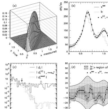
instance by using theτthat gives that best least-squares-based comparison between a generated and the unfolded version fully simulated model for the problem under consideration. Figure 7 shows an “academic” example [19] of unfolding simulated events with this instance of Tikhonov regularization: it reports the response matrix, the superposition of the true, reconstructed and unfolded distributions, the distribution of thewivalues and the difference between the true and the unfolded result. In the

technical implementation of this version for Tikhonov regularization, a correction function is used to scale the simulated truth shape of the truth distribution to obtain the unfolded result. The minimization constraint is actually imposed on the curvature of this shape correction function. As a consequence the normalization information is kept in the response matrix which is no more probability-base like in Equation 4, but it is related to the actual number of simulated events so that the statistical uncertainties on the knowledge of the matrix elements are properly kept into account in the final result.

8 Iterative unfolding

A different approach to including information about the expected true distribution to counter the en-hancement of fluctuations is obtained with an iterative approach.

As pointed out in Ref. [26], the initial idea of an iterative technique for solving ill-posed problems dates back to at least 40 years ago [28]. The general description outlined by Ref. [ 28] provides a still valid basis to understand the core concepts of a large number of the iterative schemes used at present. The inspiration is derived from Bayes’ theorem [ 29] where the sets involved in the formulation are namedobsandtrueto hint respectively at the observed and true number events associated to a given property8_{. In this light Bayes’ theorem can be written as}

P(true|obs)= P(obs|true)f(true)

f(true)P(obs|true)dtrue =

P(obs|true)f(true)

g(obs) (45)

whereP(x|y) is the conditional probability that a variablexhas a certain value given the value of the variableyis betweenyandy+dy,f(x) is a probability density forxandg(obs) is defined as

g(obs)=

f(true)P(obs|true)dtrue. (46)

Inverting equation 45 and using the normalization properties of P(x|y), one obtains

f(true)=

g(obs)P(true|obs)dobs (47)

Equation 47 looks like the “inverse” of 46: it should be noted thatP(true|obs) is actually a function of f(true) itself. The proper inversekernelfor f(true) needs to be a function of P(obs|true) only.

Equation. 45 provides the ansatz that if an initial hypothesis is made onf(true), it is possible to use

P(obs|true) estimated from simulation to evaluateP(true|obs) by definingg(obs) as the convolution of f(true) andP(obs|true). The estimate off(true) can be re-used as initial hypothesis for an updated estimate and the procedure can be iterated. So in the therth_{iterative step, using Equation 46,g}r_(obs)

is defined as

gr

(obs)=

fr(true)P(obs|true)dtrue (48)

7_{The current implementation of the Tikhonov scheme with n=2 used in the ROOT Unfolding framework (RooUnfold) [51]}

only allows to selectτ=s2

Figure 7. All the ingredients and results of an unfolding problem resolved with the n=2 Tikhonov scheme from Ref. [19] (a) The response matrix connecting the true distribution to the measured one by encapsulating the model for the detection performance (b) The superposition of the true distribution (solid curve, labelled

xtest_{), the measured distribution (dotted curve, labelled b) and the unfolded distribution (dots, labelledx}tau_with the choice ofτ =s2

10, the tenth singular value c) The superposition of three versions for the absolute value

of the covariance normalized, SVD-rotated input vector called: the unregularized values (solid, labelled|di|), the regularized values(dashed, labelleddτ_i, for τ=s2

10 ) corresponding to equation 44 w, the arrow points to

and consequently Equation 45 returns

Pr(true|obs)= f

r_{(true)P(obs|true)}

gr_(obs) (49)

Using the ansatz of Equation 47, the estimate Pr(true|obs) is then convoluted with the observed

g(obs)datathat is estimated from data. So a new estimate forf(true), the starting point for the (r+1)th

step, is then obtained by using Equation 49 as follows:

fr+1(true)=

g(obs)dataPr(true|obs)dobs=

fr(true)g(obs)data

gr_(obs) P(obs|true)dobs (50)

The iteration ends at the steprfor which modifications to the value of fr+1_{(true) introduced by}

ad-ditional steps are smaller than a given tolerance value. An equivalent statement is that the iterative scheme converges if there is a steprsuch thatg(obs)data=gr(obs) [28]. The integration in

Equa-tions 50 will tend to remove deviaEqua-tions from unity ing(obs)data/gr(obs) that are present on a large

scale compared to the support ofP(obs|true). On the other hand deviations on a small length scale compared to the support ofP(obs|true) will be tend to be averaged out in the integration. This means that the scheme is sensitive to “long wavelength” errors ingr(obs) that are usually corrected for in the initial iterations by incorporating all the useful information on the dataset. Further iterations will take more and more into account “shorter wavelength” errors more likely deriving from statistical fluctu-ations ing(obs)data: the resulting corrections will tend to matchgr(obs) to those fluctuations rather

than to the properg(obs) value corresponding to the best estimate of f(true).

The discretized version of the iteration technique described in Ref. [ 26] is based on the assumption that the response matrixRis positive definite and the input binned distributionyiin non negative so

that the relation d=n -βββ=Rμμμ(from Section 3) can be inverted iteratively. The starting point is an hypothesis-guess onμμμcalledμμμ0_{to produce the first estimate d}0_=Rμμμ0_{. At ther}th_{step of the iteration}

the estimate for the vector d is

dir= N

j=1

Ri,jμrj (51)

which is the discrete form of 48 with the correspondenceRi,j →P(obs|true),μr_j → fr(true). This

step can be defined "folding" and it corresponds to equation 48. Consequently therth_{estimate ofμμμis}

obtained as in Equation 50 by "integrating" the response matrixRi,jover the updating functiondi/d_ir

μr₊1 j =1/j

N

i=1

Ri,jμrj(di/dri) (52)

where d is the data input vector and corresponds tog(obs)datain Equation 50. The values ofj

repre-sent efficiencies corrections to account for experimental acceptance losses. This step can be defined as the“unfolding” one and it corresponds to equation 50. From Equation 52, the convergence of the iteration is linked to the updating functionyi/yr_i approaching unity: in fact, given the normalization

conditioniR(i,j)=1,yi/yr_i→1 impliesμr_j+1→μr_j. If the uncertainties are Poisson distributed such

an iteration technique is empirically found to converge to the ML solution [ 30].

8.1 Iterative Unfolding: a recent example

is obtained by defining the problem in terms of the relation of “causes” to“effects”. The “causes” are defined as the contentCi of the bins of the given, unknown true distribution distribution one wants

to recover; the “effects” are the contents of the bins of the observed distributionEi. The connection

between the “causes” and the “effects” is obtained by the simulation-derived response matrixP(EJ|Ci),

the probability that a given causeCiresults into a given effectEj(coherently with to the definition of

response matrix in Section 2). The losses due to limitations in the observations are represented by a common“trash” bin and need to be recovered by efficiency corrections, again estimated by simulation. It is emphasized that the variables the iteration estimates are the expected contents of the binsCi, the

probability that a certain fraction of the total events are found in a given bin, not the overall probability for the distributions. So instead of writing Bayes theorem for a given distribution (spectrum) in the form of

P(xC|XE,R,I)∝P(XE|xC,R,I)P(xC|I) (53)

one restarts from the probability of “causes” (i.e. the bin contents) and so each “cell” (i.e. bin content) of the discretized distribution is considered an independent cause of an effect and the probability is written for the bins as

P(Ci|EJ,I)∝P(Ej|Ci,I)P(Ci|I). (54)

With these definitions choosingP(Ci|I) = p0 = 1/M means that the probability content of a given

cause i.e. a bin is a constant over the bins. This does not mean that all spectra have the same probably (it is not a statement on the probability of the distribution), on the contrary it implies a flat, precisely determined initial spectrum and consequently a very strong prior statement that would bias the result if no additional information were used: this is the starting point and the motivation for iterations. Due to this procedure the final estimate for the unfolded distribution is not expressed in terms of a given prior.

The iteration is then such that

P(Ci|Ej,I)∝P(Ej|Ci,I)P(Ci|I). (55)

The first estimate of the number of eventsn(Ci) in the biniof “causes” can be written as

n(Ci)=

1

i NE

j=1

n(Ej)P(Ci|Ej) (56)

This can also be written as

n(Ci)= NE

j=1

Mi,jn(EJ) (57)

with

Mi,j=

P(Ci|EJ,I)P0(Ci)

[

nE

l₌1

P(EJ|Ci)][ nC

l₌1

P(EJ|Ci)P0(Cl)]

(58)

where, in connection with Equation 52,n(Ci) is corresponds toμ1j,n(Ej) corresponds todi,P(Ci|EJ,I)

corresponds toR(i,j),P0(Cl) corresponds toμ0i and the denominator corresponds todi1. The

can be applied. This smoothing is not applied in the last step of the iteration. The iteration is con-tinued until the solution is considered stable. The criterion for stability is dependent on the analysis; one suggested possibility is to quantify the agreement with the previous iteration by means of a least squares test.

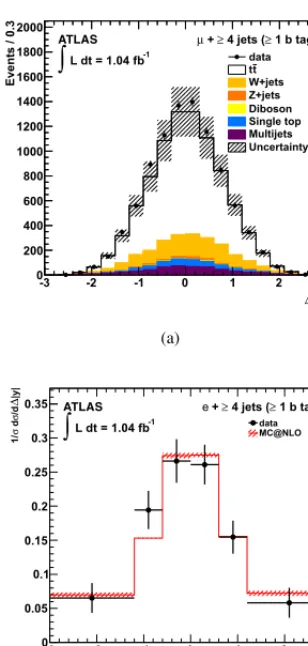
An example from particle physics of the usage of the iterative unfolding technique can be found in the measurement of the distribution of the difference between the absolute rapidities (Δ|yt|) of the

reconstructed top quark and anti-top quark in a sample enhanced intt events obtained by LHC pp

collisions at √s=7 TeV [6]. In the standard model of particle physics this distribution is expected to show a slight asymmetry (at the sub-percent level) in the amount of events with positive and negative differences [6, 32]. The asymmetry is obtained by integrating the unfolded differentialttproduction cross section asΔ|yt|. The migration matrix is shown in figure 8. The measured and unfolded

distri-bution for one specific set of events (featuring a single electron plus jets with at least one b-tagged jet) is shown in figure 8. A set of basic tests are performed to choose the number of iterations, the statistical and systematic uncertainty are propagated through the unfolding scheme and the stability and robustness of the procedure is tested. The number of iterations is such that the expected variation of the value for the asymmetry is stable within 0.1% in simulatedttevents. The statistical uncertainty estimate is determined with simulated experiments and the systematic uncertainty is propagated to both the response matrix and the background. Simulatedttevents are re-weighted so produce diff er-ent samples with different true asymmetry. The analysis is performed on each different sample and the set input asymmetries is then plotted versus the resulting reconstructed asymmetries after unfold-ing to check the linearity of the unfoldunfold-ing procedure. The small biases observed in the reconstructed distributions and the extracted asymmetry are quantified by the largest relative deviation over all the bins and the mean uncertainty-normalized relative difference between true and unfolded values from the pull distributions, respectively. Such values are used to assign additional systematic uncertainties to the unfolded distributions and the final asymmetry.

9 Regularization unfolding and Entropy

Information theory can provide an alternative and deeply meaningful form for the regularization func-tion of equafunc-tion 34. Shannon’s informafunc-tion entropy [ 33] for a given distribufunc-tion is defined as:

H=−

M

i₌1

pilogpi (59)

wherepiis the probability for a given event/system to occur/be in a given subsetiof the available

phase space. The entropyHmeasures the amount of uncertainty represented by the probability distri-bution of a given variable and consequently determines the information content that any observation extracted from that population brings to the observer9_.

When new information about a variable is acquired the gain can be quantified by the change in uncertainty (information) between the initial estimate of the probability distribution for the variable and the new one. As the entropyHmeasures the information change, it is at the basis of the principle of minimum relative entropy (or cross-entropy) [ 34]: if there is not enough information to specify a probability distribution uniquely, a consistent estimator for it is obtained by minimizing

S(μμμ)=H(μμμ)=

M

i μilog

μi i

(60)

9_{An outcome from a distribution with a large Shannon entropy is more useful to the observer as it is less predictable than}

|y|

Δ

-3 -2 -1 0 1 2 3

Events / 0.3

0 200 400 600 800 1000 1200 1400 1600 1800 2000 data t t W+jets Z+jets Diboson Single top Multijets Uncertainty ATLAS -1

L dt = 1.04 fb

∫

(a)

|y|

Δ

Generated

-3 -2 -1 0 1 2 3

|y| Δ Reconstructed -3 -2 -1 0 1 2 3 Simulation ATLAS

1 b tag)

≥

4 jets (

≥ + e (b) |y| Δ

-3 -2 -1 0 1 2 3

|y| Δ /d σ d σ 1/ 0 0.05 0.1 0.15 0.2 0.25 0.3 0.35 data MC@NLO ATLAS -1

L dt = 1.04 fb

∫

(c)

Figure 8. (a) Reconstructed distribution of the difference between the absolute rapidities of top quark and antitop quark (Δ |y|) in top quark pair events observed by the ATLAS detector inppcollisions at√s=7 TeV at the LHC. The observed data are represented by the dots, the predicted amount of events and their breakdown in different sources are shown in the histograms in different colours and illustrated in the legend. (b) Migration matrix from simulated top quark pair events. (c) Unfolded differential cross section for the production of top quark pair events as a function ofΔ |y|(dots) compared with the prediction from the standard model (red histogram). All the plots are taken from reference [6].

whereμμμis the estimator vector for the unknown probability distribution, the indexigoes from 1 to the number of M bins of the distribution andis the reference probability distribution, representing the best knowledge about the true, unknown distribution. This method is used whenever the true distribu-tion is known to be non-negative everywhere. When the only knowledge about the true distribudistribu-tion is its being non-negative and the reference distribution is taken to be a constant over all bins (i=0∀i),

μi that has the minimal distance from the reference, initial estimatei in terms of information, but

respects a given set of constraints.

Additional insight into the use of information entropy is provided in Ref. [ 36] where the minimum relative entropy estimate is interpreted as a maximum likelihood estimate. The negative logarithm of the likelihood for a given set of binned observationnito be compatible with a prior distributioniand

to satisfy the the response matrix constraints (see Eq. 24 is considered. This likelihood is shown to be proportional to the regularization functionS(μμμ) in equation 60 up to a constant term (see Appendix A of [36]). The likelihood for a given set of binned observationni deriving from a true unknown

distributionμito be compatible with a prior distributioniis represented by a multinomial

distribu-tion. The negative logarithm of this likelihood is shown to be proportional to the cross-entropyS(μμμ) in equation 60 up to a constant term (see Appendix A of [ 36]). The distributionμiis connected to the

observed data by the response matrix and the likelihood for this requirement is generally represented by the generalizedL(μμμ) of Equation 24. In the end in the estimate ofμμμminimizing the cross-entropy

S(μμμ, ) with the response matrix constraint corresponds to maximizing the distributionφ(μμμ) in Equa-tion 34, the negative logarithm of the full likelihood for the origin and detecEqua-tion of the observed events, in which the cross-entropyS(μμμ) is interpreted as the regularization function. In addition the interpretation ofS(μμμ, ) as a “prior” p.d.f forμprovides the justification in a Bayesian framework [ 37].

9.1 Automatic Regularized Unfolding

An implementation of the minimum relative entropy principle to provide a the regularization function is present in the Automatic Regularized Unfolding (ARU) [ 38]. This scheme is presently used to perform unfolding for one-dimensional problems. The algorithm does not require any parameter to be tuned, differently from theτparameter for the Tikhonov scheme described in Section 7 or the number of iterations for the iterative techniques illustrated in Section 8.

ARU is a regularized fit. The unfolded distribution to be found,b(x), is parametrized as the sum of flexible and smooth piece-wise, non negative polynomial curves with finite support,bj(x), called

B-splines [39] i.e.b(x)=

j

cjbj(x) where the range of the index jis determined by number of non-zero

derivatives and of grid points that characterize the B-splines chosen for the approximation [ 38]. This solution form is folded with the detectorkernel K(y,x) quantifying the miscalibrations, efficiencies and resolution effects to produce the functionf(y)

f(y)=

K(y,x)b(x)dx=

j

cj

K(y,x)bj(x)=

j

cjfj(y) (61)

An extended maximum likelihood fit [40] of f(y) to the data is then performed by minimizing

L(c)=L1(c)+wL2(c) (62)

In this formulaL1(c) corresponds to the negative logarithm of the overall extended likelihood

functionL1(c)=-log (LstandLnorm). The value ofLstandis

Lstand=K

i

˜

f(yi|c) (63)

whereKabsorbs all the normalization constants, the set ofyiare the observed values for the variable y, ˜f(yi)= f(yI|c)/v(c) andv(c)=

dyf(y)=

j

cjFjwithFj=

dyfj(y). The likelihoodLnormallows

to include the variation of the normalization

Lnorm =v(c)N

e−v(c)

So, by using Equations 63 and 64 and the associated definitions,L1(c) can be written as

L1(c)= −logLstand−logLnorm

=−log(K

i

˜

f(yi|c))−log(v(c)N

e−v(c)

N! )

=−logK−

i

log ˜f(yi|c)−Nlogv(c)+v(c)+logN!

=C−

i

logf_v(yi)

(c) −Nlogv(c)+v(c)

=C−

i

logf(yi)+Nlogv(c)−Nlogv(c)+v(c)

=C−

i

logf(yi)+

j

cjFj

(65)

whereC=−logK+logN! includes constants that can be neglected for the purpose of minimization.

L2(c) is the regularization term based on the relative entropy principle

L2(c)=

b(s)lnb_g(x) (x)dx−

j

cjBj (66)

where the normalizationBj=

bj(x)dxis included. The reference distributiong(x) is chosen to be

uniform while the weightwis determined by minimizing the mean integrated squared error (MIS E) onf(y) (that includes an estimate of the bias)

MIS E(f(y))=

dyE[(f(y)−ftrue(y))2]=

dyV[f(y)]+(f(y)− ftrue(y))2 (67)

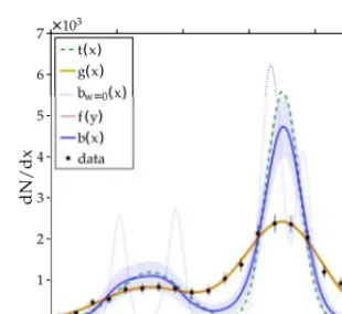
An example of the performance of the technique is shown in figure 9. Unfolding is performed on a sample of one thousand events drawn from a distribution of two Gaussian convoluted with a Gaussian

kernel. The regularized result is compared with the unregularized solution. Figure 10 shows the distributions obtained when performing 2000 simulated experiments with 100 or 10000 events in each experiment, respectively. The uncertainty estimate from ARU is consistent with the observed standard deviation and the average bias has the same size of the statistical uncertainty. A simulation study using 1000 pseudo-experiments of 100 and 1000 events each shows the distribution for the mean and the standard deviation of the unfolded distributions with a bias that is comparable with the statistical uncertainty of the solution.

10 Non-iterative Bayesian-inspired regularization

A non-iterative regularization scheme also inspired by Bayes’ theorem was recently proposed [ 41]. The rationale is to find the probability for the spectrum of a variable as a whole, given the probability for the observed data spectrum and the migration model, according to Bayes’ formula:

p(T|D∧ P)∝P(D|T∧ P)π(T∧ P) (68)

0.0 0.2 0.4 0.6 0.8 1.0 x

0 1 2 3 4 5 6 7

dN

/d

x

×103

t(x)

g(x)

bw=0(x)

Figure 9. ARU-unfolded distribution of a one-dimensional variablexin a simulated experiment using a dataset of 1000 events [38]. The true distributiont(x) is “smeared” into the histogram corresponding to the data points. In this case the folded distribution f(y) used in equation 65 and the reference distributiong(x) used for the regularization in Equation 66 are on top of each other. The regularized solutionb(x) is not showing undesired oscillations, differently from the unregularized solutionbw=0(x).

0.0 0.2 0.4 0.6 0.8 1.0

dN

/d

x

×103

N 100

0.0 0.2 0.4 0.6 0.8 1.0 x

−150 0 150

0 1 2 3 4 5 6 7 8

dN

/d

x

×104

N=10000

0.0 0.2 0.4 0.6 0.8 1.0 x

−4 0 4

×103

Figure 10. Superposed ARU-unfolded distributionsb(x) for a one-dimensional variablexresulting from unfold-ing 1000 pairs of simulated data sets randomly drawn accordunfold-ing to the same true distribution with 100 events (left) and 1000 events (right) fir each pair respectively [38]. The upper plots also superpose the the true distri-butiont(x) on top of the many unfolded solutionsb(x). The bottom plots show the bias of the unfolding defined asb(x)-t(x), the standard deviation (std(b(x)) of the unfolded set of distribution and the median (med(σf it) of the estimated uncertainty on the solution.

is assumed to follow a Poisson distribution of meanRr where R = (R1,RNr) is the Nrdimensional

reconstructed in the reconstructed binr. SoP(r|t) is defined as

P(r|t)= P(t,r)

P(t) =

Mt,r −1

t Nr

k₌1M t,k

(69)

whereMt,r =P(t,r) is the joint probability for an event to be produced in the truth level bintand

in the reconstructed level binrandt is the efficiency for reconstructing events in the bins of rowt

defined as

t= Nr

r=1

P(t,r)

P(t) =

Nr

r=1M tr

P(t) (70)

The interpretation of Equation 68 is that the resultingp(T|D∧ P) is the posterior probability density function (p.d.f.) for the truth level binned spectrum T,P(D|T∧ P) is the likelihood of the observed binned spectrum D as a function of T andPandπ(T∧ P) is the prior p.d.f of T andP.

If the spectrum is such that the data are counts of events, the Poisson distribution can be used

P(D|T)=

Nr

r₌1

Poisson(Dr|T)= Nr

r₌1

RDr r

Dr!

e−Rr ₍₇₁₎

where the mean expected number of eventsRrin a binrof D is

Rr =Br+ Nt

t=1

TtP(r|t) (72)

andBris the expected number of background in binr.

The result of the unfolding is the posterior probability distribution functionp(T|D) for the whole

spectrum. The form of the posterior distribution in Equation 68 is the same as the regularized like-lihood that generates Equation 35 ifL(μμμ) is identified withp(T|D) and if a functionS(T) is defined such that the prior distribution is written as

π(T)=eαS(T) (73)

andS(T) is identified with S(μμμ). Regularization is then interpreted as the inclusion of the prior distribution i.e. the a priori degree of belief in a specified property of the “true” spectrum T. The posterior distributionp(T|D) is used to compute the marginal posterior distributions of the content in

the bins of the spectrumpt(Tt|D) fort∈[1, ...Nt]. Such distributions are defined as

pt(Tl|D)=

..

p(T|D)dT1..dTl−1dTl+1..dTNt (74)

The estimatorTtfor the content of bintof the unfolded spectrum can then be derived by using more

than one algorithm: from taking the mode or the mean of pt(Tl|D) to considering the half point of

the 68% integration interval to using the mean of the Gaussian fitted to thept(Tl|D). The uncertainty

associated with the estimator is usually defined as the shorted interval in the range ofTt for which

the integral of pt(Tl|D) amounts to 0.68. A crucial item for this technique is then the study of the

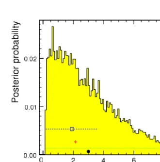
convergence, stability and speed for the integration to be performed in Equation 74 [41]. Figure 11