Probability Distribution Relationships

Probability Distribution Relationships

Yousry H. Abdelkader

and Zainab A. Al-Marzouq

Dept. of Math., Faculty of Science , Alexandria University, Egypt Dept. of Math., Girls College, King Faisal University, KSA.

E-mail address: [email protected] E-mail address: [email protected]

Abstract

—

In this paper, we are interesting to show the most famous distributions and their relations to the other distributions in collected diagrams. Four diagrams are sketched as networks. The first one is concerned to the continuous distributions and their relations. The second one presents the discrete distributions. The third diagram is depicted the famous limiting distributions. Finally, the Balakrishnan skew-normal density and its relationship with the other distributions are shown in the fourth diagram.

Index Term

--

Probability Distributions, Transformations, Limiting Distributions.

I. INT RODUCT ION

In spite of the variety of the probability d istributions, many of them are re lated to each other by different relat ions hips. Deriving the probability d istribution fro m other probability distributions are useful in different situations, for e xa mple , parameter estimations, simu lation, and finding the probability of a certain distribution depends on a table of another distribution. The relationships among the probability distributions could be one of the two classifications: the transformations and limiting distributions. In the transformations, there are three most popular techniques for finding a probability distribution fro m another one. These three techniques are:

1- The cumulative distribution function technique, 2- The transformation technique, and

3- The moment generating function technique.

The main idea of these techniques works as follows: For given functions

g X

i

(

₁

,

X

₂

, ...,

X

n

)

, for

i



1, 2,

,

k

where

the joint distribution of random variables (r.v.'s )

1

,

2

, ...,

n

X

X

X

is given, we define the functions

1 2

(

,

, ...,

),

1, 2, ...,

(1)

i i n

Y



g X

X

X

i



k

The joint distribution of

Y Y

₁

,

₂

, ...,

Y

_n can be determined by one of the suitable method sated above. In particular, for

1

k



, we seek the distribution of

(

)

(2)

Y



g X

For some function

g X

(

)

and a given r.v.

X

.

The equation

(1)

may be linear or non-linear equation. In the case of linearity, it could be taken the form

1

(3)

n

i i i

Y

a X







Many distributions, for this linear transformation, give the

same distributions for different values for

a

_i such as: normal, gamma , chi-square and Cauchy for continuous distributions and Poisson, binomial, negative binomia l for d iscrete distributions as indicated in the Fig. by double rectangles. On

the other hand, when

a

i



1

, the equation

(3)

gives another

distribution, for e xa mp le, the sum of the e xponential r.v.'s gives the Erlang distribution and the sum of geomet ric r.v.'s gives negative- binomial d istribution as well as the sum of Bernoulli r.v.'s gives the binomial distribution. Moreover, the diffe rence between two r.v.'s give another distribution, for e xa mple , the d ifference between the e xponential r.v.'s gives Laplace distribution and the diffe rence between Poisson r.v.'s gives Skellam distribution, see Fig. 1 and 2.

In the case of non-linearity of equation

(1)

, the derived distribution may give the same distribution, for e xa mple, the product of log-norma l and the Beta distributions give the same distribution with different para meters; see, for exa mp le, Cro w and Shimizu (1988), Kotlarski (1962), and Krysicki (1999). On the other hand, equation

(1)

may be give d ifferent distribution as indicated in the Fig..

The other classificat ion is the asymptotic or approximating d istributions. The asymptotic theory or limiting distribution provides in some cases e xact but in most cases approximate d istributions. These approximations of one distribution by another one exist. Fo r e xa mple , for la rge

n

and small

p

the binomial distribution can be appro ximated by the Poisson distribution. Other approximations can be given by the central limit theore m. For e xa mp le, for large

n

The most important use of the relationships between the probability distributions is the simulation technique. Many of the methods in computational statistics require the ability to generate random variables fro m known probability distributions. The most popular method is the inverse transformation technique wh ich deals with the cu mu lative distribution function,

F x

( )

, of the distribution to be simulated. By setting

( )

F x



U

Where

F x

( )

and

U

are defined over the interval

(0,1)

and

U

is a r.v. follows the uniform distribution. Then,

x

is uniquely determine by the relation

1

( )

(4)

x F U





Unfortunately, the inverse transformation technique can not be used for many distributions because a simple closed form solution of

(4)

is not possible or it is so complicated as to be impractical. When this is the case, another distribution with a simple closed form can be used and derived from another or other distributions. For example, to generate an Erlang deviate we only need the sum m exponential deviates each with

expected value

1

m

. Therefore, the Erlang variate

x

is expressed as

1 1

1

ln ,

m m

i i

i i

x

y

U



 





 



Where

y

_i is an e xponential deviate with para meter



, generated by the inverse transform technique and

U

_i is a random nu mber fro m the uniform distribution. Therefore , a complicated situation as in simulat ion models can be replaced by a comparatively simp le c losed form distribution or asymptotic model if the basic conditions of the actual situation are compatible with the assumptions of the model.

Lee mis (1986), Taha (2003) and Ride r (2004) have tried to figure the re lationships amog the probability d istributions in limited atte mpts. The first and second authors have presented a diagra m to show the relat ionships among probability distributions. The diagrams have twenty eight and nineteen distributions including: continuous, discrete and limiting distributions, respectively. The Rider's diagra m div ided into four categories: discrete, continuous, semi-bounded, and unbounded distributions. The diagra m has only twenty distributions. This paper presents four diagrams. The first one shows the relationships among the continuous distributions. The second diagram p resents the discrete distributions as well as the analogue continuous distributions. The third diagra m is concerned to the limiting distributions in both cases: continuous and discrete. The Ba lakrishnan skew-norma l density and its relationships with other distributions are shown in the fourth diagram. It should be mentioned that the first diagra m and the fourth one are connected. Because the fourth diagra m depends on some continuous distributions such as: standard normal, ch i-square, the standard Cauchy, and the

Throughout the paper, the words "diagram" and " fig." shall be used synonymously.

II. THE MAIN FEAT URES OF T HE FIGURES

Many distributions have their genesis in a prime distribution, for e xa mp le, Bernoulli and uniform distributions form the bases to all distributions in discrete and continuous case, respectively.

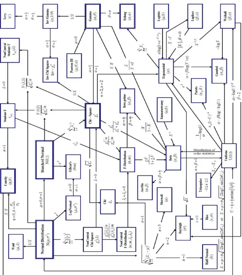
The ma in features of Fig. 1 e xp la in the continuous distribution relationships using the transformat ion techniques. These transformations may be linear or non -linear. The uniform distribution forms the base to all other distributions. The Appendix contains the well known d istributions which are used in this paper and are obtained fro m the following web site: http://www.mathworld.wo lfra m.co m. It is written in the Appendix in concise and compact way. We do not present proofs in the present collection of results. For surveys of this materia ls and additional results we refer to Johnson et al. (1994) and (1995).

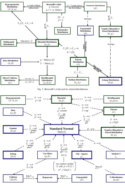
The ma in features of Fig. 2 can be e xpressed as follows.

If

X

₁

,

X

₂

, ...

is a sequence of independent Bernoulli r.v.'s, the number of successes in the first

n

tria ls has a binomia l distribution and the number of failures before the first success has a geometric distribution. The number o f fa ilure before the kth success (the sum of k independent geometric r.v.'s) has a Pascal or negative bino mial distribution. The samp ling without replace ment, the number of successes in the first

n

trials has a hyper-geometric distribution. Moreover, the e xponential distribution is limit of geo metric d istribution, and the Erlang distribution is limit of negative binomia l distribution. The other relationships of discrete distribution as well as the analogue continuous distribution can be seen clearly in Fig. 2.

Fig. 3 is depicted the asymptotic d istributions together with the conditions of limiting. Limit ing distributions, in Fig. 3 and 4, a re indicated with a dashed arrow. The standard norma l and the binomial d istribution play a very predominant role in other distributions.

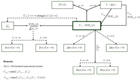
Sharafi and Behboodian (2008) have introduced the

Ba lakrishnan skew-normal density (

SNB

_n

( )



) and studied its properties. They defined the

SNB

_n

( )



with integer

1

n



by

( ; )

( ) ( )

n

(

),

,

,

(5)

n n

f

x





c

 

x





x

x





n





where the coefficient

c

n

( )



is given by





1

1

( )

,

(

)

( )

(

)

n _n

n

c

E

U

x

x dx













 

 



An special case arises when

n



1

and

c

_n

( )





2

which g ives the skew-normal density

(

SN

( ))



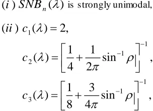
, see Azza lin i (1985).

The probability distribution of the Bala krishnan skew-norma l density and its relationships of the other distributions are also discussed. The most important properties of

( )

n

SNB



are:

( )

i

SNB

n

( )



is strongly unimodal,

1 1 1 2 1 1 3

( )

( )

2,

1

1

( )

sin

,

4

2

1

3

( )

sin

,

8

4

ii c

c

c















   









_



_











_



_





Where



is denoted the correlation coeffic ient. For

4



n

, there is no closed form for

c

_n

( )



. But some approximate values can be found in Steck (1962). The

bivariate case of

SNB

_n

( )



and the location and scale parameters are also presented.

Fig. 4 explains the main features of their results. The dotted arrows indicate asymptotic distribution.

III. CONCLUDING REMARKS

It is a reasonable assertion that all probability distributions are related to one another. In this paper, four diagra ms summarize the most popular re lationships among the probability distributions. The relationships among the probability d istributions are one of the two classificat ions: transformation and limit ing. Each d iagra m e xp lains itself. The advantages of using these diagrams are : the student at the senior undergraduate level or beginning graduate level in statistics or engineering can use the diagrams to supplement course material. Bes ides, the researchers can use the diagra ms for fasting search for the re lationships among the distributions. These diagrams are just start points. Simila r d iagra ms can be constructed to summarize many statistical theorems such as: the characterizat ions of distributions based on; order statistics, Records and Moments, see Gather et al. (1998).

Appendix PDF Parameters Domain Continues Distribution 1 1

(1

)

( )

( , )



_





x

x

f x

B

 

 

0 ,

0









[0,1]

Beta Distribution 1

(1

)

( )

( , )



_

 



x

x

f x

B

  

 

0 ,

0









[0, )



Beta Prime Distribution 2 2

1

( )

(

)







b

f x

x

b





,

0



b





(

 

, )

Cauchy Distribution

 

2 _{1 2}

2 1 1 2

2

( )

  





n x n n

f x

x

e

0



n

[0, )



Chi Distribution

 

1 2 2 2 1 2

( )

2

 





n n x n

x

e

f x

0



n

[0, )



Chi-Squared Distribution 0 0 0

1

,

( )

(

)

0

,









_{ }





x

x

f x

x

x

x

x



0



x

 

x

0

Degenerate Distribution 1 1

( )

(

1)!

x n n

x

e

f x

n





 





1, 2, 3,

,

0

n







[0, )



Erlang Distribution

1

( )

x

f x

e









0





[0, )







1 2 2

2 2 2

1 2

1 2 2

1 1 2 1 2 2 2

( )

,

(

)

 





n n n

n n n n

n n

x

f x

B

n

n x

1



0,

2



0

n

n

[0, )



F- Distribution 1 1

( )

( )

x

x

e

f x

  

 

 





0 ,

0









[0, )



Gamma Distribution

2 (ln ) / 2

1

( )

2





x

f x

e

x



None

(0, )



Gibrat's Distribution

1

( )

            _{ }  _{ }     



x x e

f x

e

   



0 ,







(

 

, )

Gumbel Distribution

2 2_/

2

( )



h

h x

f x

e





0



h

[0, )



Half-Normal Distribution

 

2 ₁

2 1 2

2

2

( )

   





x

f x

x

e

  

0





(0, )



Inverse Chi-Square Distribution

 

1

( )



  



x

f x

x

e



 





0 ,

0









(0, )



Inverse-Gamma Distribution

1 1

( )



a

(1



a b

)



f x

ab x

x

0 ,

0





a

b

[0,1]

Kumaraswamy Distribution

1

( )

2

 



x b

f x

e

b



0,



b



(

 

, )

Laplace Distribution 2 3/ 2

( )

2





c e

c x

f x

x



0



c

[0, )



Levy Distribution 2

( )

1

   _ _    _ _





















x b x b

e

f x

b

e

 

0,



b



(

 

, )

Logistic Distribution





2

2

ln

1

( )

exp

2

2



_



















x

f x

x









0,







[0, )



Lognormal Distribution 2 2 2 2 3

2

( )





x e

x a

f x

a



0



a

[0, )



Maxwell Distribution 2 2 1 2 2 0 2

(

)

( )

2

! (

)

2

         



 



n n x k k n k

x

e

x

f x

k

k





0,

0





n



[0, )



Noncentral Chi-Squared Distribution





 

1 2 1

2 2 2

1 2 1 2 2 1 2 2 1

1 2 1 2

0 0 2 2 ( ) 2 1

( )

2

,

(

)

            











k n l n k n

n n k l n n k l k l k l

n

n

x

f x

e

B k

l

n

n x

 

 

1

,

2

,

1

,

2



0

n n

 

[0, )



 





 



_

_



2 2 2

2 2 2 2

2 2

/ 2 2 2

3 1

1 1 2 2 2( ) 1 1 2 2 2( )

2 1 2

2 ₂

! ( )

2 ( )

2 1; ; 1; ;

( ) ₁

       _{ }     _{ }         n n n n x x n n

n x n x

n _n

n n f x

e n x

x F F

n x _{n x}

   

0,

0





n



(

 

, )

Noncentral Student's t-Distribution 2 2 ( ) 2

1

( )

2

 



x

f x

e

 





2

0,







(

 

, )

Normal Distribution 0 1

( )



_ k k

k x

f x

x

0



0,



0

x

k

0

[

x

, )



Pareto Distribution 1

1

( )

( )

 _     









_

_







x

x

f x

e

 





 



,



0,

 



[0, )



Pearson Type III Distribution 2 2 2 2

( )





x

x e

f x





0





[0, )



Rayleigh Distribution 2 2 2 2 2 2

( )

 







_

_





x o

x

x

f x

e

l











0 ,

0









[0, )



Rice Distribution

2 2

1

( )

2





x

f x

e



None

(

 

, )

Standard Normal Distribution

 

 

1

2 1 2 2 2

( )

(1

/ )













n

n

n

f x

n



x

n

0



n

(

 

, )

Student's t-Distribution

2(

)

(

)(

)

( )

2(

)

(

)(

)





_{ }

 





 

_



_{ }

 





x

a

a

x

c

b

a c

a

f x

b

x

c

x

b

b

a b

c

 

a

c

b

[ , ]

a b

Triangular Distribution

1

( )





f x

b

a

,

a b

[ , ]

a b

Uniform Distribution

1/ 2 ₂

3 2

(

)

( )

exp

2

2















_

_

_

_









x

f x

x

x











0,

0









(0, )



Wald Distribution

1

( )

x

f x

x

e

   





      



,

0

 



[0, )



Weibull Distribution P.M.F. Parameters Domain Discrete Distribution

0

( )

1





 

_



q

x

P x

p

x

0

1,

1

,

 

 

p

q

p

{0,1}

Bernoulli Distribution

(

,

)

( )

( , )

 



 

  

 

n B x

n

x

P x

x

B





 

, 0, 1, 2,   n

 

{0,1,

, }

n

( )

  

 



 

x n x

n

P x

p q

x

0

1,

1

,

1, 2,

 

 



p

q

p

n

{0,1,

, }

n

Binomial Distribution

1

( )



P x

n

1, 2,



n

{0,1,

, }

n

Discrete Uniform Distribution

( )



x

P x

p q

0

1,

1

,

 

 

p

q

p

{0,1, 2,

}

Geometric Distribution

( )











_











 

 

 

Np

Nq

x

n

x

P x

N

n

0,1, 2,

,

0,1,

,

,

0,1,

,

,

,

1









 

N

K

N

n

N

k

p

q

p

N

{0,1,

, }

n

Hypergeometric Distribution

( )

ln(1

)

 



x

P x

x





0

 

p

1

{1, 2,3,

}

Log-Series Distribution

1

( )

1

 





 

_







k x

x

k

P x

p q

k

0

1,

1

,

1, 2,

 

 



p

q

p

k

{0,1, 2,

}

Pascal Distribution

( )

!





x

e

P x

x





0





{0,1, 2,

}

Poisson Distribution

1 2 1 2

1

( )

1

 



 

_



x

P x

x

None

{ 1,1}



Rademacher Distribution





1 2

/ 2

( ) 1

1 2 2

( )



 



_



_

2





x

x

P x

e

 



I

 



1



0,

2



0





{ , 1, 0,1, }

Skellam Distribution

REFERENCES

[1] A. Azzalini, A class of distributions with includes the normal ones, Scandinavian journal of statistics, 12 (1985), 171-178.

[2] E. L. Crow, K. Shimizu, Lognormal distributions: Theory and Applications, Marcel Dekker, New York, 1988.

[3] U.Gather, U., Kampus, and N. Schweitzer, Characterizations of distributions via identically distributed functions of order statistics, In: Balakrishnan, N., and Rao, C. ed., Handbook of Statistics, 16, Elsevier Science, 1998, 257-290.

[4] N. Johnson, S. Kotz and N. Balakrishnan, Continuous univariate distributions, Vol. 1, 2nd ed. Wiley, New York, 1994.

[5] N. Johnson, S. Kotz and N. Balakrishnan, Continuous univariate distributions, Vol. 2, 2nd ed., Wiley, New York, 1995.

[6] I. Kotlarski, On group of n independent random variables whose product follows the beta distribution, Collog. Math. IX Fasc., 2 (1962), 325-332.

[7] W. Krysicki, On some new properties of the beta distribution, Statistics & Probability Letters, 42(1999), 131-137.

[8] L. Leemis, Relationships among common univariate distributions, T he American Statistician, 40(1986), 143-146.

[9] M. Sharafi, J. Behboodian, The Balakrishnan skew-normal density, Statistical Papers, 49(2008), 769-778.

[10] J.W. Rider, Probability distribution relationships,