Improvement in Video Resolution Using
Bayesian Algorithm
1
Sruthi Kurup,
2Dr. S.S. Agrawal
1,2Dept. of E&TC, Smt. Kashibai Navale College of Engineering, Pune, India
Abstract
Videos with super resolution quality are giving its credit to the medical and military fraternity. One such approach is to improve the video quality from high resolution to super resolution (SR). Simply this can be done by using interpolation techniques such as nearest neighbourhood and Bilinear method. But for more appropriate reconstruction, the proposed method can be used. The principle step for it is based on Bayes theorem and an approximation of
symmetric alpha-stable (SαS). It performs maximum a posterior
(MAP) estimation of reconstructed high resolution (HR) image. The heavy tails of the distribution of high resolution image can be captured by the proposed algorithm and hence the edges of the
reconstructed image can be preserved in better way. It removes the
noise from digital images, while the visual quality of the image is
preserved very well. If the received image is in good quality then
automatically the video quality will also improve.
Keywords
Super Resolution; Nearest neighborhood method; Bilinear method; Alpha-stable distributions and Bayesian Algorithm.
I. Introduction
High Resolution (HR) images are at all times essential and requisite
in many military and civilian applications. HR can be defined as
number of pixels within a given size of image and is large in quantity. Therefore, for a variety of practical applications an HR image gives critical information. Petroleum exploration, remote sensing, medical imaging, data mining, military information
gathering and high definition television (HDTV) are the areas
where it can be widely used [3].
To enhance the resolution, there is imperative need for developing post-acquisition signal processing techniques. These techniques
offer flexibility and there is no additional hardware involved, so adds cost benefice. However, a user has to suffer an increased
computational cost that may be the burden. This resolution enhancement is called super- resolution (SR) image reconstruction.
In SR reconstruction, an HR image is restored by using a video
sequence or several LR images. By using optical devices, noises are eliminated and blurs. The size is limited by using embedded sensor chips. To increase the resolution of a sequence of degraded images has engrossed extensive attention of researchers in the
field of computer vision and machine learning.
This paper is organized section wise and is as follows: In Section II, all preliminary works are mentioned. Section III deals with two
approaches of reconstruction: Nearest neighborhood and Bilinear
method. Section IV gives the information about the alpha-stable
distribution and Section V is about Bayesian algorithm. Finally,
Section VI produces all the results and discussions related to it.
II. Literature Survey
In the last few decades, our lifestyle has changed enormously due
to the development of the image and video technology. This has made many popular SR reconstruction algorithms which can be roughly divided into two categories:
Frequency domain algorithms and 1.
Spatial domain algorithms. 2.
Tsai and Huang [4] proposed the first work for the SR reconstruction
by estimating the relative shifts between observations. Their approach is called frequency domain algorithms and is based on the following three aspects: the property of shifting of Fourier transform, the spectral aliasing principle, and the limited bandwidth of the original HR image. Based on this algorithm, a series of improved SR reconstruction algorithms had been proposed [5-6].
For spatial domain algorithms started with non-uniform interpolation-based approach whose computational cost is relatively low so they are ready for real-time applications. However, degradation models are not applicable in these approaches if the blur and the noise characteristics are different for LR images. Projections on a convex set (POCS) based methods have common advantage of simplicity, i.e., the utilization of the spatial domain observation model and inclusion of a priori information. However, their disadvantages are non-uniqueness of solutions, slow
convergence rate and heavy computational load. Iterative back projection (IBP) based approaches conduct SR reconstruction in
a straightforward way.
Christopher R. Dance and Ercan E. Kuruoglu proposed that stable
distribution has proved to be strong alternatives to the Gaussian
distribution. Most of the real life signals are skewed. Closed
form estimates that characteristic function techniques yield the
parameters which may be efficiently computed. Weighted sums of stable variates can be applied to find the skew and location
parameters. [3] An important property of Gaussian Random Variable is that the sum of two of them is itself a Normal Random Variable.
Jin Chen, Jose Nunez-Yanez, and Alin Achim investigated the
increasing problem of spatial resolution of video frames. It is done by using three prior models: GMRF (Gaussian Markov Random
Field), BTV (Bilateral Total Variation) and GGMRF (Generalised
Gaussian Markov Random Field). GGMRF preserves sharp edges
of image in a better way. [4]
Xuelong Li, Yanting Hu, Xinbo Gao, Dacheng Tao and Beijia
Ning proposed a new multiframe SR reconstruction algorithm which is based on image local characteristics. Locally adaptive bilateral total variation model is used as regularization parameter
to balance noise suppression. It introduces a gradient error which
is used as gradient consistent constraint [5].
III. Interpolation Techniques
Super Resolution (SR) technique is method of constructing HR frame from several LR frames. The main idea behind it is to combine the non-redundant information contained in multiple LR Frames to generate a HR image. The closely related technique
the size of the frame increases. But there will be no additional information. Hence the quality of single frame will be very much
limited. It cannot be recovered easily because of lost frequency components. Here we took the cases of nearest neighborhood
and bilinear method.
The nearest neighborhood method is very simple and requires less
computation as it use nearest neighbor’s pixel to fill interpolated
point. This method is just copies available values, not interpolate values as it doesn’t change values.
In bilinear method, interpolated point is filled with four closest pixel’s weighted average. In this method we performed two linear
interpolations, in horizontal direction and then linear interpolation
in vertical direction. It is required to calculate four interpolation functions for grid point in Bilinear Interpolation. It is used to know values at random position from the weighted average of the four closest pixels to the specified input coordinates, and assigns
that value to the output coordinates. The two linear interpolations are performed in one direction and next linear interpolation is performed in the perpendicular direction.
Consider an image of size 2X2 and is in figure 1.
2 3 4 5
Fig. 1: 2X2 Image
As per nearest neighborhood technique, the new image is shown
in figure 2.
2 2 3 3 2 2 3 3 4 4 5 5 4 4 5 5
Fig. 2: Nearest Neighborhood Image
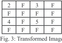
With filler the bilinear method image will turns into an image as shown in figure 3.
2 F 3 F
F F F F
4 F 5 F
F F F F
Fig. 3: Transformed Image
Thus for every F, calculate the mean of the surrounding pixels.
Eventually, you will be able to calculate the mean for every F,
even those that were originally surrounded by all F.
2 F 3 F F F 4 F 5
Fig. 4: Bilinear Image
Eventually, the middle F in fig. 4 should calculate out to being
(2+3+4+5)/4=14/4.
IV. Alpha-Stable Distributions
New statistical approach will deal with alpha-stable model which will be used as learning model. Stable distributions are a rich
class of probability distribution that allow skewness and heavy
tails and have many interesting mathematical properties. Stable distributions have been proposed as a model for many types of
physical and economic systems. It is also used to characterize
wavelet coefficients of natural images. Since the wavelet
coefficients are symmetric in nature, it should be modeled first.
Therefore we restrict our self to the case of symmetric alpha-stable distributions.
A general alpha-stable distribution is specified as S (α, β, c, ). It
is determined using four parameters. The four parameters are as follows:
Shape parameter α (also known as characteristic exponent).
1.
Most important parameter of a stable distribution.
•
The smaller the characteristic exponent α, heavier the tails •
of the SαS density
Skewness parameter β is in [−1, 1] and measures the asymmetry
2.
of the distribution.
Scale parameter, c indicates the width 3.
Location parameter
4. indicates the location of the distribution.
Characteristic function of one-dimensional α-stable distributions
can be described as in equation 1:
Φ (z) = exp (-c [1 + j β sign(z) tan( )] + j (1)
for characteristic exponent α (0, 1) U (1, 2), symmetry parameter
(skew) β [-1, 1], dispersion c > 0 and location parameter
(-1, 1). Do not consider the cases α = 1, 2 where the distribution has special behaviour. Such α-stable distributions have proved to
be strong alternatives to the Gaussian distribution.
A. Univariate Symmetric Alpha-Stable Distributions The two main theoretical reasons for alpha-stable distributions to be used as a statistical model are:
Stable random variables satisfy the stability property. Stability 1.
property states that the linear combinations of jointly stable variables are indeed stable. Stability is nothing but the shape of the distribution remains unchanged (or stable) under such linear combinations.
Stable processes arise as limiting processes of sums of 2.
independent identically distributed (i.i.d.) random variables using the generalized central limit theorem. The distribution
lacks a compact analytical expression for its probability
density function (pdf).
Consequently, it is most conveniently represented by its characteristic function as given in equation (2):
Φ (z) = exp (-c + j µ z) (2)
where α is taking values 0 , - and c > 0 for the
above the distribution. The characteristic exponent (α) is the most important parameter of the SαS distribution, as it determines the shape of the distribution. For values of α in the interval (1-2], the
location parameter µ corresponds to the mean of the distribution, while for 0 , µ corresponds to its median. The dispersion parameter (c) determines the spread of the distribution around its location parameter, similar to variance of Gaussian distribution [1].
B. Bivariate Stable Distributions
of univariate stable distributions. Bivariate stable distribution is
distinct from univariate stable distribution by a single reason. It forms a nonparametric set, therefore, more difficult to describe.
Characteristic function for bivariate stable distributions can be stated in equation (3) and is as follows:
Φ ( ) = exp (-c + j ( (3)
The distribution is isotropic with respect to the location point ( . The two marginal distributions of the isotropic stable distribution are with parameters ( and Bivariate isotropic Cauchy and Gaussian distributions are special cases and can be represented as and respectively.
The bivariate pdf in these two cases are given in equation (4).
for
(4)
As in the case of the univariate density function, when and , no closed-form expressions exist for the density function of the bivariate stable random variable [1].
V. Bayesian Algorithm
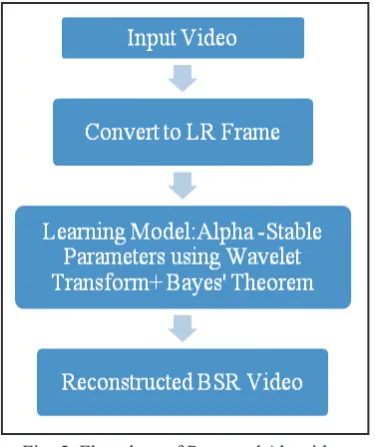
The proposed algorithm transforms the input video to newly
reconstructed video. The flowchart as shown in fig. 5 gives the
generalized idea behind the algorithm.
Fig. 5: Flowchart of Proposed Algorithm
Classical three-step technique can be used for video reconstruction using Bayesian method:
Convert the true frames to Low Resolution (LR) frames. 1.
Learning model will be designed. 2.
Apply Bayes’ theorem. 3.
A. Bayes Theorem Implementation
The wavelet transform is a linear operation. After decomposing an image into six sub-bands consequently and for every two adjacent
levels, sets of noisy wavelet coefficients represented as the sum
of the transformations of the signal and the noise [2] are given as in equation (5).
(5) where 1 refers to the decomposition level.
Equation (6) is the vectorial form of above set of
equations and can be written as
y = x + n (6) where y= ( , x= , n= ( .
The MAP estimator of given image, the noise observation can be easily derived as follows:
= P ( ) (7)
Using Bayes’ theorem, equation (7) can be written as:
= (x)
(x) (8)
Additionally, the shrinkage of a coefficient is also conditioned using equation 8. The shrinkage is done on the value of the corresponding coefficient at the next decomposition level (parent value); the smaller the parent value, the greater the shrinkage [1].
B. Estimation of Parameters
The reconstructed frame can be estimated using the parameters
such as PSNR and SSIM. Peak Signal to Noise Ratio (PSNR)
widely used for measuring the quality of reconstructed image.
Logarithmic scale is used for measuring PSNR. It is defined as
ratio of maximum possible power of image data and power of noise
is the error introduced by compression that affects the fidelity of
its representation.
Usually high PSNR represents high quality of reconstructed image while low PSNR represents low quality of reconstructed image.
It is calculated as written in equation 9:
(9)
where is the maximum possible pixel value of frame.
Apart from measuring the PSNR, the structural similarity (SSIM)
is also used to measure the reconstruction quality [1]. Compared
with the more traditional PSNR, SSIM has been proven to be more consistent with human eye perception. The SSIM is given
in equation 10.
(10)
where are the mean values, and are their variances, and is the covariance. = = are two variables
used to stabilize the division with weak denominator, where L is
the dynamic range of the pixel values and = 0.01, = 0.03
by default. The SSIM measure should be close to unity for an
optimal effect of SR reconstruction [1].
VI. Results and Conclusion
Here the video taken is rhinos.avi as an input and the algorithms
used are: Nearest Neighborhood method, Bilinear method and Bayesian Super Resolution method.
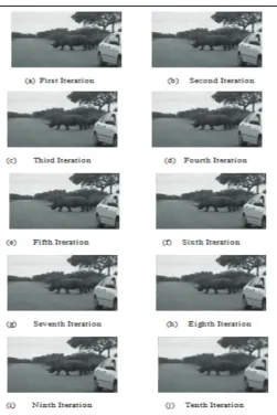
Fig. 6 shows how the true frame is constructed to low resolution frame. By using the interpolation techniques, the changes in the frame are low and medium for nearest neighborhood, bilinear method and Bayesian Super Resolution respectively. For 10 iterations, the frames can be resolved as super-resolution frame.
is decreasing. This indicates that the quality of image is improving.
With the increase in number of iterations, the reconstruction will
be very good and automatically the frame quality will increase.
Fig. 6: Results of Interpolation and Proposed Algorithms
Fig. 7: Result of Bayesian Algorithm with iteration as 10
The below given plots are the actual graphs obtained while MATLAB processing. Fig. 8 shows the PSNR plot for Nearest
Neighborhood (NN) (Red in color), Bilinear (BI) (Blue in color)
and Bayesian Super Resolution Algorithm (BSR) (Green in color). The plot shows that the PSNR value of proposed method is the highest among the other two methods. This indicates the quality of video of proposed method is relatively good than the nearest neighbourhood method and bilinear method. The maximum value is 32.80dB.
Fig. 9 shows the SSIM plot for Nearest Neighbourhood (Red in
color), Bilinear (Blue in color) and Bayesian Super Resolution Algorithm (Green in color).
Fig. 8: Plot of PSNR for rhinos.avi
Fig. 9: Plot of SSIM for rhinos.avi
From the above discussions and from Table 1, we can conclude that Bayesian approach is giving reliable result than interpolation technique. The plus points of proposed methodology is Low Resolution system scan be used as it is.
The heavy tails of the distribution of high resolution image can be captured in better way. The edges of the reconstructed image can be preserved in better way and it easily improves the video quality.
Table 1: Analysis of all the Three Methods Sr.
No. Method PSNR SSIM Quality
1. NN LESS LESS LOW
2. BI MEDIUM MEDIUM MEDIUM
3. BSR HIGH HIGH GOOD
In future, there is an idea to develop a Bayesian approach to joint
super-resolution and fusion of video sequences acquired with different modalities.
VII. Acknowledgment
I am indeed thankful to my guide Dr. S.S. Agrawal for her able
guidance and assistance to complete this paper; otherwise it would
not have been accomplished. I extend my special thanks to Head of Department of Electronics & Telecommunication, Dr. S.K Shah who extended the preparatory steps of this paper-work. I am also thankful to the head & Principle of STES’S, Smt. Kashibai Navale College of Engineering, Dr. A.V.Deshpande for his valued support
and faith on me.
References
[1] J. Chen, J. Nunez-Yanez, A. Achim,“Bayesian video super
resolution with heavy –tailed models”, IEEE transactions
on circuits and systems for video technology, Vol. 24, No.
6, pp. 905–914, Jun. 2014.
[2] A. Achim, E. Kuruoglu,“Image denoising using bivariate
alpha stable distributions in the complex wavelet domain”,
IEEE Signal Process. Lett., Vol. 12, No. 1, pp. 17–20, Jan.
2005.
[3] C.R. Dance, E.E. Kuruoglu,“Estimation of the Parameters of Skewed alpha-Stable Distributions”, Apr 1999.
[4] J. Chen, J. Nunez-Yanez, A. Achim,“Video super-resolution
using generalized Gaussian Markov random fields”, IEEE Signal Process. Lett., Vol. 19, No. 2, pp. 63–66, Feb. 2012.
[5] R. Tsai, T. Huang,“Multiframe image restoration and
registration”, Adv. Comput. Vis. Image Process., Vol. 1, No. 2, pp. 317–339, 1984.
[6] H. Takeda, P. Milanfar, M. Protter, M. Elad,“Super-resolution without explicit subpixel motion estimation”, IEEE Trans. Image Process., Vol. 18, No. 9, pp. 1958–1975, Sep. 2009. [7] J. Portilla, V. Strela, M. J. Wainwright, E. P. Simoncelli,
“Image denoising using scale mixtures of Gaussian in the wavelet domain”, IEEE Trans. Image Process., Vol. 12, No.
11, pp. 1338–1351, Nov. 2003.
Sruthi Kurup has received B. E degree in Electronics and Telecommunication Engineering from Rajiv Gandhi College of Engineering and Research
from RTM Nagpur University in 2012
and currently pursuing her M.E degree in Electronics and Telecommunication
with specialization in Signal Processing
from Smt. Kashibai Navale College of Engineering, Vadgaon (bk), Pune in
Savitribai Phule Pune university.
Prof. Sujata Agrawal has received
her B.E. degree in Electronics and Telecommunication Engineering from YCCE, Nagpur. She has also completed M.E. Electronics degree from Government Engineering
College, Aurangabad. She has
submitted her Ph. D thesis to RTM
Nagpur University. She joined as
an Assistant Professor in E&TC, Smt. Kashibai Navale College of Engineering, Pune in 2002. She is having 20 years of teaching
experience. She has till now 2 national and 11 international journal publications in her credit. She has attended and presented 2 papers