Coding for Information Storage

(1)

Thesis by Zhiying Wang

In Partial Fulfillment of the Requirements for the Degree of

Doctor of Philosophy

California Institute of Technology Pasadena, California

2013

(2)

c

(3)

(4)

Acknowledgements

I would like to acknowledge my advisor Professor Jehoshua (Shuki) Bruck for his constant guidance and support, without which this work would never exist. He is the most wonderful mentor one could hope for. He taught me not only how to do research, but also how to be a hard-working and kind person.

Itzhak Tamo has been a great friend and collaborator, even though I always have problem pro-nouncing his name. To work with and learn from him is inspiring and fun, and I would like to thank him for his amazing ideas and great help.

I also would like to thank Professor Anxiao (Andrew) Jiang, whom I believe is the most diligent and efficient researcher. Countless new ideas flow from him as the waves flow from the ocean. But more importantly, he cares about his students and friends as if they were family.

I would like to thank Professor Alexandros G. Dimakis, who introduced me to the distributed storage problem. He has so much positive energy in work and life that everybody near him cannot avoid being caught up into it.

I also would like to thank my friends and colleagues from the Paradise Lab: Professor Yuval Cassuto, Robert Mateescu, Dan Wilhelm, Hongchao Zhou, Eyal En Gad, and Eitan Yaakobi. Only because of them has life in an unfamiliar city been filled with joy and excitement.

(5)

Abstract

Storage systems are widely used and have played a crucial rule in both consumer and industrial products, for example, personal computers, data centers, and embedded systems. However, such system suffers from issues of cost, restricted-lifetime, and reliability with the emergence of new systems and devices, such as distributed storage and flash memory, respectively. Information theory, on the other hand, provides fundamental bounds and solutions to fully utilize resources such as data density, information I/O and network bandwidth. This thesis bridges these two topics, and proposes to solve challenges in data storage using a variety of coding techniques, so that storage becomes faster, more affordable, and more reliable.

We consider the system level and study the integration of RAID schemes and distributed storage. Erasure-correcting codes are the basis of the ubiquitous RAID schemes for storage systems, where disks correspond to symbols in the code and are located in a (distributed) network. Specifically, RAID schemes are based on MDS (maximum distance separable) array codes that enable optimal storage and efficient encoding and decoding algorithms. Withrredundancy symbols an MDS code can sustainrerasures. For example, consider an MDS code that can correct two erasures. It is clear that when two symbols are erased, one needs to access and transmit all the remaining information to rebuild the erasures. However, an interesting and practical question is: What is the smallest fraction of information that one needs to access and transmit in order to correct a single erasure? In Part I we will show that the lower bound of1/2is achievable and that the result can be generalized to codes with arbitrary number of parities and optimal rebuilding.

(6)

(7)

List of Figures

1.1 Global data traffic . . . 2

1.2 Trend of SSD . . . 2

1.3 Trend of cloud storage . . . 3

1.4 Errors in distributed storage . . . 4

1.5 Rebuild in distributed storage . . . 4

1.6 Iterative programming . . . 5

1.7 Rank modulation . . . 6

3.1 Repair of a(4, 2)EVENODD code . . . 16

3.2 Repair of an EVENODD code with p=5 . . . 19

3.3 Recovery in STAR code . . . 25

4.1 Rebuilding of a(4, 2)MDS array code . . . 28

4.2 Permutations for a zigzag code . . . 29

4.3 Generate the permutation . . . 30

4.4 A(5, 3)MDS array code . . . 32

4.5 Comparison among different code constructions . . . 46

4.6 Duplication code . . . 50

4.7 The induced subgraph ofD4 . . . 52

4.8 A(6, 3)MDS array code . . . 63

5.1 An MDS array code with two systematic and two parity nodes . . . 74

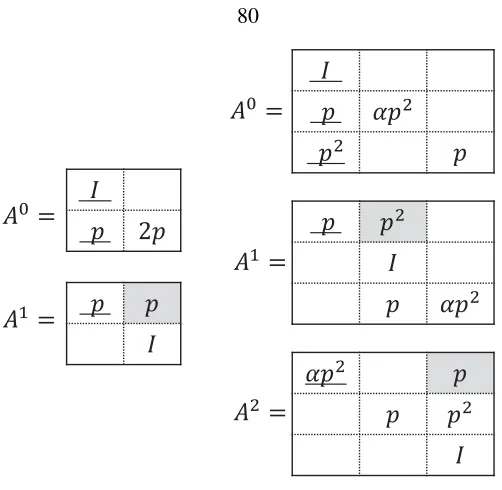
5.2 Parity matrices . . . 80

5.3 Rebuilding of a(4, 2)MDS array code . . . 81

6.1 (5, 3)zigzag code . . . 95

(11)

7.1 (n=6,k=4,l=2)code . . . 112

7.2 (n=8,k=6,l=4)code . . . 117

7.3 Vectors for(n=7,k=4,l=9)code . . . 125

7.4 (n=11,k=8,l=9)code . . . 125

8.1 A flash memory cell . . . 136

9.1 Labeled graphs forCI . . . 144

9.2 Capacity forC_I . . . 146

9.3 Labeled graphs forC(n, 2, 4, 1) . . . 148

9.4 Capacity forC . . . 149

9.5 Encoder and decoder for BRM . . . 149

9.6 Rate3 : 4finite-state encoder . . . 151

10.1 Directed graphs withn=3,k=1. . . 165

10.2 A cycle for 2-partial permutations out of 4 . . . 167

10.3 Insertion . . . 169

10.4 An insertion tree . . . 171

10.5 A generating tree of6out of3 . . . 173

10.6 Comparison of universal cycle algorithms . . . 181

11.1 Permutations of length 3 . . . 186

11.2 Encoder and decoder of a 1-error-correcting code . . . 190

11.3 2-error-correction rank modulation codes . . . 194

11.4 3-error-correction rank modulation codes . . . 195

11.5 The underlined binary code . . . 196

(12)

Chapter 1

Introduction

Information theory studies the compression, the storage, and the communication of information. Among these topics, the storage of data has attracted a large amount of interest among both in-dustrial and academic researchers in the era of information explosion, especially with the rapid development of the Internet. Moreover, the implementation of distributed storage and the success of new storage devices, such as flash memory, also provide people with new media for more data storage. Therefore, two of the most exciting topics in information theory today are information representation in distributed storage and flash memory, which will also be the two subjects of this thesis.

Network solution providers such as Cisco predicted that the amount of Internet data traffic will increase by32%every year from 2011 to 2016 [Cis12] (see Figure 1.1). And the overall data will reach45000petabytes per month next year (year 2014). This also indicates the huge demands for data storage in the near future. Therefore, it is an urgent challenge to invent reliable, inexpensive, high-performance and power-efficient information storage.

(13)

Figure 1.1: The amount of data traffic in the recent years. The compound average growth rate (CAGR) is32%every year. Source: Cisco [Cis12].

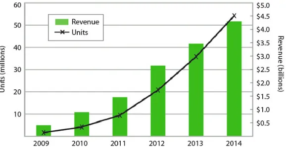
Figure 1.2: The trend of SSD in terms of unit and revenue. Source: SanDisk [Ore11].

the trend of SSD (solid state drive) in terms of unit and revenue estimated by SanDisk [Ore11]. Projections show that the number of SSD units will jump to 50 million by 2014.

(14)

Figure 1.3: The development of cloud storage in terms of number of subscribers. Source: Seagate [Woj12].

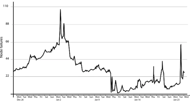
In distributed storage, as the system scales failures are inevitable. Hence redundant data must be stored in order to combat errors. Erasure correction codes are the most commonly used technique for this purpose. When a failure happens and repair is executed, a large data traffic in the network as well as large data I/O in each storage unit is generated. In fact, [SAP+13] shows that in a system with 3000 servers (or nodes) of Facebook, it is quite typical to have 20 or more node failures per day that triggers repair jobs (Figure 1.4). Moreover, with the current configuration the repair traffic is estimated around 10 to 20 percent of the total average of 2 petabytes per day cluster network traffic. Therefore, it is crucial to study practical solutions that repair with low traffic cost. Meanwhile, these challenges in distributed storage can be similar to those in a single data center. In such cases, our work can apply to both scenarios.

In Part I we study the rebuilding of distributed storage first proposed by [DGW+10]. Figure 1.5 shows an example of an erasure correction code called EVENODD [BBBM95] with four nodes. One can easily verify the following properties of this code. (i)Node size: each node has size two. (ii)Reconstruction: if we lose any two nodes the information bits a,b,c,d can be still computed from the rest nodes or 4 bits. (iii)Rebuilding: if only one node fails, transmitting only 3 bits we are able to solve the lost bits. Sometimes we can access or read some bits and directly transmit them such as Figure 1.5 (a). In other cases we need to access and compute before we transmit, such as bit

(15)

Figure 1.4: Number of failed nodes in a month in a distributed storage with 3000 nodes of Facebook [SAP+13].

(16)

Figure 1.6: Iterative programming towards different targets (dashed lines). The circles in the solid lines shows the result after each iteration [BSH05].

suffers from limited life time (105 write/erase cycles), read/write disturbances, limited retention, and high cost of erasure. For example, due to the high cost of erasure, decrease a data value is very expensive. As a result, the writing of data is processed in a very conservative interactive method in current flash technology. Figure 1.6 is from [BSH05] and shows that the average number of pulses required to hit a target in this example is 7 to 8. Here the current target corresponds to the desired value to store. One can see that writing can be very slow and thus degrades the performance of the system. For the consumer applications, these problems of flash are not critical because the requirement for the performance are topically not very high. However, they have to be solved in order to satisfy the enterprise requirements such as frequent fast access, long lifespan, and high reliability.

(17)

Figure 1.7: Information representation schemes in flash memory. (a) Absolute-value representation. Every cell must fall in one of the two target levels. Cell 1 and 2, respectively, represent value 0 and 1. (b) Rank modulation of length 2. Every two cells constitute a permutation. If the first cell is lower than the second, the permutation is (1,2) and represents value 0; otherwise the permutation is (2,1) and represents value 1.

is very expensive, the other cells will be merely increased.

This thesis strives to provide easier, faster, and more reliable ways to store data with the help of coding techniques. The rest of the thesis is divided into two parts: coding for distributed storage and coding for flash memory.

The rebuilding access or transmission problem of distributed storage will be more thoroughly explained in Chapter 2. Our contributions are inventing efficient rebuilding algorithm for existing codes in Chapter 3, constructing optimal rebuilding codes, zigzag codes, and their extensions in Chapter 4 and 5, rebuilding multiple failures in Chapter 6, and studying the relationship of the number of nodes and the node size in Chapter 7.

Chapter 8 gives a more detailed introduction to rank modulation in flash memory. We will study rank modulation with more constraints on the permutation size, e.g., bounded rank modulation in Chapter 9 and partial rank modulation in Chapter 10. Error correction in rank modulation will be discussed in Chapter 11.

(18)

Part I

(19)

Chapter 2

Introduction to the Rebuilding Problem

Distributed storage systems involving storage nodes connected over networks have become one of the most popular architecture in current file systems. MDS (maximum distance separable) codes can be used for erasure protection in distributed storage systems where encoded information is stored in a distributed manner. A code withrparity (redundancy) nodes is MDS if and only if it can recover from anyrerasures. For example, Reed-Solomon codes [RS60] are the most commonly seen MDS codes.

Moreover, a more general framework of file storage can be a collection of storage nodes located in a distributed or a centralized manner. RAID (redundant array of independent disks) is such a storage technique and it combines multiple disk drive components into a logical unit. MDS array codes are used extensively as the basis for RAID storage systems. An array code consists of a 2-D array where each column can be considered as a disk. We will use the term column, node, or disk interchangeably. We call the entries in the array symbols, elements, or blocks. Examples of MDS array codes are EVENODD [BBBM95, BBV96], B-code [XBBW99], X-code [XB99], RDP [CEG+04], and STAR-code [HX08].

If no more than r storage nodes are lost, then all the information can still be recovered from the surviving nodes. In order to correct r erasures, it is obvious that one has to access (or read) and transmit the information in all the surviving nodes. However, in practice it is more likely to encounter a single erasure rather thanrerasures. Suppose one node is erased, and instead of retriev-ing the entire file, if we are only interested in repairretriev-ing the lost node, then what is smallest amount of transmission or access needed? The amount of transmission is called therepair bandwidthand the amount of access if called rebuilding access. Assume a file of sizeM is stored in n nodes, each storing a piece of size M/k. Further assume we have access to d of the surviving nodes,

(20)

repair bandwidth of one node erasure was derived:

Md

k(d−k+1). (2.1)

Besides bandwidth and access, there are quite a few other key features of an array code in storage. We list some of them below, and in the following chapters we will study in more details on them for code constructions.

Systematic. A code is systematic if the information is stored exclusively in the firstknodes (sys-tematic nodes), and the redundancies are stored exclusively in the lastrnodes (parity nodes). The advantage of such codes is that information can be easily obtained from only the firstk

nodes.

Finite-Field Size It is the size of the finite field where all entries or symbols in the array belong to. One reason of the popularity of array code is its small field size and hence low computational complexity.

Update. It is the number of symbol rewrites when an information symbol is updated. It also equals the number of appearances of a symbol in the array code. If the code is MDS, any information symbol appears at leastr+1times, because otherwise we can erase those nodes containing this symbol and violate the MDS property. If each information symbol appears onlyr+1 times, we say the code isoptimal update.

Bandwidth. It is the smallest amount of data transmission for rebuilding a node erasure. If a code matches the bound (2.1) we say it isoptimal bandwidth. When the file size and the number of nodes is large, rebuilding is a common operation and takes up a large portion of network resources. Small bandwidth indicates low traffic consumption in the rebuilding process and is desirable for large systems.

Access. It is the smallest amount of data access for rebuilding a node erasure. Note that a transmit-ted symbol can be a function of many accessed symbols. As a result, the rebuilding access is always no less than the repair bandwidth. If the access of a code matches the bound (2.1) we say is itoptimal access. Small access leads to small disk I/O and also fast information retrieval.

(21)

nodesk. In order to achieve optimal rebuilding, sometimes each node needs to be subpack-etized into many symbols. The length of each column equals to the number of subpackets, denoted byl. We would like to havelsmall for givenkso that the file size can be flexible and the code can be easy to work with.

The problem of rebuilding or regenerating information in (distributed) storage systems has at-tracted considerable interest in recent years. A recent survey of the repair problem can be found in [DRWS11]. If we repair the lost information functionally, namely to obtain a function of the file and maintain the MDS property, [WDR07, Wu09] showed existence of codes using network coding techniques. If we repair the lost information exactly, [SR10b, CJM10] proved that the lower bound is asymptotically achievable when the column length l goes to infinity. However, the proofs in the above work are theoretical and is based on very large finite fields. Hence, it does not provide the basis for constructing practical codes with small finite fields. In [WD09] [CDH09], this lower bound is matched for exact repair by code constructions for k = 2, 3, or

n−1. In [RSKR09, SR10a, SRKR10] codes achieving the repair bandwidth lower bound were studied where the number of systematic nodes is less than the number of parity nodes (low code rate). And [CHL11, CJ11, CHLM11, PDC11b, PDC11a, TWB11, WTB11, TWB13] studied codes with more systematic nodes than parity nodes (high code rate) and finitel, and achieved the lower bound of the repair bandwidth.

In this thesis, we mainly focus on the regime of high-rate codes. We first try to rebuild erasures in existing erasure-correcting codes, and observe the advantages and disadvantages of such codes. Then we try to construct our own codes, which match the repair bandwidth/access lower bound and are therefore optimal.

In Chapter 3, we study the rebuilding of existing MDS array codes, such as EVENODD. Such codes are not only MDS but also binary codes, namely they only require XOR operations for en-coding and deen-coding. We show that when there are two redundancy nodes, to rebuild one erased systematic node, only3/4of the information needs to be transmitted. Interestingly, in many cases, the required disk I/O is also minimized.

Actually (2.1) shows that the lower bound of rebuilding access is a fraction of1/2. There is a gap between the lower bound and the existing array codes. In Chapter 4 we constructzigzag codes

(22)

MDS array codes that has optimal rebuilding access fraction of 1_r in the case of a single systematic erasure. Our array codes have efficient encoding and decoding algorithms (for the casesr= 2and

r =3they use a finite field of size3and4, respectively) and an optimal update property.

However, we have not yet solved the problem entirely. For a parity node erasure, all the in-formation needs to be accessed. Namely, constructing array codes with optimal rebuilding for an arbitrary erasure was left as an open problem. In Chapter 5, we solve this open problem and present array codes that achieve the lower bound (2.1) for rebuilding any single systematic or parity node.

We discuss other decoding problems in Chapter 6. For zigzag codes with two parities, we study how to correct one erasure, two erasures, or one column error. Notice that a column is composed of

lsymbols, we also discuss rebuilding an erased column in the presence of symbol errors. Moreover, we show that zigzag codes have optimal rebuilding for multiple erasures. Whenenodes are erased, we show that onlye/rfraction of the file needs to be accessed, for all1≤e≤r.

(23)

Chapter 3

Rebuild for Existing Array Codes

3.1 Introduction

Coding techniques for storage systems have been used widely to protect data against errors or era-sure for CDs, DVDs, Blu-ray Discs, and SSDs. Assume the data in a storage system is divided into packets of equal sizes. An (n,k)block code takes k information packets and encodes them into a total of npackets of the same size. Among coding schemes, maximum distance separable (MDS) codes offer maximal reliability for a given redundancy: anykpackets are sufficient to re-trieve all the information. Reed-Solomon codes [RS60] are the most well-known MDS codes that are used widely in storage and communication applications. Another class of MDS codes are MDS array codes, for example, EVENODD [BBBM95] and its extension [BBV96], B-code [XBBW99], X-code [XB99], RDP [CEG+04], and STAR code [HX08]. In an array code, each of the packets consists of a column of elements (one or more binary bits), and the parities are computed by XOR-ing some information bits. These codes have the advantage of low computational complexity over RS codes because the encoding and decoding only involve XOR operations.

(24)

recovery of single or double disk recovery for EVENODD, X-code, STAR, and RDP code.

In practice, there is a difference between erasures of the information (also called systematic) and the parity nodes. An erasure of the former will affect the information access time since part of the raw information is missing, however erasure of the latter does not have such an effect, since the entire information is still accessible. Moreover, in most storage systems the number of parity nodes is quite small compared to the number of systematic nodes. Therefore, our study focus on rebuilding for the systematic nodes. The rebuilding of a parity node will require transmitting all the information in the systematic nodes.

In the general framework of [DGW+10], an acceptable rebuilding is one that retains the MDS property and not necessarily rebuilds the original erased node, whereas, we restrict our solutions toexact rebuilding. Exact rebuilding has the benefit that we can retrieve the original information immediately if the code issystematic, i.e., the information are stored inknodes.

Moreover, we assume that all the surviving nodes are accessible. This is reasonable if the nodes are located in a single disk array, or if all the links in the storage network is available. By accessing more nodes, we can parallelize the rebuilding process, and read and transmit less information in total. However, for some cloud storage applications, the main repair performance bottleneck is the disk I/O overhead, which is proportional to the number of nodes involved in the repair process of a failed node. Therefore, codes with low number of accessed nodes, or locally repairable codes, are studied in the literature (e.g., [GHSY12] [OD11] [SRKV13] [TPD13]).

If the whole data object stored has sizeMbits, repairing a single erasure naively would require communicating (and reading) M bits from surviving storage nodes. Here we show that a single failed systematic node can be rebuilt after communicating only 3₄M+O(M1/2₎_{bits. Note that}

the cut-set lower bound [DGW+10] scales like 1₂M+O(M1/2_{), so it remains open if the repair}

communication for EVENODD codes can be further reduced. This question will be answered posi-tively in the next few chapters. Interestingly our repair scheme also requires significantly less disk I/O reads compared to naively reading the whole data object.

(25)

3.2 Definitions

AnR×narray code containsRrows andncolumns (or packets). Each element in the array can be a single bit or a block of bits. We are going to call an element ablock. In an(n,k)array code,

k information columns, or systematic columns, are encoded inton columns. Thetotal amount of informationisM= Rkblocks.

An EVENODD code [BBBM95] is a binary MDS array code that can correct up to 2 column erasures. For a prime number p ≥ 3, the code containsR = p−1rows andn = p+2columns, where the firstk = pcolumns are information and the last two are parity. And the information is

M = (p−1)pblocks.

We will write an EVENODD code as:

a1,1 a1,2 . . . a1,p b1,0 b1,1 a2,1 a2,2 . . . a2,p b2,0 b2,1

..

. ... ... ... ...

ap−1,1 ap−1,2 . . . ap−1,p bp−1,0 bp−1,1

And we define an imaginary rowap,j =0, for allj =1, 2, . . . ,p, where0is a block of zeros. The

slope 0orhorizontal parityis defined as

bi,0 =

p

∑

j=1

ai,j (3.1)

fori=1, . . . ,p−1. The addition here is bit-by-bit XOR for two blocks. A parity block ofslopev,

−p<v< pandv6=0is defined as

bi,v = p

∑

j=1

a_j_,<i+v(1−j)>+Sv= p

∑

j=1

a<i+v(1−j)>,j+Sv (3.2)

whereSv= ap,1+ap−v,2+· · ·+a<p+v>,p =∑_jp=1a<v(1−j)>,j and<x >= (x−1)mod p+1. Sometimes we omit the “<>” notation. Whenv =1, we call it theslope 1, ordiagonal parity. In EVENODD, parity columns are of slopes 0 and 1.

(26)

slope -1 and 1, and are placed as two additional rows, instead of two parity columns.

The code in [BBV96] extended EVENODD to more than 2 columns of parity. This code has

n = p+r,k = p, andR = p−1. The information columns are the same as EVENODD, butr

parity columns of slopes0, 1, . . . ,r−1are used. It is shown in [BBV96] that such a code is MDS whenr≤3and conditions for a code to be MDS are derived forr≤8.

STAR code [HX08] is an MDS array code withk = p,R = p−1,n = p+3, and the parity columns are of slope 0, 1, and -1.

Aparity groupBi,vof slopevcontains a parity blockbi,vand the information blocks in the sum in equations (3.1) (3.2), i = 1, 2, . . . ,p−1. Sv is considered as a single information block. If

v=0, it is ahorizontal parity group, and ifv =1, we call it adiagonal parity group.

By (3.1), each horizontal parity groupBi,0containsai,<k+1−i>∈Bk,1, for allk=1, 2, . . . ,p−

1. So we say Bi,0 crosses withBk,1, for allk = 1, 2, . . . ,p−1. Conversely, each diagonal parity

groupBi,1containsak,<i+1−k>∈Bk,0, for allk =1, 2, . . . ,p−1. Therefore,Bi,1crosses withBk,0

for allk=1, 2, . . . ,p−1. The shared block of two parity groups is called thecrossing. Generally, two parity groupsBi,vandBk,ucross, for v6= u,1 ≤i,k ≤ p−1. If they cross atap,<i+v> = 0,

we call it azero crossing. A zero crossing does not really exist since the p-th row is imaginary. A zero crossing occurs if and only if

u,v6=0and <i+v>=< k+u > (3.3)

Moreover, each information block belongs to only one parity group of slopev.

In this chapter, we use MDS array codes as distributed storage codes. We will give repair methods and compute the corresponding bandwidthγ.

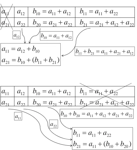
Example 3.1 Consider the EVENODD code with p = 3. Set a1,3 = a2,3 = 0 for all codewords, then the code will contain only 2 columns of information. The resulting code is a (4, 2) MDS code and this is calledshortenedEVENODD (see Figure3.1). It can be verified that if any node is erased, then sending 1 block from each of the other nodes is sufficient to recover it. And this actually

matches the bound (2.1). Figure3.1shows how to recover the first or the fourth column. Notice that a sum block is sent in some cases. For instance, to recover the first column, the sumb1,1+b2,1is sent from the fourth column.

(27)

22 12 21 21 22 21 20 22 21 22 11 11 12 11 10 12 11

a

b

a

b

a

b

a

b

a

12 21 11 21

11 b a a a

b

12

a

10 12

11

a

b

a

12 11

10 a a

b 12 21 11 21 11

)

(

₁₁ ₂₁

10

21

b

a

22 11 11 12 11 10 12 11

a

b

a

b

a

b

a

b

a

22 12 21 21 22 21 20 22

21

a

b

a

b

a

22 21 12 11 20

10 b a a a a

b 11 a 22 a

)

(

₁₀ ₂₀

11 21 22 11 11

b

a

b

a

b

Figure 3.1: Repair of a(4, 2)EVENODD code if the first column (top graph) or the fourth column (bottom graph) is erased. In both cases, three blocks are transmitted.

of data except the sum∑_ip₌−₁1bi,vfrom the parity node of slopev, for allvdefined in an array code. In addition, we assume that each node can transmit a different number of blocks.

3.3 Repair for Codes with Two Parity Nodes

First, let us consider the repair problem of losing one systematic node,n−d= 1, andn−k = 2. We will use EVENODD to explain the repair method, and the recovery will be very similar if RDP or X-code is considered.

By the symmetry of the code, we assume that the first column is missing. Each block in the first column must be recovered through either the horizontal or the diagonal parity group including this block. Suppose we usexhorizontal parity groups andp−1−xdiagonal parity groups to recover the column,0≤ x≤ p−1. These parity groups include all blocks of the first column exactly once.

Notice thatS1 =∑p

−1

i=1 bi,0+∑p

−1

i=1 bi,1, so we can send∑p

−1

i=1 bi,0from the(p+1)-th node, and

∑ip=−11bi,1from the(p+2)-th node, and recoverS1with 2 blocks of transmission. For the discussion

below, assumeS1is known.

(28)

1, 2, . . . ,i−1,i+1, . . . ,p−1, which isp−1blocks in total.

If two parity groups cross at one block, there is no need to send this block twice. As shown in Section 3.2, any horizontal and any diagonal parity group cross at a block, and each block can be the crossing of two groups at most once. There are x(p−1−x)crossings. The total number of blocks sent is

γ= xp

|{z}

horizontal

+ (p−1−x)(p−1)

| {z }

diagonal

+ 2 |{z}

S1

−x(p−1−x) | {z }

crossings

= (p−1)p+2−(x+1)(p−1−x) (3.4)

≥(p−1)p+2−(p2−1)/4= (3p2−4p+9)/4

The equality holds whenx= (p−1)/2orx= (p−3)/2, wherexis an integer.

This result states that we only need to send about3/4of the total amount of information. And the slopes of the nchosen parity groups do not matter as long as half are horizontal and half are diagonal. Moreover, similar repair bandwidth can be achieved using RDP or X-code. For RDP code, the repair bandwidth is

3(p−1)2 4

which was also derived independently in [XXLC10]. For X-code, the repair bandwidth is at most 3p2−2p+5

4

The derivation for RDP is the following. For RDP code, the firstp−1columns are information. The p-th column is the horizontal parity. The (p+1)-th column is the slope 1 diagonal parity (including the p-th column). The diagonal starting at ap,1 = 0 is not included in any diagonal

parities. Suppose the first column is erased. Each horizontal or diagonal parity group will require

p−1 blocks of transmission. Every horizontal parity group crosses with every diagonal parity group. Suppose (p−1)/2 horizontal parity groups and (p−1)/2 diagonal parity groups are transmitted. Then the total transmission is

γ= (p−1)(p−1)

| {z } p−1parity groups

− p−1

2

p−1 2 | {z }

crossings

= 3(p−1)

2

4

(29)

The derivation for X-code is as follows. For X-code, the (p−1)-th row is the parity of slope -1, excluding thep-th row. And the p-th row is the parity of slope 1, excluding the(p−1)-th row. Suppose the first column is erased. First notice that for each parity group, p−2 blocks need to be transmitted. To recover the parity block ap−1,1, one has to transmit the slope -1 parity group

starting at ap−1,1. To recover the parity block ap,1, the slope 1 parity group starting at ap,1 must

be transmitted. But it should be noted that by the construction of X-code, this slope 1 parity group essentially is the diagonal starting atap−1,1, except for the first elementap,1. Zero crossings happen

between two parity groups of slopes -1 and 1, starting atai,1andaj,1, if

<i+j>= p−2or < i+j>= p

Each slope 1 parity group has no more than 2 zero crossings with the slope -1 parity groups. Suppose we choose arbitrarily (p−1)/2slope 1 parity groups and(p−3)/2slope -1 parity groups for the information blocks in the first column. Then not considering the parity group con-tainingap,1, the number of slope 1 and slope -1 parity groups are both(p−1)/2. Excluding zero

crossings, each slope 1 parity group crosses with at least

(p−1)/2−2= (p−5)/2

slope -1 parity groups. The total transmission is

γ≤ p(p−2)

| {z } pparity groups

− p−1

2

p−5 2 | {z }

crossings

= 3p

2₋₂_p₊₅

4

Also, equation (3.4) is optimal in some conditions:

Theorem 3.2 The transmission bandwidth in (3.4) is optimal to recover a systematic node for EVENODD if no linear combinations are sent except∑_ip₌−₁1b_i_,_v, forv=0, 1.

Proof: To recover a systematic node, say, the first node, parity blocksbi,v,i=1, 2, . . . ,p−1 must be sent, wherev can be 0 or 1 for eachi. This is because ai,1is only included inbi,0orbi,1.

(30)

11 10 15 14 13 12

11

a

b

a

SystematicNodes ParityNodes

31 30 35 34 33 32 31 21 20 25 24 23 22 21 11 10 15 14 13 12 11

b

a

b

a

41 40 45 44 43 42

41

a

b

a

Figure 3.2: Repair of an EVENODD code withp =5. The first column is erased, shown in the box. 14 blocks are transmitted, shown by the blocks on the horizontal or diagonal lines. Each line (with wrap around) is a parity group. 2 blocks in summation form, ∑p_i₌−₁1bi,0,∑_ip=−11bi,1are also needed

but are not shown in the graph. The lower bound by (2.1) is

Md

(d−k+1)k =

M(n−1) (n−k)k =

p(p−1)(p+1)

2p =

p2−1 2

whered = n−1,n = p+2,k = p, andM = p(p−1). It should be noted that (2.1) assumes that each node sends the same number of blocks, but our method does not.

Example 3.3 Consider the EVENODD code with p = 5 in Figure 3.2. For 1 ≤ i ≤ 4, the code has information blocks ai,j, 1 ≤ j ≤ 5, and parity blocks bi,v, v = 0, 1. Suppose the first

column is lost. Then by (3.4), we can choose parity groupsB1,0,B2,0,B3,1,B4,1. The blocks sent are:

∑ip=−11bi,0,∑p

−1

i=1 bi,1,b1,0,b2,0,b3,1,b4,1 from the parity nodes and a1,2,a1,3,a1,4,a1,5,a2,2,a2,3,a2,4, a2,5,a4,5,a3,2 from the systematic nodes. Altogether, we send 16 blocks, the number specified by

(3.4). We can see thata1,3is the crossing ofB1,0andB3,1. Similarly,a1,4,a2,2,a2,3are crossings and are only sent once for two parity groups.

3.4 r

Parity Nodes and One Erased Node

Next we discuss the repair of array codes withr columns of parity,r ≥ 3. And we consider the recovery in case of one missing systematic column. In this section, we are going to use the extended EVENODD code [BBV96], i.e., codes with parity columns of slope0, 1, . . . ,r−1. Similar results can be derived for STAR code. Suppose the first column is erased without loss of generality.

(31)

Notice that0 ≤ n ≤ A and each slope has no more than d(p−1)/3e but no less thanb(p−

1)/3c= Aparity groups.

Since there are three different slopes, there are crossings between slope 0 and 1, slope 1 and 2, and slope 2 and 0. For any two parity groupsBi,1andBk,2,< k−i>6= 1, so (3.3) does not hold.

Hence no zero crossing exists for the chosen parity groups. Hence, every crossing corresponds to one block of saving in transmission. However, the total number of crossings is not equal to the sum of crossings between every two parity groups with different slopes. Three parity groups with slopes 0, 1, and 2 may share a common block, which should be subtracted from the sum.

Notice that the parity groupBi,vcontains blockai−vy,y+1. The modulo function “<>” is omitted

in the subscripts. For three transmitted parity groups B3n,0,B3m+1,1,B3l+2,2, if there is a common

block in columny+1, then it is in row3n≡3m+1−y≡3l+2−2y (mod p). To solve this, we gety≡ 3(m−n) +1≡ 3(l−m) +1 (mod p), orm−n≡ l−m (modp). Notice0 ≤

n,m,l < p/3, so−p/3 < m−n,l−m < p/3. Therefore,m−n = l−mwithout modulo p. Thusl−nmust be an even number. For fixedn, eithern≤m≤l≤ A, and there are no more than (A−n)/2+1solutions for(m,l); or0 ≤ l< m< n, and the number of(m,l)is no more than

n/2. Hence, the number of(n,m,l)is no more than∑_nA₌₁((A−n)/2+1+n/2) = A2/2+A. The total number of blocks in the p−1chosen parity groups is less thanp(p−1). There are no less than Aparity groups of slopev, for all0 ≤ v ≤ 2, therefore for0 ≤ u < v ≤ 2, parity groups with slopesuandvhave no less thanA2 crossings. Hence the total number of blocks sent in order to recover one column is:

γ < p(p−1)

| {z } p−1parity groups

−

3 2

A2

| {z }

crossings

+ A

2₊₂_A

2 | {z }

common

+ 3 |{z}

∑ip=−11bi,v

< 13 18p

2₊ 17

9 p− 47

18 (3.5)

where(p−4)/3 < A ≤ (p−1)/3. The above estimation is an upper bound because there may be better ways to assign the slopes of each parity group. Whenr =3, we need to send no more than about13M/18blocks.

By abuse of notation, we write Bm,v = {a<m+v(1−j)>,j : j = 2, . . . ,p} as the set of blocks (including the imaginaryp-th row) in the parity group exceptSvandam,1. LetMv ⊆ {1, 2, . . . ,q}, 0≤ v ≤r−1, be disjoint sets such that∪r−1

v=0Mv = {1, 2, . . . ,q−1}. LetBMv,v = ∪m∈MvBm,v.

(32)

m1)/(v2−v1) ≡ (m3−m2)/(v3−v2) ≡ . . .(mk−mk−1)/(vk−vk−1)modp}|, for k ≥ 3,

and0≤v1 <v2 <· · ·< vk ≤r−1. Then we have the following theorem:

Theorem 3.4 For the extended EVENODD withr ≥ 3, the repair bandwidth for one erased sys-tematic node is

γ < p(p−1) +p+r−

∑

0≤v1<v2≤r−1

|Mv1||Mv2|

+

∑

0≤v1<v2<v3≤r−1

f(v1,v2,v3)− · · ·+ (−1)r−1f(0, 1, . . . ,r−1) (3.6)

Proof: Suppose the first column is missing and we transmit the parity groupsBm,v,m ∈ Mv forv = 0, 1, . . . ,r−1. Since the union ofMv covers{1, 2, . . . ,q−1}, all the blocks in the first column can be recovered. The repair bandwidth is the cardinality of the union of BMv,v plus the

number of zero crossings and the summation blocks∑_ip₌−₁1bi,v. The number of zero crossings is no more than the size of the imaginary row,p. The number of the summation blocks isr.

By inclusion–exclusion principle, the cardinality of the union ofBMv,vis

∑

0≤v≤r−1

|BMv,v| −

∑

0≤v1<v2≤r−1

|BMv₁,v1∩BMv₂,v2|

+

∑

0≤v1<v2<v3≤r−1

|BMv₁,v1∩BMv₂,v2∩BMv₃,v3| − · · ·+ (−1)

r−1_|_B

M0,0∩BM1,1. . .BMr−1,r−1|

Every |Bm,v| ≤ p, so∑0≤v≤r−1|BMv,v| ≤ p(p−1). Every two parity groups Bm1,v1,Bm2,v2

cross at a block. Hence |BMv₁,v1 ∩BMv₂,v2| = |Mv1||Mv2|. Since Bm,v contains a<m+v(1−j)>,j,

j=2, . . . ,p, the intersection of more than two parity groupsBm1,v1, . . . ,Bmk,vk is equivalent to the

solutions of

m1−v1y≡m2−v2y≡ · · · ≡mk−vkymodp wherey+1is the column index of the intersection. Or,

y≡ m2−m1

v2−v1

≡ · · · ≡ mk−mk−1

vk−vk−1

modp

Therefore,

|BMv₁,v1 ∩BMv₂,v2∩. . .BM_vk,vk|= f(v1,v2, . . . ,vk)

And (3.6) follows.

(33)

forv =0, 1, 2. Forr =4, 5, we can derive similar bounds by defining Mv. Choose

Mv ={rn+v: 1≤rn+v≤ p−1} (3.7)

forv= 0, 1, . . . ,r−1. LetA =b(p−1)/rc. And for0≤ v1 < v2 < v3 ≤r−1, f(v1,v2,v3)

becomes the number of(n1,n2,n3),1≤rni+vi ≤ p−1, such that

(n2−n1)(v3−v2)≡(n3−n2)(v2−v1)mod p

Since −p/r < n2−n1,n3−n2 < p/r, and (v3−v2) + (v2−v1) < r, the above equation

becomes

(n2−n1)(v3−v2) = (n3−n2)(v2−v1)

without modulop. Therefore,

n3−n1 = (n3−n2) + (n2−n1)

= c·lcm(v3−v2,v2−v1)

1

v3−v2

+ 1

v2−v1

= c v3−v1

gcd(v3−v2,v2−v1)

where c is an integer constant, lcm is the least common multiplier and gcd is the greatest com-mon divisor. And for fixed n1, the number of solutions for (n2,n3)is no more than 1+ (A− n1)gcd(v3−v2,v2−v1)/(v3−v1), whenn1 ≤ n2 ≤ n3 ≤ A; and no more thann1gcd(v3− v2,v2−v1)/(v3−v1), when0≤ n3< n2< n1. The number of(n1,n2,n3)is

f(v1,v2,v3) <

∑

n1

1+ (A−n1+n1)

gcd(v3−v2,v2−v1) v3−v1

= A

1+Agcd(v3−v2,v2−v1) v3−v1

Similarly, for four parity groups,

f(v1,v2,v3,v4)> A

1+ (A+2)gcd(v4−v3,v3−v2,v2−v1)

v4−v1

(34)

For five parity groups,

f(v1,v2,v3,v4,v5)< A+A2

gcd(v5−v4,v4−v3,v3−v2,v2−v1) v5−v1

Whenr=4, equation (3.6) becomes

γ< p(p−1) +p+4−

∑

0≤v1<v2≤3

|Mv1||Mv2|+

∑

0≤v1<v2<v3≤3

f(v1,v2,v3)− f(0, 1, 2, 3)

By the previous equations,

f(0, 1, 2),f(1, 2, 3)< A(1+A/2)

f(0, 1, 3),f(0, 2, 3)< A(1+A/3)

f(0, 1, 2, 3)> A(1+ (A+2)/3

And the repair bandwidth is

γ≈ p2−

4 2 (p 4)

2_{+ (}₂_×1

2+2× 1 3)(

p

4)

2₋ 1

3(

p

4)

2₌ 7

24p

2

where the terms of lower orders are omitted. Whenr=5, we can use (3.6) again and get

γ≈ p2+ (−

5 2 +4 2+ 4 3+ 2 4− 2 3− 3 4 + 1 4)( p 5)

2 ₌ 53

75p

2

where the terms of lower orders are omitted.

It should be noted that the number of common blocks affects the bandwidth a lot. If we consider only the first 4 terms in (3.6), any assignment ofMvwith equal sizes will result in a lower bound of

γ>(r+1)p2/(2r)≈ p2/2, whenris large. But due to the common blocks, the trueγvalues for

r =4, 5using (3.7) has only slight improvement compared to the case ofr=3.

(35)

3.5 Three Parity Nodes and Two Erased Nodes

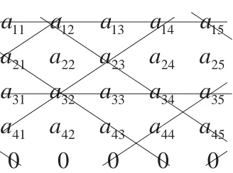
Up to now, we have considered the recovery problem given that one column is erased. Next, let us assume that two information columns are erased and we need to recover them successively. So we first recover one of the erased nodes, and then the other one. The first recovery is discussed in this section, and the second recovery was already discussed in the previous sections. Suppose we have 3 columns of parity with slopes -1, 0, and 1, which is in fact the STAR code in [HX08]. Again, the arguments can be applied to extended EVENODD in a similar way. Without loss of generality, assume the first and(x+1)-th columns are missing,1≤x ≤ p−1.

LetBi,0,Bi,1, andBi,−1bei-th parity group of slope 0, 1, and -1, respectively,i=1, 2, . . . ,p−1.

The following are3(p−1)/2parity groups that repair the first column: B0,−1,Bx,0,B2x,1,B2x,−1, B3x,0,B4x,1, . . . , B(p−3)x,−1,B(p−2)x,0,B(p−1)x,1. For each parity block above, the corresponding

recovered blocks are: ax,1+x,ax,1,a2x,1,a3x,1+x,a3x,1,a4x,1, . . . ,a(p−2)x,1+x,a(p−2)x,1,a(p−1)x,1. An

example ofp=5,x=1is shown in Figure 3.3.

Rearrange the columns in the following order: columns1, 1+x, 1+2x, . . . , 1+ (p−1)x (ev-ery index is computed modulo p). We can see that the chosen parity groups Bjx,0, j = x, 3x, . . . ,

(p−2)x contain the blocks in rows Z = {x, 3x, . . . ,(p−2)x}. Bjx,1 contains blocks ajx,1, a(j−1)x,1+x, . . . ,a(j−p+1)x,1+(p−1)x, for j = 2, 4, . . . ,p−1. And similarly Bjx,−1 contains blocks ajx,1,a(j+1)x,1+x, . . . ,a(j+p−1)x,1+(p−1)x, forj=0, 2, . . . ,p−3.

Now notice that the blocks included in the above parity groups have the (1+x)-th column as the vertical symmetry axis. That is, the row indices of the blocks needed in columns 1 and 1+2xare the same; those of columns1+ (p−1)xand1+3xare the same; ...; those of columns 1+ (p+3)x/2and1+ (p+1)x/2are the same. For example, the second column in Figure 3.3 is the symmetry axis. Thus, we only need to consider columns1+2x, 1+3x, . . . , 1+ (p+1)x/2.

For columns1+ix, whereiis even and2 ≤ i ≤ (p+1)/2, parity groups {B2x,1,B4x,1, . . . , B(p−1)x,1}include the blocks in rowsX= {2x, 4x, . . . ,(p−1−i)x}. And parity groups{B0,−1, B2x,−1, . . . ,B(p−3)x,−1}include the blocks in rowsY = {ix,(i+2)x, . . . ,(p−1)x}. Since2 ≤ i ≤ (p+1)/2, we have i ≤ (p−1−i) +2, and X∪Y = {2x, 4x, . . . ,(p−1)x}. Hence

X∪Y∪Z={1, 2, . . . ,p−1}. Thus every block in Column1+ixneeds to be sent, for eveni. Similarly, for columns 1+ix, whereiis odd and 3 ≤ i ≤ (p+1)/2, parity groups {B2x,1, B4x,1, . . . ,B(p−1)x,1}include the blocks in rowsX={(p−i+2)x,(p−i+4)x, . . . ,(p−1)x}.

(36)

15 14

13 12

11

a

35 34 33 32 31 25 24 23 22 21

a

0

45 44 43 42

41

a

Figure 3.3: The recovery strategy for the first column in STAR code when the first and second columns are missing. p=5,x=1.

3)x}. Since 2 ≤ i ≤ (p+1)/2, we havei−3 < p−i+2, and X∪Y = {2x, 4x, . . . ,(i−

3)x,(p−i+2)x,(p−i+4)x, . . . ,(p−1)x}. Therefore, the rows not included inXorYorZ

areW = {(i−1)x,(i+1)x, . . . ,(p−i)x}and|W|= (p+3)/2−i. The total saving in block transmissions for all the columns is:

2

∑

iodd,3≤i≤(p+1)/2

(p+3

2 −i) =  



(p−1)2

8 ,

p+1 2 odd

(p+1)(p−3)

8 ,

p+1 2 even

The above argument can be summarized in the following theorem.

Theorem 3.5 When two systematic nodes are erased in a STAR code, there exist a strategy that transmit about7/8of all the information blocks, and about1/2of all the parity blocks so as to recover one node.

The repair bandwidthγin the above theorem is about7p2/8. Comparing it to the lower bound

(2.1), _k₍_dM₋_kd₊₁₎ = p(p−1₂)(_pp+1) ≈ p₂2, we see a gap of 3₈p2 in total transmission.

3.6 Conclusions

(37)

simple and also requires smaller disk I/O to read data during repairs.

(38)

Chapter 4

Zigzag Code

4.1 Introduction

With r redundancy symbols, an MDS code is able to reconstruct the original information if no more thanr symbols are erased. An array code is a two-dimensional array, where each column corresponds to a symbol in the code and is stored in a disk in the RAID scheme. We are going to refer to a disk/symbol as a node or a column interchangeably, and an entry in the array as an element.

In this chapter, we will study the rebuilding access instead of bandwidth. Suppose that some nodes are erased in a systematic MDS array code, we will rebuild them by accessing (reading) some information in the surviving nodes, all of which are assumed to be accessible. The fraction of the accessed information in the surviving nodes is called therebuilding ratio, or simplyratio. Ifrnodes are erased, then the rebuilding ratio is1since we need to read all the remaining information. Is it possible to lower this ratio for less thanrerasures? Apparently, it is possible. The ratio of rebuilding a single systematic node was shown to be3₄+o(1)for EVENODD as shown in the previous chapter. Figure 4.1 shows an example of our new MDS code with2 information nodes and2 redundancy nodes, where every node has2elements, and operations are over the finite field of size3. Consider the rebuilding of the first information node. It requires access to3elements out of6(a rebuilding ratio of 1₂), becausea = (a+b)−bandc= (c+b)−b.

It should be noted that the rebuilding ratio counts the amount of information accessed from the system. Therefore, if we can minimize the rebuilding ratio, then we also achieve optimal disk I/O, which is an important measurement in storage.

(39)

Encode to (4,2)

MDS array code

Information

b a r1

d c r2

d a z1 2

b c z2

b a

c

d d

c b a

b a r1

b c z2

b

Figure 4.1: Rebuilding of a (4, 2)MDS array code overF3. Assume the first node (column) is

erased.

over the network in order to rebuild the erased nodes. In contrast to our concept ofrebuilding ratioa transmitted element of data can be a function of a number of elements that are accessed in the same node. In addition, we restrict ourselves toexactrebuilding. It is clear that our framework is a special case of the general framework, hence, the repair bandwidth is a lower bound on the rebuilding ratio. Letnbe the total number of nodes andkbe the number of systematic nodes. Suppose a file of size

M is stored in an (n,k) MDS code, where each node stores an information of sizeM/k. The number of redundancy/parity nodes isr = n−k, and in the rebuilding process all the surviving nodes are assumed to be accessible. A lower bound on the repair bandwidth for an(n,k)MDS code was derived in [DGW+10]:

M

k ·

n−1

n−k.

It can be verified that Figure 4.1 matches this lower bound. Note that the above formula represents the amount of information, it should be normalized to reach the ratio. The normalized bandwidth compared to the size of the remaining array M(n_k−1) is

ratio= 1

n−k =

1

r. (4.1)

A number of researchers addressed the construction of optimal repair-bandwidth codes [Wu09, WD09, RSKR09, SR10a, SRKR10, SR10b, CJM10, WDR07, RSK11], however they all have low code rate, i.e.,k/n< 1/2. Moreover, related work on constructing codes with optimal rebuilding appeared independently in [CHL11, PDC11b]. Their constructions are similar to this work, but use larger finite-field size.

(40)

0 1 2 R Z

0 ♣ ♠ ♥ ♣

1 ♥ ♦ ♣ ♥

2 ♠ ♣ ♦ ♠

3 ♦ ♥ ♠ ♦

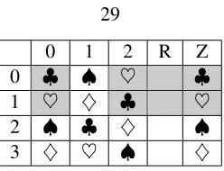
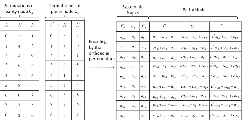
Figure 4.2: Permutations for zigzag sets in a (5, 3) code with 4rows. Columns 0, 1, and 2 are systematic nodes and columns R, and Z are parity nodes. Each element in column R is a linear combination of the systematic elements in the same row. Each element in column Z is a linear combination of the systematic elements with the same symbol. The shaded elements are accessed to rebuild column 1.

property, namely, when an information symbol which is an element from the field is rewritten, only the element itself and one element from each parity node needs an update. In total r+1 elements are updated. For an MDS code, this achieves the minimum reading/writing during writing of information. Hence, in the case of a code with2 parities only3 elements are updated. Under such assumptions, we will prove that every parity element is a linear combination of exactly one information element from each systematic column. We call this set of information elements aparity set. Moreover, the parity sets of a parity node form a partition of the information array.

For example, in Figure 4.1 the first parity node corresponds to parity sets{a,b},{c,d}, which are elements in rows. We say this node is therow parityand each row of information forms arow set. The second parity node corresponds to parity sets{a,d},{c,b}, which are elements in zigzag lines. We say that it is thezigzag parityand the parity set is called azigzag set. For another example, Figure 4.2 shows a code with3systematic nodes and2parity nodes. Row parityRis associated with row sets. Zigzag parityZ is associated with sets of information elements with the same symbol. For instance, the first element in columnRis a linear combination of the elements in the first row and in columns0, 1, and2. And the♣in column Z is a linear combination of all the♣elements in columns0, 1, and2. We can see that each systematic column corresponds to a permutation of the four symbols. For instance, if read from top to bottom, column0corresponds to the permutation [♣,♥,♠,♦]. In general, we will show that each parity relates to a set of a permutations of the

systematic columns. Without loss of generality, we assume that the first parity node corresponds to identity permutations, namely, it is linear combination of rows.

(41)

0 1 2

3

(0,0) (0,1) (1,0)

(1,1)

+(1,0) integer to

binary

binary to integer

2 3 0

1 (1,0)

(1,1) (0,0)

(0,1)

Figure 4.3: Generate the permutation by the binary vector(1, 0). Assumem=2.

If a single systematic node is erased, we will rebuild each element in the erased node either by its corresponding row parity or zigzag parity, referred to as rebuild by row (or by zigzag). In particular, we access the row (zigzag) parity element, and all the elements in this row (zigzag) set, except the erased element. For example, consider Figure 4.2, suppose that the column labeled1is erased, then one can access the8shaded elements and rebuild its first two elements by rows, and the rest by zigzags. Namely, only half of the remaining elements are accessed. It can be verified that for the code in Figure 4.2, all the three systematic columns can be rebuilt by accessing half of the remaining elements. Thus the rebuilding ratio is1/2, which is the lower bound expressed in (4.1).

The key idea in our construction is that for each erased node, the accessed row sets and the zigzag sets have a large intersection-resulting in a small number of accesses. Therefore it is cru-cial to find the permutations satisfying the above requirements. In this chapter, we will present an optimal solution to this question by constructing permutations that are derived from binary vec-tors. This construction provides an optimal rebuilding ratio of1/2for any erasure of a systematic node. To generate the permutation over a set of integers from a binary vector, we simply add to each integer the vector and use the sum as the image of this integer. Here each integer is ex-pressed as its binary expansion. For example, Figure 4.3 illustrates how to generate the permutation on integers {0, 1, 2, 3} from the binary vector v = (1, 0). We first express each integer in bi-nary: (0, 0),(0, 1),(1, 0),(1, 1). Then add (mod2) the vectorv = (1, 0)to each integer, and get (1, 0),(1, 1),(0, 0),(0, 1). At last change each binary expansion back to integer and define it as the

image of the permutation: 2, 3, 0, 1. Hence,0, 1, 2, 3 are mapped to 2, 3, 0, 1 in this permutation, respectively. This simple technique for generating permutations is the key in our construction. We can generalize our construction for arbitraryr(number of parity nodes) by generating permutations usingr-ary vectors. Our constructions are optimal in the sense that we can construct codes withr

parities and rebuilding ratio of1/r.

(42)

enough field size the code can be made MDS. In addition, a key result we prove is that for a code with two parity nodes, the field size is3, and this field size is optimal. Moreover, the field size is4 in the case of three parity nodes.

In addition, our codes have an optimalarray sizein the sense that for a given number of rows, we have the maximum number of columns among all systematic codes with optimal ratio and update. However, the length of the array is exponential in the width. We study different techniques for making the array wider, and the ratio will be asymptotically optimal when the number of rows increases. We mainly consider the case of two parities. One approach is to directly construct a larger number of permutations from binary vectors, and another is to use the same set of permutations multiple times.

In summary, the main contribution of this chapter is the first explicit construction of systematic (n,k)MDS array codes for any constantr = n−k, which achieves optimal rebuilding ratio of 1_r. Our codes have a number of useful properties:

• They are systematic codes, hence it is easy to retrieve information.

• They have high code ratek/n, which is commonly required in storage systems.

• They have optimal update given a finite filedFq, namely, when an information element is updated, onlyr+1elements in the array need update.

• The rebuilding of a failed node requires no computation in each of the surviving nodes, and thus achieves optimal disk I/O.

• The encoding and decoding of the codes can be easily implemented forr = 2, 3, since the codes use small finite fields of size 3 and 4, respectively.

• They have optimal array size (maximum number of columns) among all systematic, optimal-update, and optimal-ratio codes. Moreover, we also have asymptotically optimal codes that have better array size.

• They achieve optimal rebuilding ratio of 1_r when a single systematic erasure occurs.

(43)

0

f f1 f2

0 1 3 2 2 3 0 1 3 0 2

1 z0 a0,02a2,12a1,2

2 , 0 1 , 3 0 , 1

1 a 2a a

z 2 , 3 1 , 0 0 , 2

2 a a a

z 2 , 2 1 , 1 0 , 3

3 a a 2a

z 2 , 3 1 , 3 0 , 3

3 a a a

r 2 , 0 1 , 0 0 , 0

0 a a a

r 2 , 1 1 , 1 0 , 1

1 a a a

r 2 , 2 1 , 2 0 , 2

2 a a a

r

0

C C1 C2 C3 C4

0 , 0 a 0 , 1 a 0 , 2 a 0 , 3

a a3,1 a3,2 1 , 1

a a1,2 1 , 0

a a0,2

1 , 2

a a2,2

Encoding by the orthogonal permutations Orthogonal set of

permutations Systematic nodes Parity nodes

(a) (b)

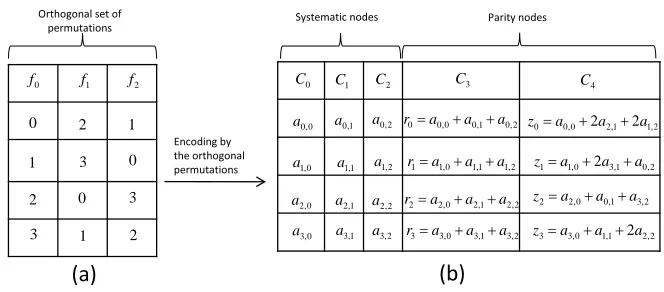
Figure 4.4:(a)The set of orthogonal permutations as in Theorem 4.3 with setsX0 ={0, 3},X1 =

{0, 1},X2 = {0, 2}. (b)A(5, 3)MDS array code generated by the orthogonal permutations. The

first parity columnC3is the row sum and the second parity columnC4is generated by the zigzags.

For example, zigzagz0contains the elementsai,j that satisfy fj(i) =0.

4.2 (

k

+

2,

k

)

MDS Array Code Constructions

Notations: In the rest of the chapter, we are going to use[i,j]to denote {i,i+1, . . . ,j}and [i] to denote {1, 2, . . . ,i}, for integers i ≤ j. And denote the complement of a subset X ⊆ M as

X = M\X. For a matrix A, AT denotes the transpose ofA. For a binary vectorv = (v1, ...,vn) we denote byv= (v1+1 mod 2, ...,vn+1 mod 2)its complement vector. The standard vector basis of dimensionmwill be denoted as{ei}mi=1and the zero vector will be denoted ase0.For two

binary vectorsv= (v1, . . . ,vm),u= (u1, . . . ,um), the inner product isv·u=∑mi=1viui mod 2. For two permutations f,g, denote their composition by f g.

In this section we give the construction of MDS array code with two parities and optimal re-building ratio1/2for one erasure, which uses a finite field of optimal size3.

4.2.1 Constructions

Let us define an MDS array code with 2 parities. Let A = (ai,j)be an information array of size

p×k over a finite field F, where i ∈ [0,p−1],j ∈ [0,k−1]. We add to the array two parity columns and obtain an(n = k+2,k)MDS code of array size p×n. Let the two parity columns be the row parity Ck = (r0,r1, ...,rp−1)T, and the zigzag parityCk+1 = (z0,z1...,zp−1)T. Let

{f0,f1, . . . ,fk−1} be zigzag permutations on [0,p−1] associated with the systematic columns

(44)

line: Z_l = {ai,j|fj(i) = l}. Then define the row parity element asrl = ∑a∈Rlαaaand the zigzag

parity element aszl = ∑a∈Zl βaa, for some sets of coefficients{αa},{βa} ⊆ F. We can see that

each parity element contains exactly one element from each systematic column, and we will show in Section 4.3 that this is equivalent to optimal update.

For example, in Figure 4.4 (a), we show three permutations on[0, 3]. Therefore we have the 0th zigzag setZ0 = {a0,0,a2,1,a1,2}. The 0th row set is by defaultR0 = {a0,0,a0,1,a0,2}. And in (b)

we show the corresponding code. ColumnsC0,C1,C2 are systematic columns. The row parityC3

sums up elements in a row, and each element in the zigzag parityC4is a linear combination of the

elements in some zigzag set. For instance,r0(orz0) is a linear combination of elements inR0(or Z0, respectively). Actually, this example is the code in Figure 4.2 with more details.

Therebuilding ratiois the average fraction of accessed elements in the surviving systematic and parity nodes while rebuilding one systematic node. A more specific definition will be given in the next section. In order to rebuild a systematic node, each erased element can be computed either by using its row set or by zigzag set. During the rebuilding process, an element is said to be rebuilt by row (zigzag), if we use the linear equation of its row (zigzag) set in order to compute its value. Solving this equation is done simply by accessing and reading in the surviving columns the values of the rest of the intermediates.

From the example in Figure 4.2, we know that in order to get low rebuilding ratio, we need to find zigzag sets{Zl}(and hence permutations {fi}) such that the row and zigzag sets used in the rebuilding intersect as much as possible. Moreover, it is clear that the choice of the coefficients is crucial if we want to ensure the MDS property. Noticing that all elements and all coefficients are from some finite field, we would like to choose the coefficients such that the finite-field size is as small as possible. So our construction of the code includes two steps:

1. Find zigzag permutations to minimize the ratio. 2. Assign the coefficients such that the code is MDS.

Next we generate zigzag permutations using binary vectors. We assume that the array has

p=2m_rows.

(45)

Let v ∈ _Fm

2 be a binary vector of length m. We define the permutation fv : [0, 2m−1] →

[0, 2m −1]by fv(x) = x+v, where x is represented in its binary representation. For example, whenm=2,v= (1, 0),x =3,

f(1,0)(3) =3+ (1, 0) = (1, 1) + (1, 0) = (0, 1) =1.

In other words, in order to get a permutation fromv, we first write all integers in[0, 2m−1]in binary expansion, then add vectorv, and at last convert binary vectors back to integers. This procedure is illustrated in Figure 4.3. Thus we can see that the permutation fv in vector notation is [2, 3, 0, 1]. One can check that this is actually a permutation for any binary vectorv. Next we present the code construction.

Construction 4.1 LetAbe the information array of size2m×k. LetT={v0,v1, . . . ,vk−1} ⊆Fm2 be a set of vectors of sizek. Forv∈T, we define the permutation fv :[0, 2m−1]→[0, 2m−1]by

fv(x) =x+v. Construct the two parities as row and zigzag parities.

For example, in Figure 4.4 (a), the three permutations are generated by vectorsv0= (0, 0),v1 =

(1, 0),v2= (0, 1). In Figure 4.4 (b), the code is constructed with the row and the zigzag parities.

4.2.2 Rebuilding Ratio

Let us present therebuilding algorithm:We define for a nonzero vectorv,Xv ={x∈ [0, 2m−1]:

x·v = 0}as the set of integers whose binary representation is orthogonal to v. For example,

X(1,0) = {0, 1}. Ifvis the zero vector we define Xv = {x ∈ Fm2 : x·(1, 1, ..., 1) =0}. For ease

of notation, denote the permutation fvj as fjand the setXvj asXj. Assume columnjis erased, and

defineSr = {ai,j : i∈ Xj}andSz = {ai,j : i ∈/ Xj}. Rebuild the elements inSrby rows and the elements inSzby zigzags.

Example 4.2 Consider the code in Figure4.4. Suppose node 1 (columnC1) is erased. SinceX1 = Xv1 = X(1,0) = {0, 1}, we will rebuild a0,1,a1,1 ∈ Sr by row parity elementsr0,r1, respectively.

(46)

the elementsa0,0,a0,2,a1,0,a1,2, and the following four parity elements

r0 =a0,0+a0,1+a0,2

r1 =a1,0+a1,1+a1,2

z_f₁(2) =z0=a0,0+2a2,1+2a1,2

z_f₁(3) =z1=a1,0+2a3,1+a0,2.

Here f1(2) = fv1(2) = f(1,0)(2) =0andzf1(2) =z0. Similarly, f1(3) = 1andzf1(3) =z1. Note

that each of the surviving node accesses exactly 1₂ of its elements. Similarly, if node 0 is erased, we

haveX0 = {0, 3}so we rebuild a0,0,a3,0 by row anda1,0,a2,0 by zigzag. Since X2 = {0, 2}, we rebuild a0,2,a2,2 by row anda1,2,a3,2 by zigzag in node 2. Rebuilding a parity node is easily done by accessing all the information elements.

Theorem 4.3 Construct permutations f0, ...,fm and sets X0, ...,Xm by the standard basis and the

zero vector{ei}m_i=0as in Construction4.1. Then the corresponding(m+3,m+1)code has

opti-malratio of 1₂.

Note that the code in Figure 4.4 is actually constructed as in Theorem 4.3. In order to prove Theorem 4.3, we first prove the following lemma. We represent each systematic node by the binary vector that generates its corresponding permutation. And define |v\u| = _∑_i_:_v

i=1,ui=01 as the

number of coordinates at whichvhas a1butuhas a0.

Lemma 4.4 (i) LetT ⊆Fm_{be a set of vectors. For any}_v_,_u_∈_{T, to rebuild node}_{v, the number of}

accessed elements in nodeuis

2m−1+|fv(Xv)∩ fu(Xv)|.

(ii) Ifv 6=0, then

|fv(Xv)∩ fu(Xv)|=   

 

|Xv|, |v\u| mod 2=0

0, |v\u| mod 2=1.

(4.2)

(47)

The elements of nodevin rowsXvare rebuilt by zigzags, thus the zigzag parity column accesses the values of the zigzag parity elements{z_f_v(l):l∈ Xv}, and each surviving systematic node accesses its elements that are contained in the corresponding zigzag sets, unless these elements were already accessed during the rebuilding by rows. The elements of nodeu in rows f_u−1(fv(Xv)) belong to zigzag sets{Z_f_v(l) : l∈ Xv}, where fu−1is the inverse permutation of fu. Thus the extra elements nodeuneeds to access are in rows f_u−1(fv(Xv))\Xv.But,

|f_u−1(fv(Xv))\Xv| = |fu−1(fv(Xv))∩Xv| = |fu−1(fv(Xv))∪Xv| = 2m− |f_u−1(fv(Xv))∪Xv|

= 2m−(|f_u−1(fv(Xv))|+|Xv| − |fu−1(fv(Xv))∩Xv|) = |f_u−1(fv(Xv))∩Xv|

= |fv(Xv)∩ fu(Xv)|,

where we used the fact that fv,fuare bijections, and|Xv|=2m−1. (ii) Consider the group(Fm

2,+), and recall that fv(X) = X+v ={x+v :x ∈ X}. The sets fv(Xv) =Xv+vand fu(Xv) =Xv+uare cosets of the subgroupXv = {w∈ Fm₂ : w·v =0}, and they are either identical or disjoint. Moreover, they are identical iff v−u ∈ Xv, namely (v−u)·v = ∑_i_:_v_i₌_1,_u_i₌₀1≡ 0 mod 2.However, by definition|v\u| ≡ _∑_i_:_v_i₌_1,_u_i₌₀1 mod 2, and the result follows.

Let {f0, ...,fk−1} be a set of permutations over the set [0, 2m −1] with associated subsets X0, ...,Xk−1 ⊆ [0, 2m−1], where each |Xi| = 2m−1. We say that this set is a set of

orthogo-nal permutationsif for anyi,j∈ [0,k−1],

|fi(Xi)∩ fj(Xi)| 2m−1 =δi,j,

Coding for Information Storage

Acknowledgements

Abstract

Contents

List of Figures

Chapter 1

Introduction

Part I

Chapter 2

Introduction to the Rebuilding Problem

Chapter 3

Rebuild for Existing Array Codes

3.1

Introduction

3.2

Definitions

∑

∑

∑

a

a

a

b

a

a

b

a

a

a

a

b

a

a

b

a

a

a

b

a

)

(

b

b

b

a

a

a

a

b

a

a

b

a

a

a

a

b

a

a

b

a

a

a

b

a

a

b

a

a

a

a

)

(

b

b

a

b

a

a

b