Doctoral Dissertations Student Scholarship
Spring 2019
ACOUSTIC DETECTION AND
QUANTIFICATION OF CRUDE OIL
Scott Christopher Loranger
University of New Hampshire, Durham
Follow this and additional works at:https://scholars.unh.edu/dissertation
This Dissertation is brought to you for free and open access by the Student Scholarship at University of New Hampshire Scholars' Repository. It has been accepted for inclusion in Doctoral Dissertations by an authorized administrator of University of New Hampshire Scholars' Repository. For more information, please [email protected].
Recommended Citation
Loranger, Scott Christopher, "ACOUSTIC DETECTION AND QUANTIFICATION OF CRUDE OIL" (2019).Doctoral Dissertations. 2456.
BY
Scott Loranger
Biological Sciences (BS), Cornell University, 2009
DISSERTATION
Submitted to the University of New Hampshire
in Partial Fulfillment of
the Requirements for the Degree of
Doctor of Philosophy
in
Oceanography
This thesis/dissertation has been examined and approved in partial fulfillment of the
re-quirements for the degree of Doctor of Philosophy in Oceanography by:
Thesis/Dissertation Director, Dr. Thomas C Weber,
Associate Professor (Mechanical Engineering)
Dr. Nancy Kinner, Professor (Ocean Engineering)
Dr. Anthony Lyons, Research Professor (Ocean
Engi-neering)
Dr. Larry Mayer, Professor (Earth Science)
Dr. David Valentine, Professor (Earth Science),
Uni-versity of California, Santa Barbara
on November 30, 2018
Original approval signatures are on file with the University of New Hampshire Graduate
Contributions and Publication Status
The material in this thesis is the work of the author and the co-authors listed in chapters 2
- 4. Specific contributions from co-authors are listed below.
Chapter 2:
Published: Loranger, Scott, Bassett, Chrisopher, Cole, Justin P., Boyle, Bret &
We-ber, Thomas C. 2018. Acoustically relevant properties of four crude oils at oceanographic
temperatures and pressures. The Journal of the Acoustical Society of America, 144 (5),
2926-2936.
Differential scanning calorimetry measurements and interpretation of the results were
provided by Justin P Cole and Bret Boyle of the Department of Chemistry at Colorado
State University.
The reflection coefficient analysis in Figure 2.11 as well as assistance with the literature
review was provided by Christopher Bassett of NOAA National Marine Fisheries Service.
Chapter 3:
Revision submitted to the Journal of the Acoustical Society of America.
Bounday element method (BEM) modeling was performed by Geir Pedersen of the
Nor-wegian Research Center.
Chapter 4:
This thesis is dedicated to the memory of John ”Jack” Sibley Ostrom for always believing
I would like to thank the many people who helped in the development of this thesis. Thanks
to my committee members for their insights and encouragement in this work.
Special thanks goes to my advisor Tom Weber. My PhD experience has been incredibly
rewarding and Tom has been an encouraging and enthusiastic presence. He has always
demanded that I work to my full potential.
I would also like to thank the Earth Sciences Department and the School of Marine
Sci-ence and Ocean Engineering, and especially Tom Lippmann. Tom Lippmann helped lay the
ground work for my PhD and he was a tremendous help throughout my entire PhD
experi-ence. Similarly, I also appreciate all the conversations and assistance from Tony Lyons. He
was always ready to provide help either in acoustics research or in everyday life.
Another thank you goes to the Center for Coastal and Ocean Mapping / Joint Hydrographic
Center and NOAA for funding my PhD. Very sincere thank you to Larry Mayer for advice
on science and on life. Larry is an inspiring person to work for and to work with and I feel
very lucky to have been welcomed into CCOM/JHC.
I also need to thank the UNH graduate student community. I couldn’t have done this without
the friendship and support of the other students.
A special thanks goes to Danette Hedman for fostered my interest in science.
Thank you to my friends and family for their support and encouragement. Thank you to
my mom, Janet Loranger, for taking me to see the movie version of Carl Sagan’sContact in
theaters and starting this obsession with science.
Thank you to my amazing wife Rebecca Sanders-DeMott. You have been an incredible
my PhD experience. Thank you for putting up with me and for keeping me sane.
And lastly, but certianly not least, thank you to my daughter Quinn. Thank you for inspiring
1 Introduction 1
1.1 Background . . . 1
2 Acoustically relevant properties of four crude oils at oceanographic tem-peratures and pressures 11 2.1 Introduction . . . 13
2.2 Literature Review . . . 16
2.3 Materials and Methods . . . 19
2.3.1 Calorimetry . . . 19
2.3.2 Saturated Hydrocarbons . . . 20
2.3.3 Density . . . 20
2.3.4 Sound Speed . . . 21
2.4 Results and Discussion . . . 24
2.4.1 Calorimetry . . . 24
2.4.2 Saturated Hydrocarbons . . . 25
2.4.3 Density . . . 27
2.4.4 Sound Speed . . . 28
2.4.5 Implications for Scattering Models . . . 31
2.5 Conclusions . . . 36
2.6 Appendix A: Literature Review . . . 37
2.7 Appendix B: Sound Speed Chamber Deionized Water Calibration . . . 39
3 Broadband acoustic scattering from oblate hydrocarbon droplets 41 3.1 Introduction . . . 43
3.2 Materials . . . 45
3.3 Models . . . 46
3.3.1 Anderson Sphere Model . . . 46
3.3.2 Distorted Wave Born Approximation . . . 48
3.3.3 Boundary Element Method . . . 50
3.4 Experimental Methods . . . 52
3.4.1 Droplet Generation . . . 52
3.4.2 Imaging System . . . 53
3.4.3 Broadband Acoustic System . . . 56
3.5 Results . . . 57
3.5.1 Droplet Size . . . 57
3.5.2 Frequency Response . . . 61
3.6 Discussion . . . 69
3.7 Conclusions . . . 71
Acknowledgement . . . 72
4 Hydrocarbon detection and quantification at a marine oil and gas seep 73 4.1 Introduction . . . 75
4.2 Surveys . . . 77
4.2.1 ADCP . . . 77
4.2.2 Broadband Echosounder . . . 79
4.3 Horizontal Current . . . 81
4.5 Phase Angle . . . 88
4.6 Rise Rate . . . 89
4.7 Oil and Gas Material Properties . . . 91
4.8 Droplet and Bubble Size . . . 92
4.9 Volumetric Flow Rate . . . 94
4.10 Discussion . . . 101
4.11 Conclusions . . . 103
2.1 Phase transition and percent saturation for four crude oils. Phase transition
data is from DSC analysis. Percent saturation was determined by saturated
hydrocarbon analysis. . . 26
2.2 Coefficients for empirically derived model in this study for density and sound
speed. . . 28
3.1 Physical properties of the fluids used in this study. All values are for
atmo-spheric pressure and 21.6 ◦C. Interfacial tension values are for oil and simu-lated sea water / deionized water . . . 45
3.2 Droplet size and shape for ANS according to machine vision camera system.
Equivalent radius is for a sphere of equivalent volume. N is the number of
observations in the 100µm group. All radii and confidence intervals are in
mm. All confidence intervals are calculated forα= 0.05. Rise velocity (U) is
in m/s . . . 59
3.3 Droplet size and shape for XIK according to machine vision camera system.
Equivalent radius is for a sphere of equivalent volume. N is the number of
observations in the 100µm group. All radii and confidence intervals are in
mm. All confidence intervals are calculated forα= 0.05. Rise velocity (U) is
3.4 Droplet size and shape for BAV according to machine vision camera system.
Equivalent radius is for a sphere of equivalent volume. N is the number of
observations in the 100µm group. All radii and confidence intervals are in
mm. All confidence intervals are calculated forα= 0.05. Rise velocity (U) is
in m/s . . . 60
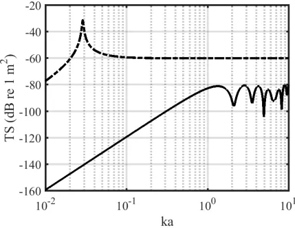
1.1 Target strength gas bubbles (dashed line) and oil droplets (solid line)
accord-ing to Anderson (1950) as function of the size (a) and acoustic wave number
(k). . . 4
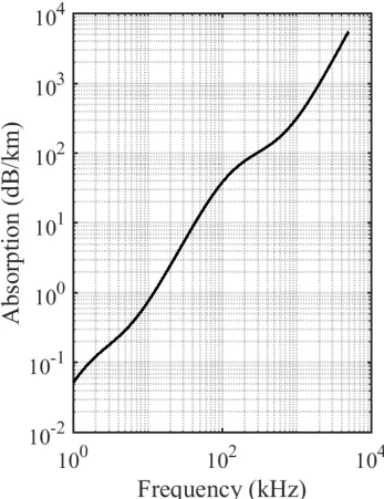
1.2 The absorption as a function of frequency for sound waves at 20 ◦ C and 40 meters water depth according to Francois & Garrison (1982). . . 10
2.1 Comparison of literature sound speed data and BW92 model as a function of
(A) temperature and (B) pressure. Residuals are the difference between the
literature sound speed and BW92 in m/s. . . 18
2.2 (A) Exploded exterior view of sound speed chamber with: (I) The
piezo-electric sandwich, (II) the endcaps, and (III) the fill and pressure ports. (B)
Cross-sectional view of interior of sound speed chamber with same labeling as
(A) with the addition of (IV) the hole through which the wires to the
piezo-electric “sandwich” pass. (C) The piezoelectic sandwich. The brass washers
(i) are wired to the signal generator, with one washer wired to positive and
the other to negative. These washers sit flush against the face of the
piezo-electric transducer (ii). The washers and held apart and the entire sandwich
held together by the plastic spacers (iii) which also fit flush against the inside
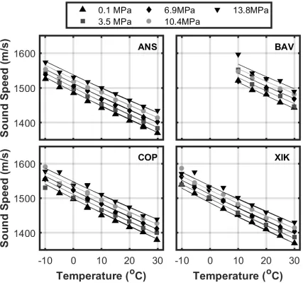
2.3 Diagram of sound speed chamber temperature and pressure control and data
collection. . . 22
2.4 Sound speed of type 1 deonized water measured (markers) compared to
Bel-ogol’skii et al. (1999) (lines). . . 24
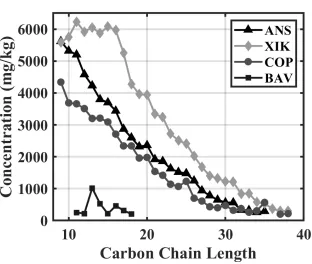
2.5 Concentration of saturated hydrocarbons by carbon chain length. . . 26
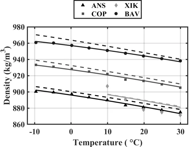
2.6 Density results comparing measured (markers), empirically derived model in
this study (solid lines) and BW92 (dashed lines). . . 27
2.7 Measured sound speed (markers) and empirically derived model from this
study (lines). . . 29
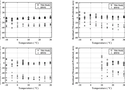
2.8 Residuals for sound speed measured in the present work and newly derived
model compared to residuals for sound speed measured in the present work
and BW92. A.) ANS, B.) XIK, C.) COP, D.) BAV. . . 30
2.9 Residuals between literature values for sound speed and the empirical equation
from this study as well as BW92. A.) Medium Oil, B.) Heavy Oil. . . 33
2.10 Acoustic scattering predicted by Anderson (1950) using the measured impedance
(dotted line), impedance predicted by BW92 (dashed) and impedance
pre-dicted by the empirically derived model in this study (solid line) for a COP
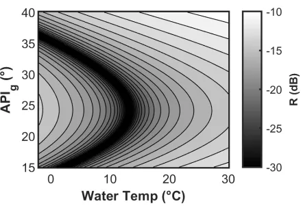
droplet at 25◦C. . . 34 2.11 Reflection coefficients for an acoustically smooth water-oil interface as a
func-tion of API gravity and temperature assuming that the oil and water
temper-atures are at equilibrium (Clay & Medwin, 1977). The acoustic properties of
the oil are determined by the empirically derived model (Eqs. 2.5 and 2.6) at
atmospheric pressure and the water has a salinity of 30 psu. Local minima
in the reflection coefficient curve highlight the combinations of oil and
wa-ter properties that would make the detection of thin oil layers difficult using
2.12 (A) Raw waveform showing the return from the shorter side and the lower
amplitude return from the second side. (B) Autocorrelation of (A) with times
used to calculate sound speed labeled. . . 40
3.1 Geometry of incident wave, (~ki)t, and an oblate oil droplet for end-on
ensoni-fication for use in the DWBA. r~pos is the position vector and a(r~pos) is the
radius of cylinder of thickness d ~rpos, at position r~pos. . . 49
3.2 Geometery of incident wave,pinc, on a droplet Ω with surface Γ. Γ is divided
into surface elements a location mathbf xi with vector normal to the element
surface n. The incident wave travels parallel to the axis of symmetry of the
oblate spheroidal droplet. . . 50
3.3 a. Top down view and b. side on perspective of droplet making and imaging
system. 1: High definition machine vision camera. 2: Needle rosette. 3:
Cali-bration target. 4: Stepper motors. 5: Oil Reservoir. 6. LED light panel. The
stepper motors on the camera platform move the camera in two dimensions
parallel to the bottom of the platform. The camera is moved perpendicular to
the face of the calibration target to focus on the plane containing the target
and needle. The camera is then moved from the calibration to the target to
the needle rosette. pinc indicates the direction of the incident wave from the
echo sounders at the tank surface. . . 54
3.4 a: Image processing example for oil droplet. Droplets are released at a rate so
that only a single droplet is in frame. b: Zoom in on the droplet from A with
the outline of the assumed oblate spheroid shape overlaid (cyan line) showing
3.5 Grouped major radius results for XIK. a. Sorted major radii for all droplets
(red circles) organized into 100µmwide groups (black boxes) with group
num-ber labeled, showing the uneven distribution of radii across the size range and
within groups. b. Distribution of radii measurements in group four showing
the approximately normal distribution of droplets within a group. The mean
(red dashed line) and 95% confidence intervals (blue dotted line) are shown. 57
3.6 Frequency response for a single ANS droplet of equivalent radius 2.93 mm.
Gray crosses are from individual pings, and the black line is the mean intensity
calculated at each frequency in dB. The dotted lines indicate the noise floor
of the three transducers. . . 62
3.7 Recorded scattering (red circles) compared to Anderson 1950 (dashed gray
line), DWBA (solid gray line) and BEM (dotted black line). (a)ANS:
Equiv-alent radius: 2.68mm (b)XIK:Equivalent radius: 3.07mm (c) BAV:
Equiv-alent radius: 4.65mm . . . 63
3.8 Peak amplitude of the measured TS compared to the peak of (a) Anderson
(1950), (b) the DWBA, and (c) the BEM. ANS (dark gray diamonds), XIK
(light gray squares), and BAV (black circles) are compared to unity (black
line). The RMS error between all measurements and the modeled peak is
listed for each model. . . 65
3.9 Frequency of the null in ANS for measured (black circle) and modeled (gray
x) TS according to (a) Anderson (1950), (b) DWBA, (c) BEM. The null
frequency for models computed at the 95% confidence limits of droplet size
are indicated by bars above and below model markers. Gray boxes show the
gap in ensonified frequencies between transducers. For recorded data, nulls
detected within 10 kHz of the gap in frequencies between transducers are
3.10 Frequency of the null in XIK for measured (black circle) and modeled (gray
x) TS according to (a) Anderson (1950), (b) DWBA, (c) BEM. The null
frequency for models computed at the 95% confidence limits of droplet size
are indicated by bars above and below model markers. Gray boxes show
the gap in ensonified frequencies between transducers. For recorded data,
nulls detected within 10 kHz of the gap in frequencies between transducers
are excluded. Note that no nulls were detected for the measured TS of the
smallest XIK droplet. . . 67
3.11 Frequency of the null in BAV for measured (black circle) and modeled (gray
x) TS according to (a) Anderson (1950), (b) DWBA, (c) BEM. The null
frequency for models computed at the 95% confidence limits of droplet size
are indicated by bars above and below model markers. Gray boxes show the
gap in ensonified frequencies between transducers. For recorded data, nulls
detected within 10 kHz of the gap in frequencies between transducers are
excluded. . . 68
3.12 % Error in the estimated droplet volume of a droplet when using the null
frequency to determine droplet size with (a) Anderson (1950), (b) the DWBA
and (c) the BEM for ANS (dark gray diamonds), XIK (light gray squares),
and BAV (black circles). . . 71
4.1 The predicted target strength (TS) of gas bubbles and oil droplets. The
target strength for a methane bubble of radius 0.65 mm (solid black line) and
a bubble with radius 0.28 mm (grey dashed line) show the distinct resonance
peak and high amplitude scattering at low frequencies typical of gas bubbles.
A 3.0 mm radius droplet (grey solid line) and 1.2 mm radius droplet (black
dashed line) show a much lower target strength at low frequencies and the
4.2 ADCP and WBT Survey locations; WBT cross sectional survey lines run
perpendicular to the nominal flow direction (blue), WBT down-stream survey
lines run parallel to flow (black) and ADCP survey lines run perpendicular
to flow (green). Most WBT lines were run downstream of the plume origin
(red o). The red dots show the location of the echograms in Fig 4.3, where
echogram A is the cross sectional pass closest to the origin, echogram B then
next farthest and D is the cross sectional pass farthest from the origin of the
echograms shown. Echogram A is the first pass where the entire plume was
within the range of the ADCP data and it shows a cross section of the plume
as well as the platform lying on the seafloor. Echograms B-D show the two
separate seeps at shallow depths. . . 78
4.3 Echograms for cross sectional passes downstream of the northern seep origin
(see Plume Origin section) at the locations shown in Fig 4.2. (a) is the
echogram closest to the origin (58 m), followed by (b) (115 m) then (c) (187
m) and (d) is the cross sectional pass furthest from the northern seep origin
(235 m) of the four echograms shown here. . . 79
4.4 Down-stream WBT survey echograms for lines run parallel to flow. These
are examples of two of eight lines run parallel to the nominal direction of
flow connecting the locations of the plume determined by the cross section
survey. The downed platform is visible on the seafloor. The black box shows
the area of the echogram used to determine the origin of seeps. In echogram
a, the plume was out of the beam for horizontal distances between 190 and
220 meters, due to variation in the current direction and position of the vessel
during down-stream passes. . . 81
4.5 The orientation of the beams of the ADCP. The ADCP is pointing towards
the bow of the vessel and is on the port side of the vessel in this image. The
4.6 ADCP survey results. (A) the magnitude of the current for the survey run
before the WBT survey (grey dashed line) and ADCP survey run after the
WBT survey (grey dotted line). The last good depth of the ADCP for the
survey before the WBT survey was 95.2 meters and 77.2 meters for the ADCP
survey after the WBT survey. The two surveys were averaged together to
estimate the current over the WBT survey period (black sold line) for depths
less than 77.2 m. For greater depths the pre-WBT survey measurements were
used. (B) the direction of the flow as a function of depth varied by about
15 ◦ for most the water column for the surveys conducted before the WBT survey (grey dashed line), after the survey (grey dotted line) and the mean of
the two surveys (solid black line). At depths measured only by the pre-WBT
survey, there appears to be a low magnitude current to the southeast, about
90◦ offset from the upper water column. . . 86 4.7 Linear interpolation of the TS averaged over 108 - 113 m depth for the area
surrounding the downed platform. The black triangles indicate origins of
the two seeps. The origins are the areas of maximum backscatter at depths
immediately above the downed platform. The platform itself masked the
return from the seep at depths below 113 m. Contour lines are equal a change
of 3 dB. . . 87
4.8 A. A zoomed in version of the echogram in Figure 4.3D focused on the seeps.
B. The phase angle for the seeps as the vessel crosses over them. The angle
goes from negative to positive as the seep transitions across the beam, and
then the transition from negative to positive repeats for the second seep.
Combined with the seep origin analysis, this indicates the presence of two
4.9 The visually picked top (black triangles) and bottom (black squares) of the
plume at distances from the first pass over the plume where the plume was
above the last good depth of the ADCP. The depth of a target as a function
of distance from the first pass account for the depth dependent current for a
target rising with a rise rate of 23.2 cm/s (solid black line), 12 cm/s (dotted
black line), and 6.7 cm/s (dashed black line). The plume extents and target
trajectories are overlaid on the TS ( ˆT S) averaged in a 3 meter depth bin and
for all pings containing the plume at each perpendicular pass. The letters,
to the right of the integrated TS column they represent, correspond to the
echograms in Fig 4.3. . . 89
4.10 The rise rate and target radius predicted by Zheng and Yapa (2000) for
oil droplets (dashed line) and methane bubbles (solid line) in seawater at a
depth of 40 meters. The maximum predicted rise rate for droplets was 0.113
m/s which equates to a 2.82 mm radius droplet, and 0.49 mm bubble. The
minimum rise rate determined from the fit to the echo sounder data was 0.063
m/s which equates to a 1.17 mm droplet and a 0.29 mm bubble. The maximum
rise rate from the fit to the echo sounder data was 0.216 m/s, equivalent to a
1.16 mm bubble. . . 94
4.11 a. an echogram of the 104 pings used in the noise calculation showing the
stratified water column. b. Noise profiles for the minimum frequency (94
kHz, gray) and maximum frequency (153.5 kHz, black) average into 0.5 meter
4.12 A section of the echogram in Fig 4.3A zoomed in to the plume area. The
black boxes outlines the area of the plume predicted to contain oil droplets.
Targets in this area rose with a rise rate equal to or less than 11.3 cm/s. The
white box outlines the area of the plume predicted to contain gas bubbles.
There is no predicted maximum or minimum rise rate for methane bubbles
according to (Zheng & Yapa, 2000) and therefore the entirety of the plume is
predicted to potentially contain gas bubbles. . . 98
4.13 The measured frequency dependant target strength (σtgray dots) compared to
the predicted backscatter for the scenario where all targets are methane
bub-bles (σbs,NN, solid black line) and where all targets are oil droplets (σbs,MM,
black dashed line) for a single cross sectional pass. (a) is a rise rate of 20.2
cm/s and bubbles radius 1.04 mm, (b) is a rise rate of 10.3 cm/s, bubble
ra-dius of 0.45 mm and droplet rara-dius 2.24 mm and (c) is a rise rate of 6.9 cm/s,
bubble radius 0.31 mm and droplet radius 1.33 mm. There are no droplets
predicted for (a) because it is in the bubble rise rate regime - the rise rate is
greater than the maximum predicted bubble rise rate (11.3 cm/s). The black
dotted line is the noise level,σbg, for the same depth as the targets. . . 99
4.14 The depth integrated flow rate of oil for each cross section of the plume by
distance from the northern seep origin. . . 100
4.15 The depth integrated volumetric flow rate of methane for each cross section of
the plume by distance from the northern seep origin for both rise rate regimes
(Black circles) and the oil droplet rise rate regime only (black crosses). The
fit lines are also shown for both rise rate regimes (solid black line) and the oil
4.16 The total methane and oil volumetric flow rate from the droplet rise rate
regime (rise rate ¡ 11.3 cm/s) required to explain the acoustic observations in
that regime for different GOR’s. The GOR is the ratio of the volume of gas
in the entire plume to the volume of oil in the entire plume. The entire plume
includes both the droplet rise rate regime and the bubble rise rate regime,
however oil is predict to only be present in the droplet rise rate regime. When
the total volume of the droplet rise rate regime is assumed to be oil droplets,
the GOR of the entire plume is approximately 1. . . 101
5.1 The frequency response for a 1 mm (solid black line) and 3 mm radius (dashed
line) ANS droplet at 20◦C and hydrostatic pressure deteremined at depth. The red asterix indicate the peak of the backscatter in the broadband range of the
ES120 and ES333 described in chapter 3. . . 107
5.2 The percent of oil per volume of seawater require for detection as a function
of range at 120 kHz (solid lines) and 333 kHz (dashed line) for 1 mm droplets
(gray lines) and 3 mm droplets (black lines). The detection ranges are
com-puted for environments with noise equal to the (a) the noise level averaged
between 40 and 60 meters (Fig.4.11b) and (b) is the detection range for the
Scott Loranger
Abstract
The fate and transport of oil droplets from natural and anthropogenic sources is key to
under-standing the impact of spills and the resilience of marine communities. Without knowledge
of natural background levels, it is difficult to determine the response of the marine
envi-ronment to large influxes of oil. Current estimates of global flux of oil from natural seeps
varies by an order of magnitude, and the wide range of estimates is due in part to the lack of
sufficient in-situ quantification techniques for oil droplets in the water column. This work is
focused on the feasibility of employing broadband acoustics to address this gap by developing
a better understanding of the interaction between sound generated by broadband acoustics
and oil droplets in the ocean. The dissertation is organized into three experiments, each
written into a manuscript for peer-reviewed publication. The first addresses the paucity of
data at oceanographically-relevant pressures and temperatures regarding the physical
prop-erties of crude oil that impact acoustic scattering. The acoustic impedance of four crude
oils was measured under oceanographic conditions using a sound speed chamber designed
and constructed for this experiment. Measurements showed significant deviations from an
often-used empirical model and a new empirical model was developed. The results of the
first experiment were used in the analysis of the second study. High frequency broadband
acoustic backscatter was recorded from droplets of three different crude oils of varying size
and shape and compared to three scattering models for fluid targets. The results highlighted
the importance of droplet shape (i.e., deviations from a perfect sphere) in acoustic
backscat-ter observations of crude oil droplets. The first two experiments were used to inform the
analysis of the third experiment. Broadband acoustics along with ADCP measurements were
Introduction
1.1
Background
It is estimated that over 2 million tons of oil enters marine environments from anthropogenic
sources annually (GESAMP, 2007). Anthropogenic oil spills can have devastating impacts
on marine organisms that cascade across trophic levels. For example, within the planktonic
community an influx of hydrocarbons can have drastically different effects across species
(Abbriano et al. , 2011). Certain species of hydrocarbon specialists will experience blooms
following a spill event (Transportation Research Board and National Research Council, 2003;
Valentineet al. , 2010), while other species will experience significant declines (Ozhanet al.
, 2014). A study by Parsonset al. (2015) found that during the Deepwater Horizon spill the
phytoplankton community as a whole decreased in abundance and that there was a significant
shift in the community composition. At higher tropic levels the combined impacts of changes
to the planktonic community assemblage and the effects of direct exposure to hydrocarbons
result in significant changes including increased mortality and decreased fecundity (Beyer
et al. , 2016). Increased oil concentrations in the marine environment impact economically
important species including shrimp (Van Der Ham & De Mutsert, 2014), predatory pelagic
the impacts are highly variable and depend on the hydrocarbon concentrations experienced
locally which can vary over small spatial scales within the spill area (Rozas et al. , 2000;
Mendelssohn et al. , 2012).
Oil spill responders use the best available technology and science to respond to spills and
mitigate environmental and economic impacts, however, they are often hampered by a lack
of real timein-situ data on the fate and transport of oil, especially from seafloor hydrocarbon
sources. Oil spills cover massive areas with hydrocarbon concentrations varying locally on
scales of tens of meters. The most efficient and effective response to a spill would be to
determine where the impacts will be greatest and use the available response resources in those
areas. However, withoutin-situ oil detection and quantification techniques, especially in the
water column, responders do not have the information they need to adequately determine
what areas are likely to be the most significantly impacted. The work presented in this thesis
describes novelin-situ acoustic methodologies developed for the detection and quantification
of oil in the marine environment to address this critical gap in knowledge.
The lack of in-situ measurements of oil leads to many unanswered questions about the
environmental response to influxes of oil - both anthropogenic and natural - across the
climatically and ecologically diverse environments that are exposed to hydrocarbons.
Un-derstanding potential environmental impacts due to spills and developing an appropriate
response requires both the ability to quantify the total volume of oil spilled and knowledge
of baseline levels of natural oil seepage. Current estimates of the global flux of oil from
nat-ural sources varies by an order of magnitude (Transportation Research Board and National
Research Council, 2003) and this uncertainty in background levels results in uncertainty of
the potential impacts of a spill on the environment. For example, the Deepwater Horizon
spill was an influx of between 34 - 340% of the total annual flux from natural sources in
the Gulf of Mexico (United States & Coast Guard, 2011). While any increase above
back-ground levels is likely to have an environmental impact, knowledge of the magnitude of a
response and to assess the long-term impact on the environment. Acoustic methods offer
a path toward quantifying both anthropogenically released and naturally occurring liquid
hydrocarbons in the ocean.
Active acoustic methods have been used to estimate the flux of oil from seafloor wells
(Camilli et al. , 2012), to determine flux of oil at ranges of up to a hundred meters from
the instrument (Weberet al., 2012) and to estimate the thickness of oil layers under sea ice
(Wilkinsonet al. , 2015; Bassettet al., 2016; Pegau et al., 2017). The main impediment to
the use of acoustic methods for detection and quantification of oil is the low characteristic
acoustic impedance contrast between crude oil and seawater. The contrast in the
character-istic acoustic impedance (the product of the density and sound speed) determines the degree
to which sounds is reflected and refracted at the boundary between two media; in this case
the boundary of the ambient seawater and the oil droplet. While the acoustic impedance
of oil is poorly understood at oceanographic conditions (see Chapter 2), it is sufficiently
characterized to determine that the impedance is similar to that of water, and to therefore
classify oil droplets in the ocean as weakly scattering.
Weakly scattering particles such as oil droplets reflect the most sound when the
wave-length of the sound wave (λ) is of the same size or smaller than the radius of the particle
(a), a situation referred to as geometric scattering. The relationship between wavelength
and particle size is typically expressed in terms of ka where k is the acoustic wave number
(2π/λ). When ka is less than one, described as Rayleigh scattering, the efficiency of
scat-ter, or target strength (TS), for a weak scattererer decreases with a power law that goes
as (ka)4a2 (Figure 1.1). TS is the ratio of the intensity of the backscattered sound to the
intensity of the incident sound, and is therefore a measure of the efficiency of backscatter
of a particle. Gas bubbles, which have a larger characteristic acoustic impedance contrast,
are much better scatterers of sound and have a higher TS across all frequencies than an oil
droplet of the same size. Wavelength is inversely proportional to frequency and low frequency
Figure 1.1: Target strength gas bubbles (dashed line) and oil droplets (solid line) according to Anderson (1950) as function of the size (a) and acoustic wave number (k).
shows the TS as a function of frequency for a one mm droplet according to the exact modal
solution for a plane wave incident on a fluid sphere derived by Anderson (1950). For a 1 mm
radius oil droplet, the transition from Rayleigh to geometric scattering occurs at around 240
kHz, and Figure 1.1 shows the decrease in TS at frequencies below 240 kHz. During the
Deepwater Horizon spill Weberet al. (2012) were able to detect oil at distances greater than
100 meters with a 200 kHz shipboard echo sounder, however they were unable to detect oil
at lower frequencies, where ka was much less than one.
The higher frequencies associated with the geometric scattering regime for oil droplets
are also associated with increased signal attenuation (Figure 2). Absorption in seawater is
frequency echo sounding to short ranges. There is a trade off in determining the frequency
most appropriate for detecting oil droplets, frequencies should be high enough so thatka is
around one but also low enough to mitigate signal attenuation due to absorption. One way
to increase the signal to noise ratio (SNR), and therefore increase the range of detection,
is to use a broadband acoustic signal. The acoustic waveform recorded by a broadband
echo sounder can be matched-filtered, where the recorded signal is cross-correlated with the
broadband transmit signal. A broadband matched-filter improves the SNR by approximately
2BT where B with the bandwidth of the signal and T is the pulse length (Turin, 1960; Chu
& Stanton, 1998; Stanton & Chu, 2008; Lavery et al. , 2010; Stantonet al. , 2010).
The added benefit of using a broadband signal is that the broadband frequency response
can be used to estimate the physical properties of a target. Backscattering measured at
single frequency only reveals a point on the frequency response curve for a target, but when
a wide range of frequencies is used the shape of the frequency response reveals information
about the target. Previous work has used the broadband backscatter frequency response
to differentiate between plankton and turbulent microstructure (Lavery et al. , 2010), to
quantify bubbles under breaking waves (Medwin & Breitz, 1989; Terrill & Melville, 2000;
Vagle & Farmer, 1992), and as an aid for classifying fish species (Holliday, 1972; Thompson
& Love, 1996; Stanton et al. , 2010). The backscattering frequency response (Figure 1.1)
for oil droplets is dependent on the droplet’s impedance, size and shape. Therefore, if
the impedance and shape are known, the frequency response can be used to estimate the
remaining physical property; droplet size. In order to use the frequency response to quantify
the physical properties of a target, some structure in the frequency response, such as a peak,
null or change in slope, needs to be measured. The broader the transmitted signal, the more
likely it is that a structure such as a null (or more ideally multiple nulls) will be within
the ensonified range. In order to quantify droplets with broadband signals, the accuracy of
acoustic scattering models, and the assumptions made in such models, for oil droplets must
Two potential impediments to the use of broadband acoustics for quantifying oil droplets
come from other scatterers present at oil seeps; gas bubbles and biological scatterers (Judd,
2003; Sahlinget al. , 2016; Kvenvolden & Cooper, 2003). Oil seeps, whether anthropogenic
or natural, are often co-located with hydrocarbon gas bubbles. As discussed previously, gas
bubbles have a higher impedance contrast with seawater than oil droplets and therefore are
more efficient at scattering sound (Figure 1.1). When gas bubbles and oil droplets are in
the same ensonified volume gas bubbles will mask any response from oil droplets, unless the
oil is present in very high concentrations relative to the gas. Most planktonic organisms, on
the other hand, are modeled as weak scatterers, just like oil droplets. Layers of planktonic
organisms in the water column can mask oil droplets completely if present in dense enough
layers. When concentrations of oil and gas are similar the TS of the biological scatterers can
combine with the TS from oil droplets and suppress the peak and null shape used to quantify
droplets when present in the same ensonified volume. While it is possible to quantify oil
droplets under ideal laboratory conditions (see Chapter 3) at a field site where biological
scatterers and gas bubbles are also present, quantification of oil will be more difficult (see
Chapter 4).
The work presented in this thesis seeks to expand our understanding of how sound
inter-acts with oil droplets in an effort to develop acoustic methodologies that will improve our
understanding of the fate and transport of oil in the marine environment. The thesis consists
of three studies of increasing spatial scale; a bench-top study of the physical properties of
crude oil that determine scattering, a mesoscale laboratory study of the broadband
scatter-ing from individual oil droplets and a field evaluation of the use of shipboard broadband
echo sounders to detect and quantify oil from a seafloor seep.
The study in Chapter 1 focused on the physical properties of oil that determine acoustic
scattering at oceanographic conditions. In order to understand how sound interacts with oil
droplets researchers need to know how the characteristic impedance - the density and sound
results of chapter 1 to inform scattering models of oil droplets and compares the predictions
of those models to empirical measurements of backscatter. In order to determine the physical
properties of oil droplets - most importantly the droplet size - acoustically researchers need
to know that models of acoustic backscatter from oil droplets are accurate and precise. If
the sound speed and density of oil droplets is known, it should be possible to determine
droplet size acoustically. In Chapter 2, the broadband backscattering frequency response of
oil droplets of varying and known size from three of the four oils studied in chapter 1 was
measuredin-situ. Three commonly used models for backscattering of fluid targets were then
inverted for droplet size. The size measured empirically and the size predicted by the models
was compared to determine the accuracy of inversions of those models. Chapter 3 then used
the models verified in Chapters 1 and 2 to predict the scattering from oil droplets emanating
from a seafloor seep source in the Gulf of Mexico. Droplet size was predicted by the rise rate
of droplets determined acoustically. The droplet size predictions were combined with sound
speed and density modeled by the results of Chapter 1 and used to predict the frequency
response of oil droplets using a model verified in Chapter 2. The frequency response was
then compared to the measured backscatter to determine the flux from the seep site.
The research questions, significance, hypotheses, and outcomes of the three chapters are
outlined below.
Chapter 1.) Acoustically relevant properties of four crude oils at
oceano-graphic temperatures and pressures
Question: Do oceanographic conditions cause significant deviations for the generally
accepted model of the physical properties of oil, a model that is derived from measurements
made at reservoir conditions?
Significance: Empirical models of density and sound speed, the properties that determine
acoustic scattering, are derived from measurements of those properties made at reservoir
conditions (very high temperature and pressure). At oceanographic conditions the waxes in
Hypothesis: The formation of waxes in crude oils at oceanographic conditions will cause
significant deviations between the measured density and sound speed and the density and
sound speed predicted by the commonly used empirical model.
Outcomes: Significant deviations between measured and modeled sound speed and
den-sity were found at oceanographic conditions and a new empirical model for those properties
at oceanographic conditions was derived. The new empirical model outperformed the
com-monly used model when compared to sound speed measurements from the literature.
2.) Broadband acoustic scattering from oblate hydrocarbon droplets
Question: Do currently used models of acoustic scattering from oil droplets accurately
predict the backscatter from individual droplets accurately enough to quantify droplet size?
Significance: In order to quantify oil droplets with broadband acoustics, models of
backscatter must accurately characterize the broadband backscattering frequency response,
especially the peak and null structure of the acoustic backscatter to differentiate between
droplet sizes. Previous work has assumed droplets are spheres and if this assumption is
vio-lated the use of sphere models is likely to cause significant errors when inverting scattering
models to determine droplet size.
Hypothesis: Models that assume oil droplets are spherical will not accurately predict
the frequency dependent backscatter of droplets that are non-spherical. Other models that
account for more complex shapes will show better agreement between the peak and null
shape of the TS and the shape of the TS measured experimentally.
Outcomes: A model for acoustic scattering from fluid spheres did not accurately predict
the null location of droplet of known impedance, shape and size. The distorted wave Born
approximation and boundary element method, models that account for more complex shapes,
showed better agreement for medium oils between the predicted and measured null location
and inversions of those models accurately predicted the droplet size within the accuracy of
the experimental system. However, there were significant errors when using inversions of
3.) Hydrocarbon detection and quantification at a marine oil and gas seep
Question: Can a shipboard broadband acoustic echo sounder determine the flux of oil
from a seep site known to consistently be producing an oil slick in the Gulf of Mexico?
Significance: Shipboard broadband acoustics were deployed in the presence of gas bubbles
and biological scatterers to determine the flux of oil in-situ from a seep site in the Gulf of
Mexico. The determination of flux in the water column in-situ is a new tool in the oil spill
responder toolkit that can be used to detect and quantify oil from greater distances then
current detection methods.
Hypothesis: Broadband acoustic backscatter will be able to detect and quantify oil
droplets from a seafloor seep site and distinguish between the droplets, biological scatterers
and hydrocarbon gas bubbles present at the site. The results will be a determination of the
flux from a seafloor seep using shipboard acoustics.
Outcomes: The shipboard echo sounder was able to quantify the flux of methane and
oil from the seep site. The plume at this site was divided into two regions - a high rise
rate region where it was assumed only gas bubbles had a sufficiently high rise rate to be
present, and a lower rise rate region likely to contain oil droplets and gas bubbles. For the
end member assumption that all the targets in the droplet rise rate regime were oil droplets
flux was between 156 - 341 barrels per day at the 95% confidence interval with a mean
of 249 barrels per day. If that same region was comprised solely of methane gas bubbles,
flux was 3.84 - 13.7 m3 /day with a mean of 8.78 m3 / day. The flux for increasing gas to
oil ratios (GOR) were also computed. In order to estimate the GOR from the broadband
acoustic backscatter, as outlined in chapters 2 and 3, accurate measurements of the material
properties of the oil and gas at the site is required. Measurements of these properties were
Acoustically relevant properties of
four crude oils at oceanographic
temperatures and pressures
Scott Loranger1, Christopher Bassett2, Justin P. Cole3, Bret Boyle3, and Thomas C.
Weber4
1 Department of Earth Sciences, University of New Hampshire, Durham, NH 03824
2National Marine Fisheries Service, Alaska Fisheries Service Center, Resource Assessment and
Conservation Engineering Division,Seattle, WA 98115, USA
3Department of Chemistry, Colorado State University, Fort Collins, CO, 80526
4Department of Mechanical Engineering, University of New Hampshire, 105 Main Street,
Abstract
Inversions of models of broadband acoustic scattering to detect and quantify weakly
scattering targets, such as oil droplets in seawater, require precise knowledge of the physical
properties that determine scattering. When the characteristic impedance contrast between a
target and the surrounding medium is weak, small differences between the true and modeled
impedance can cause significant errors in modeled scattering. For crude oil, currently
avail-able empirical models of density and sound speed are derived from measurements made at
reservoir conditions (high temperature and pressure), which may not be relevant to
oceano-graphic conditions due to phase changes in the oil. Measurements of the density and sound
speed, as well as thermal characterization of phase changes via differential scanning
calorime-try, of four crude oils at oceanographically relevant temperatures and pressures were made
and compared to a commonly used empirical model for sound speed and density. Significant
deviations between the measured and modeled values were found and new empirically fit
models were developed. A literature review of sound speed data was also performed, and
the new empirical model shows improvement over the commonly used empirical model for
2.1
Introduction
At the end of the first quarter of 2018, almost 800 offshore drilling rigs were available
for hydrocarbon extraction (IHS, 2015). Over the past decade offshore oil production has
accounted for approximately 30% of total oil production (U.S. Department of Energy, Energy
Information Administration, 2016). Advances in exploration and extraction technology have
resulted in expansion of offshore production into new environments. While a majority of this
oil is extracted from waters less than 125 m deep, increasingly large portions are extracted
from depths in excess of 1,500 m. This production occurs globally with rigs located in
areas that cover the full range of oceanographic environments from warm tropical waters to
seasonally ice-covered waters in the Arctic.
Many questions exist about the expected environmental impact of spills in the
climati-cally and ecologiclimati-cally diverse environments where drilling occurs. Understanding potential
environmental impacts due to spills and developing an appropriate response requires both the
ability to quantify the total volume of oil spilled and knowledge of baseline levels of natural
oil seepage. For example, the Deepwater Horizon spill released approximately 680,000 tonnes
of oil (United States & Coast Guard, 2011). The most recently available estimate of annual
flux of liquid hydrocarbons from natural seepage in the Gulf of Mexico is between 80,000
tonnes and 200,000 tonnes of oil and between 200,000 tonnes and 2,000,000 tonnes worldwide
(Transportation Research Board and National Research Council, 2003). Liquid hydrocarbon
flux from the Deepwater Horizon spill is estimated to have been between 34% and 340% of
the global annual flux of oil into the ocean. While any increase above background levels
is likely to have an environmental impact, knowledge of the magnitude of a spill relative
to background levels is necessary both to inform decision making during spill response and
to assess the long-term impact on the environment. Acoustic methods (e.g., Camilli et al.
(2012), Weber et al. (2012)), offer a path toward quantifying both anthropogenically
re-leased and naturally occurring liquid hydrocarbons in the ocean, but are limited by the
models at oceanographic conditions. The present work seeks to address this information gap
by reporting measurements of oil density and sound speed under pressure and temperature
conditions relevant to much of the worlds oceans, and by developing an empirical model for
these properties that performs better than existing models for the types of oils studied.
Natural hydrocarbon seepage from the seafloor can take the form of free gas,
hydrate-coated gas bubbles, and liquid oil, and occur throughout the worlds’ oceans (Judd, 2003;
Sahling et al. , 2016; Kvenvolden & Cooper, 2003). Seepage associated with free gas (with
or without hydrate) is often detected and quantified acoustically, taking advantage of the
large impedance contrast between free gas and seawater (Merewetheret al. , 1985; Greinert
et al. , 2006; Heeschen et al. , 2003; Schneider von Deimling et al. , 2011; R¨omer et al.
, 2012; Weber et al. , 2014). The present study is aimed at the study and assessment of
the seepage of liquid oil, such as the seeps reported in the Gulf of Mexico and the Congo
Basin (Transportation Research Board and National Research Council, 2003; Crooke et al.
, 2015; Roberts & Carney, 1997; Sahling et al. , 2016; Jatiaultet al. , 2018). In deep water
environments a variety of instrumentation is used for the detection and quantification of
oil, however, most of these instruments are limited to short detection ranges on the order
of meters, or even centimeters (e.g., fluorometers, mass spectrometers). Given this short
detection range it is difficult to accurately evaluate the flux for an entire ocean basin, or
even a large spill. Acoustic instrumentation provides the potential for the detection and
quantification of hydrocarbons at greater ranges. Active acoustic methods have been used
to estimate the flux of oil from deep-water blowouts (Camilli et al. , 2012), to detect and
quantify oil at ranges of up to hundreds of meters from the instrument (Weberet al. , 2012),
and to estimate the thickness of oil layers under sea ice (Wilkinson et al. , 2015; Bassett
et al. , 2016; Pegau et al. , 2017).
Quantifying oil acoustically, whether present as droplets or in layers, depends on a
thor-ough understanding of the physical properties that determine acoustic scattering. The
or shape of a droplet) and the mismatch between the characteristic impedance (the product
of density and sound speed) of the surrounding water and the target. In previous studies of
crude oil researchers have had to make assumptions about the physical properties of oil in
order to estimate flux (Weber et al. , 2012).
One of the reasons that the acoustically-relevant properties of crude oil (shape, size,
den-sity and sound speed) are difficult to quantify is that the term “crude oil” encompasses a
wide variety of unrefined liquid petroleum products that are composed of multiple
hydrocar-bon chains of different molecular weights, in addition to other organic materials. Crude oils
are often classified by their American Petroleum Institute gravity, APIg. This dimensionless
quantity is related to the specific gravity of the liquid according to APIg = 141SG.5 −131.5,
where SG is the specific gravity of the liquid at 15.56 ◦ C and 0.1 MPa. By this definition light crudes have an APIg higher than 31.1◦, medium crudes APIg between 22.3 ◦ and 31.1
◦, and heavy to extra heavy crude oils have an API
g less than 22.3 ◦. The concentration of hydrocarbon chains of differing length and geometry as well as organic material present
generally varies based on the origin of the petroleum and oils with similar APIg do not
necessarily have the same distribution of hydrocarbon chains and organic materials.
The saturated hydrocarbon chains (also referred to as paraffins, waxes or n-alkanes),
which generally make up a significant percentage of the mass of crude oil, are prone to
crystallization at temperatures and pressures lower than those found in oil reservoirs. As
temperature decreases, the temperature at which the saturated hydrocarbons begin to change
phase from liquid to solid is referred to as the wax appearance temperature (WAT). In
general, as molecular weight of saturated hydrocarbons increases the temperature at which
saturated hydrocarbons come out of solution as solids increases (Garc´ıa & Urbina, 2003). The
WAT is also determined by the breadth of distribution of paraffins, with wider distributions
of carbon chain length resulting in a lower WAT (Garc´ıa, 2000; Ronningsen et al. , 1991;
Vazquez & Mansoori, 2000) Significant changes to the physical properties of oils can occur
properties that determine acoustic scattering at oceanographically relevant temperature and
pressures.
In this study a review of the measurements of sound speed available in the literature was
performed and the results compared to Batzle & Wang (1992), a commonly used empirical
model of the physical properties of oil. Samples of four crude oils were then chemically
analyzed to quantify the concentration of saturated hydrocarbons and phase changes were
identified and quantified by differential scanning calorimetry (DSC) over the relevant
temper-ature range. To adequately characterize oils for acoustic scattering applications, the density
and sound speed was measured over oceanographically relevant temperatures (-10 ◦C to 30
◦C). Sound speed was also measured at oceanographically relevant pressures (0 MPa to 13.79
MPa). Finally, these results were also compared to the Batzle & Wang (1992) empirically
derived model for sound speed and density of crude oils.
2.2
Literature Review
To evaluate the applicability of empirical models derived from measurements of oils at
reser-voir temperature and pressure to oceanographic conditions a literature review of available
sound speed data was performed. Targeted search criteria returned 985 papers. These
pa-pers were further refined by exclusion criteria (Appendix 2.6) designed to eliminate papa-pers
with insufficient data for modeling sound speed. For example, papers that did not include
temperature and/or pressure of measurements were excluded. Following filtering by the
ex-clusion criteria only nine papers made measurements of the sound speed of crude oil with
sufficient data for modeling (Daridon et al. , 1998; Ball et al. , 2002; Meng et al. , 2006;
Georgeet al. , 2008; Hanet al. , 2010; Plantier et al. , 2008; Chaudhuriet al. , 2012; Bassett
et al. , 2016; Khelladiet al. , 2010). Of the measurements in those nine papers only 19.7%
were made at oceanographically relevant temperatures and pressures. While models derived
for phase changes in oils at lower temperatures and pressures limits the potential
applica-bility of these models to oceanographically relevant conditions. The available literature also
focuses primarily on heavy oils; 70% of measurements at oceanographically conditions fell
into this category.
In addition to the potentially limited applicability to oceanographic conditions, many of
the available models and equations of state rely on a priori knowledge of a wide range of
thermodynamic properties of oils (e.g. Gross & Sadowski (2001)). For oil spill responders
and researchers, such thorough examinations of oil properties are often unfeasible due to the
cost of characterization and limited access to large sample sizes. There are, however, simpler
models that require fewer input parameters.
The most widely cited empirical model is Batzle & Wang (1992) (hereafter referred to as
BW92) which empirically derives values for the sound speed and density of oil based solely
on APIg. Because the focus of BW92 was on reservoir conditions, the authors of BW92
limited their analysis of sound speed and density to data that does not include any phase
transitions. Oil density as a function of pressure is determined in BW92 by
ρp =ρo+ (0.00277P −1.61×10⁻⁷P3)(ρo−1.15)2 + 3.49×10⁻⁴P,
(2.1)
whereρP is the oil density in kg/m3at pressureP in MPa,ρois the oil density at atmospheric
pressure and 15.56◦C (APIg conditions). Temperature is accounted for according to
ρP,T =
ρp
[0.972 + 3.81×10⁻⁴(T + 17.78)1.175], (2.2)
where ρP,T is the oil density as a function of pressure and temperature, T, in ◦C.
Figure 2.1 shows the residuals between BW92 and the sound speed data from seven of
Figure 2.1: Comparison of literature sound speed data and BW92 model as a function of (A) temperature and (B) pressure. Residuals are the difference between the literature sound speed and BW92 in m/s.
Khelladi et al. , 2010) did not have APIg or density data for the oils measured and
there-fore were excluded. BW92 overestimates the sound speed of light oils, RMS error = 211
m/s, underestimates medium and heavy oils, RMS error = 57 m/s and RMS error = 60
m/s respectively. BW92 increasingly underestimates the sound speed of heavy oil as the
temperature decreases.
The heavy oil data from the literature shows an exponential increase in sound speed at
temperatures below 20 ◦C that is not predicted by the BW92 model. Han et al. (2010) proposed that this exponential increase was due to a phase transition in the oil that they
qualitatively referred to as the oil becoming “quasi-solid”. The transition to “quasi-solid”
transition is not quantified by Han et al. (2010).
2.3
Materials and Methods
Samples of four different crude were obtained for analysis. The four oils studied are identified
by the geographic region from which they were extracted: Alaskan North Slope (APIg= 28.2
◦), Coal Oil Point, Califonia (API
g = 22.6◦), Angolan Bavuca (APIg = 17.7◦), and Angolan Xikomba (APIg = 24.4 ◦). The abbreviations ANS, COP, BAV, and XIK, respectively, will serve to reference the specific oils when discussing their properties. Based on their
API gravities, ANS, COP and XIK are all medium oils while BAV is a heavy oil. All
oils were analyzed for saturated hydrocarbon concentration, and thermally characterized by
differential scanning calorimetry from −50 ◦C to 50 ◦C. Density was measured at ambient pressure for temperatures from −10 ◦C to 30 ◦C in 5 ◦C increments. Sound speed was also measured from −10◦C to 30◦C in 5 ◦C increments and at pressure from 0.10 MPa to 13.79 MPa in 3.45 MPa increments.
2.3.1
Calorimetry
Differential scanning calorimetry (DSC) was performed on an TA Instruments DSC Q20.
DSC analysis reveals phase changes occurring within oil samples by measuring the heat
flux required to change the temperature of a sample (Wunderlich, 1990). Deviations in the
first derivative of the heat flux as a function of temperature in the test sample reveal the
presence of a phase change over a temperature range. If the slope of heat flux as a function
of temperature is constant over a region, no phase change is occurring. Measurements were
performed by hermetically sealing each sample in an aluminum pan at atmospheric pressure.
2.3.2
Saturated Hydrocarbons
Saturated hydrocarbon analysis (SHC) was performed by Alpha Analytical according to
EPA SW-846 method 8015D (US EPA, 2007). This method uses Gas Chromatography with
Flame Ionization Detector (GC/FID) to determine the concentration of 32 n-alkane
hydro-carbons (saturated hydrohydro-carbons with only single covalent bonds) and selected isoprenoids
for carbon chains from 9 carbons to 40 carbons in length. The method also reports the total
concentration of saturated hydrocarbons along with the total petroleum hydrocarbons.
2.3.3
Density
Density was measured by calibrated hydrometers, FisherSci 11510B and 11510C, according
to ASTM D1298-12b. Approximately 250mL of each was oil transferred at room
tempera-ture into 300mL ungraduated cylinders and sealed with parafilm. The sealed cylinders and
hydrometers were placed in a temperature-controlled incubator, ESPEC BTL-433, which
was set to−10◦C. A NIST certified Omega Ultra Precise Platinum RTD temperature probe (PMA-1/8-6-1/2-TS5; range: −100 ◦C to 250 ◦C, accuracy: 0.15 ◦C ± 0.002 |T|, where
T is the temperature of measurement) connected to a NIST certified Omega High
Accu-racy PT100 Input Thermometer (HH804U; accuAccu-racy 0.05%|T| ) was inserted through the
parafilm into the XIK sample, which had the highest heat capacity over the temperature
range as measured by DSC. Once the incubator temperature was stable, the samples were
given 1.5-hours to equilibrate. XIK reached a stable temperature of −9.8 ◦C after 45 min-utes. Samples then sat for an additional 45-minutes to assure that the entire sample reached
equilibrium. Temperature inside the incubator was constantly recorded by an RBR solo T
Temperature Logger (accuracy ± 0.002◦C) recording at a 1-second sample rate. Hydrome-ters were placed in each sample and allowed to equilibrate for 30 minutes. Each hydrometer
was read and recorded, noting the maximum height of the oil on the hydrometer. Corrections
ture in the chamber was stable, the samples were allowed 1-hour to equilibrate. These steps
were repeated to obtain measurements in 5 ◦C intervals from −10◦C to 30 ◦C.
2.3.4
Sound Speed
Figure 2.2: (A) Exploded exterior view of sound speed chamber with: (I) The piezoelectric sandwich, (II) the endcaps, and (III) the fill and pressure ports. (B) Cross-sectional view of interior of sound speed chamber with same labeling as (A) with the addition of (IV) the hole through which the wires to the piezoelectric “sandwich” pass. (C) The piezoelectic sandwich. The brass washers (i) are wired to the signal generator, with one washer wired to positive and the other to negative. These washers sit flush against the face of the piezoelectric transducer (ii). The washers and held apart and the entire sandwich held together by the plastic spacers (iii) which also fit flush against the inside of the sound speed chamber. (Color Online).
Sound speed measurements were made using a system modified from the design by Dashti
& Riazi (2014). The chamber was vacuum filled to minimize air entrainment in the sample.
stainless-steel chambers (Figure 2.2). The transducer was driven by an Agilent Arbitrary
Waveform Generator, which drives an 10V peak-to-peak, five-cycle, 750 kHz pulse that
travels bi-directionally through the length of each chamber. No tapering window was applied
to the signal. The waves are reflected by the end caps and then return to the transducer. A
Tektronix TBS 1102B Digital Oscilloscope records the voltages associated with the reflected
waves. Data was recorded over a 100 µs window encompassing only the first and second
returns (excluding the transmit pulse and higher multiple returns) with a sample rate of
2.5 MHz. The Tektronix TBS 1102B Digital Oscilloscope records 16 individual wave forms,
coherently averages them together to reduce noise and outputs that average as a single
waveform. For a given temperature and pressure 100 of the outputted waveforms were
recorded.
Figure 2.3: Diagram of sound speed chamber temperature and pressure control and data collection.
Figure 2.3 diagrams the environmental control and data recording set-up for sound speed
measurements. The internal pressure of the system was controlled by a precision pressure
control valve connected to a SCUBA tank. Pressure data was recorded by a NIST certified
Omega Digital Pressure Gauge (DPG409-3.5KG) with and accuracy of 0.08% of the full scale
connected to a PolyScience Programmable Temperature Controller. A 50/50 mixture of
water/ethylene glycol was used as the bath fluid to permit temperatures as low as −50◦C. Temperature in the housing was recorded by a NIST certified Omega Ultra Precise Platinum
RTD temperature probe (PMA-1/8-6-1/2-TS5) connected to a NIST certified Omega High
Accuracy PT100 Input Thermometer (HH804U). Data recorded by the oscilloscope was
recorded in MATLAB. During temperature transitions, MATLAB was used to calculate
real-time sound speed using a single recorded waveform every ten seconds. When the sound
speed was constant (not changing by more than 0.1 m/s) over a 10-minute period, it was
determined that the oil had reached equilibrium with the fluid bath.
The path length difference between the two sides of the sound speed chamber was
cali-brated using ASTM Type 1 deionized water, as detailed in Appendix 2.7. The calibration
evaluated the effects of temperature and pressure on the path lengths and found that there
was no significant relationship between the estimates of ∆`, the difference in path length
between the sides of the chamber, and temperature, pressure or both. The mean path length
difference for all temperatures and pressures is 69.934mm ±0.245mm (95% CI). For a 1500
m/s fluid this equates to an uncertainty in sound speed of ± 5.3 m/s.
Sound speed,c, is calculated by dividing the mean path length difference by the difference
in arrival time for the two waves according to,
c= ∆`/∆t, (2.3)
where the propagated uncertainty for σc was calculated according to
σc=±c r
σ`
`
2
+σ∆t ∆t
2
, (2.4)
whereσ` and σ∆t, are the standard deviations of the length and time difference respectively.
The 95% confidence intervals of all sound speed measurements was between 5.0 m/s and 5.4
2.5 m/s, Figure 2.4).
Figure 2.4: Sound speed of type 1 deonized water measured (markers) compared to Belo-gol’skii et al. (1999) (lines).
Equation 2.3 was used to calculate sound speed for ANS, XIK, BAV and COP, using
the temperature and pressure independent estimate of ∆` from the DI water calibration
corrected for thermal expansion at the temperature of a given measurement.
2.4
Results and Discussion
2.4.1
Calorimetry
Differential scanning calorimetry (DSC) results are summarized in Table 2.1. DSC did not
detect any phase changes in BAV over the measurement range, but did detect phase change
transition and was the highest for COP and lowest for ANS. The phase transition is bounded
by the WAT (the temperature at which waxes begin to form) and the onset of melt (the value
below which no more waxes are solidifying). Peak melt temperature is the temperature at
which enthalpy is greatest in the transition. While COP has a higher overall enthalpy, the
majority of its phase transition occurs below the oceanographically relevant range. XIK has
the next highest enthalpy, and its phase transition occurs over almost the entire measurement
range. ANS has a much lower enthalpy, and while the transition is within the measurement
range, the overall magnitude of the transition is much smaller than XIK and COP.”
2.4.2
Saturated Hydrocarbons
XIK has the highest concentration of saturated hydrocarbons, relative to total petroleum
hydrocarbons, followed by COP, ANS, and BAV (Table 2.1). When comparing this data to
the DSC results above, oils that have a phase transition have higher percent saturation, the
ratio of saturated hydrocarbons to all hydrocarbons. XIK has the highest total saturated
hydrocarbon concentration at all molecular weights (Figure 2.5). This broad distribution of
saturated hydrocarbons and higher concentration of longer chain waxes results in the higher
enthalpy. While COP has a high concentration of saturated hydrocarbons, the
concentra-tion of high molecular weight paraffins is lower than XIK, contributing to the lower phase
transition temperature. ANS has a lower percent saturation, and fewer long chain
satu-rated hydrocarbons contributing to the lower total enthalpy. Since BAV only has a small
number of low molecular weight paraffins, it possesses a weak phase transition at very low
Table 2.1: Phase transition and percent saturation for four crude oils. Phase transition data is from DSC analysis. Percent saturation was determined by saturated hydrocarbon analysis.
ANS XIK COP BAV
Enthalpy (J/g) 0.58 3.26 4.70 n/a
Onset of Melt (◦C) -13.7 -18.3 -40.9 n/a
Peak Melt Temperature (◦C) 3.08 7.62 -11.19 n/a Wax Appearance Temperature (◦C) 14.68 20.66 19.60 n/a
Percent Saturation (%) 11.2 16.5 13.1 0.8