Data assimilation and prognostic whole ice sheet modelling with the variationally derived, higher order, open source, and fully parallel ice sheet model VarGlaS

The Cryosphere, 7, 1161–1184, 2013 www.the-cryosphere.net/7/1161/2013/ doi:10.5194/tc-7-1161-2013

© Author(s) 2013. CC Attribution 3.0 License.

EGU Journal Logos (RGB)

Advances in

Geosciences

Open Access

Natural Hazards

and Earth System

Sciences

Annales

Geophysicae

Nonlinear Processes

in Geophysics

Atmospheric

Chemistry

and Physics

Atmospheric

Chemistry

and Physics

Atmospheric

Measurement

Techniques

Atmospheric

Measurement

Techniques

Biogeosciences

Open Access Open Access

Biogeosciences

Discussions

Climate

of the Past

Open Access Open Access

Climate

of the Past

Discussions

Earth System

Dynamics

Open Access Open Access

Earth System

Dynamics

Geoscientific

Instrumentation

Methods and

Data Systems

Open Access

Geoscientific

Instrumentation

Methods and

Data Systems

Geoscientific

Model Development

Open Access Open Access

Geoscientific

Model Development

Hydrology and

Earth System

Sciences

Hydrology and

Earth System

Sciences

Ocean Science

Open Access Open Access

Ocean Science

Solid Earth

Open Access Open Access

Solid Earth

Discussions

The Cryosphere

Open Access Open Access

The Cryosphere

Natural Hazards

and Earth System

Sciences

Open Access

Discussions

Data assimilation and prognostic whole ice sheet modelling with the

variationally derived, higher order, open source, and fully parallel

ice sheet model VarGlaS

D. J. Brinkerhoff and J. V. Johnson

University of Montana, Missoula, MT, USA

Correspondence to: D. J. Brinkerhoff ([email protected])

Received: 12 February 2013 – Published in The Cryosphere Discuss.: 8 March 2013 Revised: 10 June 2013 – Accepted: 12 June 2013 – Published: 25 July 2013

Abstract. We introduce a novel, higher order, finite element ice sheet model called VarGlaS (Variational Glacier Simula-tor), which is built on the finite element framework FEniCS. Contrary to standard procedure in ice sheet modelling, Var-GlaS formulates ice sheet motion as the minimization of an energy functional, conferring advantages such as a consis-tent platform for making numerical approximations, a coher-ent relationship between motion and heat generation, and im-plicit boundary treatment. VarGlaS also solves the equations of enthalpy rather than temperature, avoiding the solution of a contact problem. Rather than include a lengthy model spin-up procedure, VarGlaS possesses an automated framework for model inversion. These capabilities are brought to bear on several benchmark problems in ice sheet modelling, as well as a 500 yr simulation of the Greenland ice sheet at high resolution. VarGlaS performs well in benchmarking experi-ments and, given a constant climate and a 100 yr relaxation period, predicts a mass evolution of the Greenland ice sheet that matches present-day observations of mass loss. VarGlaS predicts a thinning in the interior and thickening of the mar-gins of the ice sheet.

1 Introduction

Models have become an important tool in the study of glacier and ice sheet physics, with applications to the prediction of cryosphere/climate interactions, sea level rise, and funda-mental questions of ice dynamics. In recent years, while con-ceptual and theoretical advances in the development of ice sheet models have been made, computational constraints lim-ited practical ice sheet models to low-order asymptotic

differentiation, which makes many of the more unique capa-bilities of VarGlaS possible.

VarGlaS treats the solution to the momentum balance (Stokes’ equations) as the minimization of an energy func-tional. The existence of a variational principle for nonlinear Stokes’ flow was shown by Bird (1960). When applied to ice sheets, the method consists in minimizing the dissipation of gravitational potential energy by viscous and frictional heat generation. This approach has been suggested by Schoof (2006), Dukowicz (2012), and Bassis (2010). This type of treatment stands in contrast to the heretofore standard treat-ment of the velocity field, which is to explicitly account for the balance of viscous stresses and forcing by gravity, as is done in most other ice sheet models (e.g. Larour et al., 2012; Seddik et al., 2012; Leng et al., 2012; Bueler and Brown, 2009; Rutt et al., 2009). Viewing the problem as a variational minimization problem confers a number of advantages. The most important advantage is that the momentum balance is uniformly derived from a single scalar conservation state-ment. When approximations to the physics are made, they are made to the scalar quantity, and these changes are automati-cally propagated through the rest of the model. This is partic-ularly useful when automatic differentiation is available. As noted above, the FEniCS software offers strong automatic differentiation capabilities, with particularly strong support for the calculation of Gˆateaux derivatives, which is the nec-essary operation for deriving equations of motion from a variational principle (Dukowicz, 2012). The procedure of generating the code for a new approximation to the Stokes’ equations is as simple as making a change to the variational principle. This makes an extension of the model to different asymptotic approximations straightforward. Other potential advantages are that the variational principle is coordinate-independent, streamlining the transition to a curvilinear or geographic coordinate system. Boundary conditions are also implicitly defined within the variational principle, meaning that the often complex process of imposing boundary con-ditions is simplified. The use of a variational principle also confers several computational advantages. For example, the operators derived from the variational principle are guaran-teed to be at least symmetric and semi-definite. Also, these operators are already in the appropriate form for use with the finite element method, requiring no further manipulation.

Treatment of the energy balance by VarGlaS also differs from standard methods. Typically, temperature is the variable of interest in the energy balance (Larour et al., 2012; Seddik et al., 2012; Greve and Hutter, 1995; Rutt et al., 2009; Pattyn, 2003). Computing the temperature field is a contact problem where the temperature must be constrained to remain below the phase boundary. Different methods have been employed to enforce this constraint, such as treating temperate and cold ice as two separate fluids (Greve and Hutter, 1995), manip-ulating heat sources and sinks such that heat sources are ap-plied to the temperature equation when below the melting point and to calculate a melt rate when the ice is at the

pres-sure melting point (Rutt et al., 2009), or solving a contact problem (Zwinger et al., 2007). To avoid inconsistency and heuristics, we eschew the temperature formulation in favour of an enthalpy treatment that tracks total internal energy den-sity rather than sensible heat. This eliminates the need for special numerical treatment of the cold-temperate transition surface, at the expense of introducing a nonlinearity in en-ergy diffusion (Aschwanden et al., 2012). While enthalpy is more straightforward computationally, the temperature field is still necessary for the computation of ice rheology and for interpretation of model results. Temperature can be recov-ered from enthalpy in a straightforward way through a bijec-tion between enthalpy, temperature, and water content.

VarGlaS is equipped with a kinematic boundary condition that allows for the evolution of ice geometry. Many models calculate change in surface elevation as the flux divergence of the vertically averaged horizontal velocity field (Larour et al., 2012; Rutt et al., 2009; Bueler and Brown, 2009). We treat it as the advection of the ice surface by the surface velocity field, as is done in Seddik et al. (2012) and Leng et al. (2012). The two forms are equivalent, and both are numerically un-stable. VarGlaS, similar to other modern finite element mod-els, uses streamline upwind Petrov–Galerkin finite elements to stabilize the free surface problem (Larour et al., 2012; Sed-dik et al., 2012). Additionally, transitions between glaciated and ice-free regions of the model domain produce numerical instabilities which need to be addressed with methods be-yond upwinding in order to maintain higher order accuracy. To this end, VarGlaS also introduces a discontinuity captur-ing scheme to maintain stability in the presence of large gra-dients. VarGlaS uses a unique and fully explicit total vari-ation diminishing Runge–Kutta scheme for time discretiza-tion. This method guarantees that no new spurious extrema are generated by the time-stepping scheme, and provides sec-ond order in time accuracy without necessitating a complex and expensive coupling between the momentum balance and time evolution.

2011). We can also minimize the total imbalance in mass continuity with respect to basal topography (e.g. Morlighem et al., 2011), although this procedure is presented in a sepa-rate paper (Johnson et al., 2013). These methods are impor-tant for long-term simulations, as velocity assimilation repro-duces a plausible velocity that is of leading order importance in calculating surface rates of change, while mass conserva-tion assimilaconserva-tion helps to eliminate strong transients result-ing from estimates of basal topography that are incoherent relative to the ice physics and observed data.

The paper is structured as follows. Section 2.1 discusses the continuum mechanical formulation of the model physics. Section 2.2 deals with the numerical implementation of the model physics, and the difficulties arising from their dis-cretization. Section 3 involves the application of the model to a few numerical experiments including well-known bench-marks involving idealized geometry, as well as the entire Greenland ice sheet. Finally, in Sect. 4 we discuss how the combination of advances has allowed VarGlaS to success-fully simulate both numerical benchmarks and continental-scale ice dynamics, as well as the fundamental limitations of the model and what directions should be explored in order to overcome these.

2 Model

VarGlaS solves for the three-dimensional ice sheet veloc-ity, enthalpy, and geometry through time. All three of these variables are strongly coupled. We first present the contin-uum formulation of ice sheet physics, followed the numerical treatment for each.

2.1 Physics

2.1.1 Momentum balance

Our development of a variational principle for the momen-tum balance largely follows Dukowicz (2012). The varia-tional principle for a power law rheology with linear basal sliding under the constraints of incompressibility and bed im-penetrability is

A[u, P] =

Z





   

2n n+1η(˙

2_)˙2

| {z }

Viscous Dissipation

+ρg·u

| {z }

Potential

−P∇ ·u

| {z }

Incomp.



   

d

+

Z

0B



  

β2 m+1h

r_(u·u)m+₂1

| {z }

Friction

+Pu·n

| {z }

Impen.



  

d0 (1)

+

Z

0E



−Peu·n | {z }

Env. Pressure



d0,

whereu is the ice velocity and˙ the rate of strain tensor,

P the pressure,η(˙2)the strain-rate-dependent ice viscosity,

g the gravitational vector, β2 the basal sliding coefficient,

h the ice thickness,r a factor determining the relationship between basal traction and thickness,ma factor determin-ing the nonlinearity of the frictional term,nthe outward nor-mal vector, andPe, the environmental pressure, either

atmo-spheric or water (see Table 1 for a complete listing of sym-bols used in this manuscript). The expression is minimized over the ice domainwith boundaries0, where0B is the

grounded portion of the ice sheet.0E is the non-grounded

portion of the ice sheet, and is defined by 0E=0\0B.

Each of the additive terms in Eq. (1) has a specific meaning. Terms integrated from left to right overare viscous dis-sipation, gravitational potential energy, and the incompress-ibility constraint, respectively. Terms under the first bound-ary integral are frictional heat dissipation and the impenetra-bility constraint. Note that basal traction is scaled by thick-ness compared to the standard form of the sliding law. For

r=1, this eliminates the covariance between basal traction and pressure evident in previously computed basal traction fields (e.g. Larour et al., 2012). Forr=0, it is obvious that this form reduces to the standard sliding law. The term under the second boundary integral is the pressure at the ice–air or ice–water interface. Note that, at this point, VarGlaS does not allow these boundary domains to change, implying a static grounding line. The constitutive relationship for ice given by Glen (1955) gives a viscosity of

η(˙2)=b(T , ω)[ ˙2]12−nn_{, (2)} where˙2is defined to be the square of the second invariant of the strain rate tensor, and b(T , ω)is a temperature- and water-content-dependent rate factor:

b(T , ω)=

Ea(T , ω)e−Q ∗_{(T )}

RT∗

−_n1

. (3)

Here,Eis an enhancement factor, witha(T , ω),Q∗(T )and

R parameters, andT∗is temperature-corrected for pressure melting point dependence. The traditional momentum bal-ance form of the Stokes’ equations can be recovered (in weak form) by taking the variation of Eq. (1). This is the functional that VarGlaS minimizes in order to solve the Stokes’ prob-lem.

Table 1. Table of symbols.

Symbol Value Units Description

A J a−1 Stokes’ energy functional

A1 J a−1 First-order energy functional

a(T ) Pa−na−1 Temperature-dependent ice hardness

˙

a m a−1 Surface accumulation/ablation rate α Regularization weighting factor

B m Bed elevation

b Pa a13 _{Linear viscosity factor}

β2 Pa amm−(m+r) Basal traction coefficient

C CFL stability maximum

Cp 2009 J kg−1K−1 Heat capacity of ice

Cw 4181 J kg−1K−1 Heat capacity of liquid water

c Mesh cell

˙

c Compensatory accumulation

D m Vector cell size

D m Scalar cell size

E Enhancement factor

e m a−1 Cell error

˙

a−1 Strain rate tensor

˙

0 10−30 a−1 Strain rate regularization

F Nonlinear equation system F Forcing function on model interior G Forcing function on model boundary

g m s−2 Gravitational acceleration vector γ 9.76×10−8 K Pa−1 Melting point pressure dependence

0 Model domain boundary

H0 J Atmospheric melting enthalpy

Hm J Pressure-corrected melting enthalpy

H J Enthalpy

Hess m−1a−1 Hessian of surface velocity

h m Ice thickness

η Pa a Ice viscosity

I0 Unconstrained objective functional

I Constrained objective functional J Jacobian of nonlinear equation system K m2a−1 SUPG diffusivity

Kshock m2a−1 Shock capturing diffusivity

k 6.62×107 J a−1K−1m−1 Thermal conductivity of cold ice κ m2a−1 Diffusivity of temperate and cold ice L 3.35×105 J Latent heat of fusion

3 m−1a−1 Eigenvalues of Hess λ m a−1 Adjoint velocity M m−1a−1 Anisotropic error metric Mb m a−1 Basal melt rate

m Sliding law nonlinearity parameter

n Outward unit normal vector n 3 Glen’s flow law parameter

ν 3.5×103 kg m−1a−1 Moisture diffusivity in temperate ice

P Pa Isotropic pressure

Q J m−3a−1 Internal heat generation Q∗ J mol−1 Activation energy qgeo 42 mW m−2 Geothermal heat flux

Symbol Value Units Description

R m a−1 Residual of free surface equation R 8.3 J mol−1K−1 Universal gas constant

ˆ

R Newton relaxation parameter r Sliding law thickness exponent ρ 910 kg m−3 Ice density

S m Surface elevation

ˆ

S m Analytic surface elevation

T Tikhonov regularization functional

T K Temperature

T∗ K Pressure-corrected temperature Tm K Melting temperature

T0 273.15 K Triple point temperature

τgls m2Pa−1a−1 Galerkin least squares stabilization parameter

Ui Solution vector at nonlinear iterationi

u m a−1 Velocity vector

u_obs m a−1 Observed velocity vector

uk m a−1 Horizontal velocity vector

ˆ

u m a−1 Analytic velocity vector

V Eigenvectors of Hess

w m a−1 Vertical component of velocity vector

 Model domain

ω Water content

w(uk)= −

z

Z

B

∇_k·ukdz0 (4)

with boundary condition

wB=ukB· ∇kB. (5) Substitution of these expressions into A yields an uncon-strained and positive definite integro-differential functional which is equivalent to Eq. (1). However, the integral terms that result from the vertical integration of the mass conserva-tion equaconserva-tion are undesirable. Standard methods for the nu-merical solution of partial differential equations (PDEs) are not equipped to handle integral terms of this type, so we seek a simplification that eliminates them. In order to derive the functional associated with the so-called “first-order” equa-tions of ice sheet motion (Blatter, 1995; Pattyn, 2003), two assumptions must be made. First, bed slopes are small, which is also equivalent to assuming cryostatic pressure. Second, horizontal gradients of vertical velocity are small compared to other components of the strain rate tensor. This eliminates vertical velocity terms in the interior of the ice, as well as at the surface and grounded basal boundaries. After these as-sumptions and some manipulation, the first-order functional is

A1[uk] =

Z





   

2n n+1η(˙

2 1)˙21

| {z }

Viscous Dissipation

+ρguk· ∇kS

| {z }

Potential



   

d

+

Z

0B



  

β2 m+1h

r_(u

k·uk)

m+1

2

| {z }

Friction



  

d0 (6)

+

Z

0E



Pw(u·n)

| {z }

Env.Press.



d, (7)

whereukis the velocity vector in the horizontal directions,

2.1.2 Enthalpy

VarGlaS uses an enthalpy formulation of the energy balance (Aschwanden et al., 2012). Enthalpy methods track total in-ternal energy, rather than sensible heat, which corresponds bijectively to temperature for ice below the pressure melting point, and to water content for ice at the pressure melting point. The enthalpy equation is a typical advection–diffusion equation with a nonlinear diffusivity:

ρ (∂t+u· ∇) H=ρ∇ ·κ(H )∇H+Q, (8)

whereH is enthalpy,ρ ice density, and Qstrain heat gen-erated by viscous dissipation, given by the dissipative term in the momentum balance functional. κ is an enthalpy-dependent diffusivity given by

κ(H )=

( _k

ρCp if cold ν

ρ if temperate,

(9)

wherekis the thermal conductivity of cold ice andCpis heat capacity.νis the diffusivity of enthalpy in temperate ice, and can also be thought of as a parameterization of the subgrid-scale intraglacial flow of liquid water. It is not clear what the value ofν should be. Both Hutter (1982) and Aschwanden et al. (2012) have suggested that it be a function of both water content and gravity, but intra-glacial liquid modelling is be-yond the scope of this work, and we set this value toν k

Cp.

This implies that heat does not move diffusively within tem-perate ice, and that any heat generation immediately goes to-wards melting. The definitions for cold and temperate ice are as follows:

(

cold (H−Hm(P )) <0

temperate (H−Hm(P ))≥0,

(10)

where Hm is the pressure melting point expressed in en-thalpy,

Hm(P )= −L+Cw(T0−γ P ), (11)

andCwis the heat capacity of liquid water,γthe dependence

of the melting point on pressure,T0the triple point

tempera-ture of water, andLthe latent heat of fusion for water. At the ice surface, we specify a Dirichlet boundary con-dition corresponding to surface temperature. At the basal boundary, we apply the Neumann boundary condition:

κ(H )∇H·n=qg+qf−MbρL, (12) whereqg is geothermal heat flux, assumed known,qf

fric-tional heat generated by basal sliding, andMbthe basal melt

rate. Frictional heat is given by the frictional term in the mo-mentum balance functional. Note that in temperate ice, where

κ(H )is nearly zero (no diffusion), this relation defines the basal melt rate. In cold ice, a value must be specified for the

basal melt rate (which can be negative to account for basal freeze-on). We usually take this to be zero.

Enthalpy is uniquely related to temperature and liquid wa-ter in the following way:

T (H, P )=

(

C_p−1(H−Hm(P ))+Tm(p) if cold

Tm if temperate

ω(H, P )=

(

0 if cold

H−Hm(P )

L if temperate,

(13)

whereωis fractional water content, whileHmandTmare the pressure melting points expressed in enthalpy and tempera-ture, respectively.

2.1.3 Dynamic boundaries

The ice sheet geometry evolves over time according to the kinematic boundary condition

(∂t+uk· ∇k)S=w+ ˙a, (14) wherea˙is the accumulation rate.

2.1.4 Marine outlet treatment

For the Stokes’ model, VarGlaS currently treats the ground-ing line in the simplest way possible, which is to keep its location fixed. At this point, ice can not become ungrounded. For transient runs, the geometry of calving fronts is fixed so that mass loss due to calving is effectively proportional to the velocity at the calving front. At the scale of outlet glaciers, this is a limitation and is a major priority in ongoing devel-opment, but the physics of the shelf is treated. As mentioned, the first-order approximation is not conducive to the treat-ment of a coupled sheet–shelf system, and so ice flowing past a pre-specified grounding line is assumed to calve immedi-ately.

2.2 Numerical methods

In the following sections, we discuss how the continuum me-chanical equations discussed above are discretized in order to be made computationally tractable.

2.2.1 Finite element discretization using FEniCS

find that this interface provides a level of extensibility that makes VarGlaS promising for distributed development and rapid prototyping of models for additional components of the cryosphere.

FEniCS has a large library of finite elements available. We use only one, the continuous, linear Lagrange finite element, defined over an unstructured triangular mesh. This choice of element is unstable for advection-dominated equations, such as the kinematic boundary condition and the enthalpy equa-tion (in most cases), as well as for Stokes’ equaequa-tions due to the pressure term. We cover stabilization procedures in the following sections.

The velocity field and enthalpy equations are both non-linear. These are each solved by using a relaxed Newton’s method (e.g. Deuflhard, 2004) with a Jacobian calculated by automatic differentiation:

J[Ui]1U= −F[Ui], (15)

Ui+1=Ui+ ˆR1U, (16) whereUi _{is the solution vector at the i-th iteration, 1U a}

solution update, J the Jacobian matrix, andF the system of nonlinear equations.Rˆis a relaxation parameter that arbitrar-ily shortens the step size in order to improve numerical stabil-ity. The amount of damping required is specific to the prob-lem, but we find that a relaxation parameter between 0.7 and 1.0 is typically sufficient to achieve convergence. We specify both a relative and absolute tolerance as convergence criteria for Newton’s method. The solution is considered converged if theL∞norm of 1U is less than 10−6m a−1or theL∞ norm of1U_Un is less than 10−3.

In order to resolve the coupling between enthalpy and ve-locity, we use a fixed point iteration. Each of these nonlinear equations is solved independently, and the result is iteratively used as input in calculating the other variable. Convergence is assumed when both the velocity and temperature updates are less than 10−6m a−1and 10−6K, respectively.

2.2.2 Mesh refinement

The model domain is discretized using a tetrahedral mesh which is unstructured in the horizontal dimensions, and structured in the vertical. In order to equidistribute discretiza-tion error, we use the anisotropic error metric according to Habashi et al. (2000):

e(c)∝maxi∈ExiTMxi, (17)

wheree(c)is a cell-wise error estimate,Ea given mesh cell,

xi an edge inEand M a metric tensor, in this case defined by

M=VT|3|V. (18)

V and3are the respective eigenvectors and eigenvalues of the Hessian matrix of the field over which error is to be equidistributed (Habashi et al., 2000). For all the meshes pre-sented forthwith, we use the Hessian of an observed veloc-ity norm (either observed or modelled) in calculating error metrics. A discrete approximation for each component of the Hessian matrix is obtained iteratively for each level of mesh refinement by solving the variational problem

Z



Hessijφd= −

Z

 ∂U ∂xi

∂φ ∂xj

d+

Z

0 ∂U ∂xi

φnx_id0, (19)

where Hessij denotes the components of the Hessian andU

is the surface speed. With error estimates in hand, we isotrop-ically refine all cells that are above a specified proportion of the average error. In order to account for the directional na-ture of the velocity field, we incorporate anisotropy by us-ing Gauss–Seidel iterations (Habashi et al., 2000) to solve approximately an elasticity problem, with computed edge er-rors as “spring constants”. This mixed isotropic–anisotropic technique yields high quality and efficient meshes with both the structural simplicity of isotropic refinement, as well as the better error to mesh size ratio of anisotropic techniques. An example of a mesh created with this method is shown in Fig. 1. Note that this algorithm does not allow mesh coarsen-ing, so the refinement procedure is initialized with a coarse mesh.

2.2.3 Data assimilation and regularization

Many physical quantities of leading order relevance to glacier and ice sheet flow are either practically impossible to collect, or are point measurements which cannot gener-ally be extrapolated to a broader spatial context. Examples of the former include historic variables such as a detailed record of surface temperature or ice impurity content at de-position. Examples of the latter include basal water pressure, basal temperature, enhancement factors, and geothermal heat flux. A particularly important parameter which must usually be estimated is the coefficient of basal traction, which re-lates basal shear stress to sliding velocity. In many cases, sliding makes up nearly all of a glacier’s surface velocity (e.g. Weis et al., 1999). Thus, any model that wishes to re-produce plausible velocity and thermal structures must pa-rameterize traction. The availability of widespread surface velocity data, and the conceptually simple relationship be-tween surface and bed velocities have made the inversion of surface velocities for basal traction a popular choice for per-forming this parameterization (MacAyeal, 1993; Goldberg and Sergienko, 2011; Larour et al., 2005; Gudmundsson and Raymond, 2008; Morlighem et al., 2010; Brinkerhoff et al., 2011).

Fig. 1. Observed surface velocity projected onto an anisotropically refined mesh of Greenland’s northeast ice stream.

surface velocity in the cost functional, and basal traction as the control variable, but the procedure is analogous to any choice of objective function of control variable. The funda-mental concept behind this method is to define a scalar ob-jective function, to calculate its gradient, and to use standard minimization techniques to find the minimum. We use a gen-eral form for the definition of the cost functionalI0_. Exam-ples include a linear cost functional:

I0_{[u] =}

Z

0S

||u−uobs||d0 (20)

or a logarithmic one

I0_{[u] =}

Z

0S

log ||u||

||uobs||

2

d0. (21)

We require that the velocity field obtained by this functional satisfies the equations of motion by imposing the momentum equations via a Lagrange multiplier:

I[u, β2] =I0_{+δA[u, β}2_{;λ], (22)}

whereδimplies the first variation operator, andAis one of the energy functionals defined in Sect. 2.1.1.λis a Lagrange multiplier used to enforce the forward model as a constraint. Taking the variation ofIwith respect tou,β2, andλyields, respectively, a forward model, an adjoint model, and an ex-pression for the gradient of the objective function with re-spect toβ2, which is expressed in terms ofuandλ. Note that

no simplifying assumptions about the nature of the forward model are made. In particular, when possible we use the full adjoint, calculated via automatic differentiation, rather than making the assumption that the viscosity does not depend onu, as is done in many inversion procedures (e.g. Gold-berg and Sergienko, 2011; Larour et al., 2012). In the case where strong mismatches between the modelled and surface velocity exist, stability of the inversion numerics necessitates fixing the viscosity, and using an incomplete adjoint, as in Goldberg and Sergienko (2011), but only for the first few it-erations.

In order to impose a minimum bound on the smoothness of the solution, we add a Tikhonov regularization term, which penalizes wiggles in the control variable. This regularization is of the form

T =α

Z

0B

||∇β2· ∇β2||d0, (23)

where α is a positive weighting tensor. This value is different for different objective functions and different model domains, and the means to determine its value is not obvious. In the glaciological literature, L-curve anal-ysis is a popular choice that involves solving the in-verse problem with increasing regularization until a notable change in the rate of objective function increase is found (e.g. Gillet-Chaulet et al., 2012). It is assumed that this in-flexion point represents the optimal balance between regular-ization and minimregular-ization of the objective function. We prefer to use heuristics, assuming (and imposing) a maximum rate of spatial variability in the basal traction field based on fac-tors such as ice thickness. Note that applying Tikhonov regu-larization on the gradient in this way is equivalent to applying an anisotropic diffusion operator to the control variable.

With a means of efficiently computing the objective func-tion and its gradient with respect to the control variable in hand, we can use any number of optimization algorithms to minimizeI. We use the quasi-Newton algorithm L BFGS B (Nocedal and Wright, 2000). We used a parallel implementa-tion of the L BFGS B algorithm derived from that appearing in the dolfin-adjoint library (Farrell et al., 2012). Termination criterion for the optimization routine is essentially heuristic, with the optimization procedure terminating upon the objec-tive function reaching a valley. The definition of a reliable convergence criterion is a subject of ongoing research, with the methods of Habermann et al. (2012) particularly promis-ing.

2.2.4 Time evolution

et al., 2005) (ALE operates by subtracting the mesh veloc-ity from the fluid velocveloc-ity). This semi-implicit method is acceptable because of the relatively minor nonlinear cou-pling between enthalpy and the velocity field; linearization is achieved by calculating the nonlinear dependence with the values of the previous time step. Crank–Nicholson provides second-order accuracy in time, provided that the Courant– Friedrich–Lewy criterion

1t max

κ 1 D·D,u·

1

D

≤C (24)

is satisfied, whereDis the vector of cell dimensions in each direction and C is a constant, usually taken to be 1₂. Note that this condition can be restrictive in some outlet glaciers, where the combination of 1 km-scale spatial resolution and

>1 km a−1-scale velocities requires time steps on the order of a month.

For the free surface equation, the nonlinear coupling be-tween velocity and surface elevation is stronger, so lineariza-tion is not a desirable oplineariza-tion, and solving the full nonlin-ear problem implicitly is inefficient. We instead choose to use a fully explicit total variation diminishing Runge–Kutta (TVD-RK)-type scheme of second or third order (Gottlieb and Shu, 1998). The total variation diminishing property im-plies that no spurious oscillations should be created as a re-sult of the time discretization. This must be coupled with a non-oscillatory spatial discretization (such as streamline up-winding) in order to maintain a stable solution. The TVD property is important in suppressing spurious oscillations near sharp margins (such as those characterizing glacial ter-mini). Being a Runge–Kutta method, we must solve the mo-mentum balance once for each order of accuracy, but we find that the added stability and accuracy of using a higher order explicit method makes this increase in computational over-head worthwhile.

2.2.5 Stabilization

Both the enthalpy and free surface equations are hyperbolic, and the standard centred Galerkin finite element method gives rise to spurious oscillations. In order to provide sta-bilization, we apply streamline upwind Petrov–Galerkin (SUPG) methods (Brooks and Hughes, 1982). For the en-thalpy equation, this consists of adding an additional diffu-sion term of the form

ρ∇ ·K∇H, (25)

whereKis a tensor valued diffusivity defined by

Kij =D

2

uiuj

||u||, (26)

whereDis a cell size metric. Alternatively, we can view this stabilization as using skewed finite element test functions

ˆ

φ=φ+D

2

u

||u||· ∇φ (27)

to weight the advective portion of the governing equation. Since the time derivative is implicitly defined, there is no need to apply upwind weighting to the time derivative or source terms, and because linear elements are used, applying this weighting to the diffusive component would necessitate second derivatives of test functions, which are always zero for linear elements.

For the free surface equation, a similar procedure is used, where modified Galerkin test functions

ˆ

φ=φ+D

2

uk ||uk||

· ∇_kφ (28)

are used to discretize the equations. Note that in this case, due to the explicit time-stepping scheme, the augmented weight-ing function is applied consistently to the entire residual, in-cluding the time derivative. In addition to streamline upwind-ing, we apply a shock-capturing artificial viscosity in order to smooth the sharp discontinuities that occur at the ice bound-aries, where the model domain switches from ice to ice-free regimes (Donea and Huerta, 2003). This additional term is given by

∇ ·Kshock∇S, (29)

whereKshockis the nonlinear residual-dependent scalar

Kshock= D

2||u||[∇kS· ∇kS]

−1_R2_{. (30)}

Here,Ris the residual of the original free surface equation. For the Stokes’ equations to remain stable, it is neces-sary either to satisfy or to circumvent the Ladyzhenskaya– Babuska–Brezzi (LBB) condition. The typical way of doing this is to use a mixed second order in velocity, and first order in pressure finite element (the Taylor–Hood element). While VarGlaS has the capacity to use this formulation, we find that the additional degrees of freedom introduced by the higher order elements lead to an unacceptable loss of computational performance. Instead, we circumvent this condition by using a Galerkin least squares (GLS) formulation of the Stokes’ functional

A0[u, P] =A−

Z



τgls(∇P−ρg)·(∇P−ρg)d, (31)

whereτglsis a stabilization parameter (Baiocchi et al., 1993).

For a linear Stokes’ problem, the usual value forτglsis τgls=

D2

12η. (32)

Sinceτglsis a function of the ice viscosity,τglsshould rightly be nonlinear. However, we have found through experimen-tation that ignoring the strain rate dependence of the viscous term yields acceptable results and much better numerical sta-bility. Thus we use

τgls= D

2

whereη¯ is some linear estimate of η. We have foundη¯=

103×b(T )to yield an appropriate blend of fidelity to the governing equations and stabilization. Note that this has the effect of adding a diffusive term over pressure to the conser-vation of mass equation.

2.2.6 Parallelism

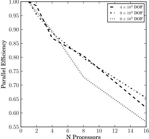
VarGlaS has been developed to take full advantage of the in-nate parallel capabilities of PETSc (Balay et al., 2012) and FEniCS (Logg et al., 2012), on which it is built. All compu-tationally intensive components of the model are compatible with parallel usage, such as the nonlinear solvers, time step-ping, and optimization. VarGlaS exhibits good scaling be-tween 1 and 16 cores, the largest cluster to which the authors have access. Parallel efficiency for a nonlinear solution of the first-order equations over all of Greenland for over a million degrees of freedom is shown in Fig. 2.

2.2.7 Verification with the method of manufactured solutions

We use the method of manufactured solutions (MMS, Salari and Knupp, 2000) to construct analytical solutions to the mo-mentum balance and surface evolution equations in order to determine the extent to which our numerical solutions repro-duce the exact results. This procedure is known as verifica-tion, which ensures that the given equations are being solved correctly and consistently (this is held in contrast to valida-tion, which is the procedure of ensuring that the appropriate equations for a given physical scenario are being solved). The use of MMS in the context of glaciological models has been previously developed by Bueler et al. (2005), with more re-cent results by Sargent and Fastook (2010) and Leng et al. (2013). We adopt a similar approach to these works, but like Leng et al. (2013) and unlike Bueler et al. (2005), we explic-itly forego verifying thermomechanical coupling.

The main idea behind MMS is to select an arbitrary solu-tion, and then construct a source function that produces that solution. To that end, we select the following functions for the components of the ice velocity and free surface:

ˆ

u(x, t )=ud

" 1−

ˆ

S(x, t )−z

ˆ

S(x, t )−B(x)

#

+ub, (34)

ˆ

v(x, t )=0, (35)

ˆ

w(x, t )= −

z

Z

B(x)

_∂uˆ

∂x(x

0

, t )+∂vˆ

∂y(x

0

, t )

dz0, (36)

ˆ

S(x, t )= −xtanα+Amp(1−e−τt₎ ×sin

_2π

L x

sin

_2π

L y

. (37)

Also, we have thatB(x)=S(x, t= ∞)−103,L=104, and Amp=500, which corresponds to the geometric set-up of

0 2 4 6 8 10 12 14 16

N Processors

0.55 0.60 0.65 0.70 0.75 0.80 0.85 0.90 0.95 1.00

Parallel

Efficiency

4×104DOF 9×104DOF 9×105DOF

Fig. 2. Parallel efficiency computed for one complete Newton solve of the first-order equations for meshes with different degrees of freedom. All linear solves were performed using parallel GMRES (generalized minimal residual method) preconditioned with Hypre-AMG.

ISMIP-HOM A (Pattyn et al., 2008). We setud=20 m a−1

andub=10 m a−1

We begin by verifying the computation of the velocity field, which is a pseudo-steady-state calculation; the veloc-ity field’s only dependence on time is through the problem geometry. This implies that we can verify the velocity field independent of time, and for this procedure sett=0.

We seek vector-valued functions F(x, t )and G(x, t )such that the functionsu(x, t )ˆ that we have selected minimize the functional

ˆ

A[ ˆu] =

Z



_2n

n+1η(˙

2_)˙2 _{+ G· ˆu}

d

+

Z

0

ˆ

udiag(G)uˆT d0, (38)

where diag(G)is a diagonal matrix with the components of g on the diagonal. Note that we have eliminated the Lagrange multiplierP from the functional, since uˆ is constructed to be divergence-free. Taking the variation with respect to uˆ

yields the Stokes’ equations with arbitrary forcings within the model domain and at the boundary. Sinceuˆ is analytical, we can invert for F and G. The procedure is the same for finding the forcing functions for the first-order equations, but we use the first-order functional Eq. (6).

While the functions used in the MMS are arbitrary, we note a few features of our selection. We have eliminatedP

One may view the pressure as itself being an arbitrary forc-ing function, and in this case it becomes part of F and G. Also, we have chosenvˆ=0 because it greatly simplifies the analytical source terms, and also because it allows us to carry out an important test of rotational symmetry by swapping the definitions ofuˆandvˆ(and their spatial arguments).

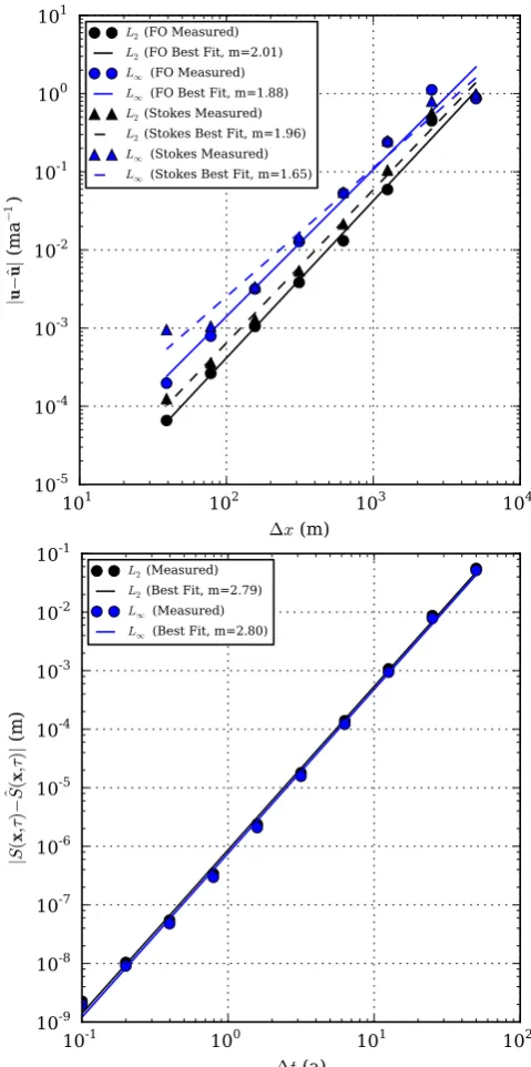
With the analytic forcing functions F and G in hand, as well as their corresponding analytical solutions, we can solve the discrete model over progressively finer meshes and eval-uate whether the error in the numerical solution tends to-wards zero as the discrete domain better approximates the continuum. In practice, computational intensity limits the maximum level of refinement, and it is sufficient to show that a discretization converges towards the analytical solu-tion at close to the theoretical order of accuracy, which for linear finite elements isO(1x2_{)(Salari and Knupp, 2000).}

We solved both of these problems over meshes ranging from

1x=5×103m to1x=40 m, two orders of magnitude. The resulting error profiles are shown in Fig. 3. The slope of the relativeL2norm for both approximations is close tom=2

in logarithmic space, which is the theoretically correct result for linear elements. This confirms that our discretization pro-cedure shows theoretical order of accuracy convergence and thus correctly solves the governing equations for the velocity field.

Verification for our free surface evolution scheme pro-ceeds similarly, except that refinements to the computational domain are carried out both in time and space. We seek a compensatory accumulation fieldc˙, such that the kinematic boundary condition

∂tSˆ+ ˆu∂

ˆ

S ∂x+ ˆv

∂Sˆ

∂y = ˆw+ ˙c (39)

holds for the pre-defined, analytical functions Sˆ and uˆ. Again, it is a simple matter to determine a closed form ex-pression forc˙. We use the same analytical functions as de-fined above, but allowt to vary. To test the convergence of our time-stepping scheme, we progressively refine1t and run the model tot=τ using the compensatory accumulation

˙

cin place ofa˙ in Eq. (14) and evaluate the error in surface elevation at that time. Note that because we are using an ex-plicit time-stepping algorithm, the Courant–Friedrich–Lewy (CFL) condition applies, limiting the minimum cell size that can be used for a given time step. Simultaneously, we require a certain spatial accuracy such that errors in the temporal dis-cretization are not overwhelmed by errors resulting from the spatial discretization. Thus, as we refine the time step, we also refine the spatial resolution such that the Courant num-berC=0.1 for all simulations. This ensures that instability due to a violation of the CFL condition does not occur, and that an appropriately fine spatial resolution is used for a given time step.

We refine between1t=50 a and1t=0.1 a, which corre-spond to spatial resolutions between1x=104m and1x=

10

10

10

10

∆x

(m)

10

10

10

10

10

10

10

|

u

−

ˆ

u

(m

a

−

1

)

L2 (FO Measured) L2 (FO Best Fit, m=2.01) L∞ (FO Measured)

L∞ (FO Best Fit, m=1.88)

L2 (Stokes Measured) L2 (Stokes Best Fit, m=1.96) L∞ (Stokes Measured)

L∞ (Stokes Best Fit, m=1.65)

10

10

10

10

∆t

(a)

10

10

10

10

10

10

10

10

10

|

S

(

x

,τ

)

−

ˆ

S

(

x

,τ

)

|

(m

)

L2 (Measured) L2 (Best Fit, m=2.79) L_∞ (Measured) L_∞ (Best Fit, m=2.80)

Fig. 3. Error between numerical and analytical solutions versus mesh cell size and time step. The slopes of these lines represent the convergence rates of the spatial and temporal discretization methods used by VarGlaS.

20 m. Surface elevation errors are shown in Fig. 3. The theo-retical behaviour of our RK2 algorithm implies a single-step error ofO(1t3_{)and a cumulative error over time ofO(1t}2₎

both theL2andL∞norms. This result shows that our time-stepping scheme possesses theoretical convergence proper-ties, and can be considered verified.

We noted earlier that our choice of velocity fields could be used to test symmetry. We performed both of the above convergence tests for a swapped uˆ andvˆ (with associated swapped coordinatesxandy), and produced convergence re-sults that were identical to machine precision. Thus we con-clude that VarGlaS possesses the appropriate properties of rotational symmetry.

3 Numerical experiments

In order to assess the correctness and efficiency of model, we apply it to a number of well-known ice sheet modelling benchmark experiments, before turning it towards a large-scale data assimilation and prognostic time-stepping simula-tion for the whole Greenland ice sheet.

3.1 ISMIP-HOM

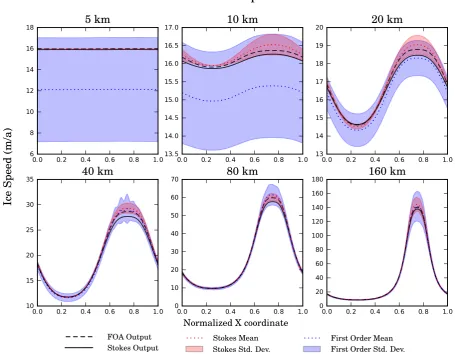
The Ice Sheet Model Intercomparison Project–Higher Order Model (ISMIP-HOM) benchmarks are a widely used test of higher order model capabilities (Pattyn et al., 2008). In order to verify our model performance, we run ISMIP-HOM tests A, B, C, D, and F using both the first-order and Stokes’ equa-tions for the momentum balance. All meshes for the ISMIP-HOM experiments used structured grids with 20 elements in each horizontal dimension, and 10 elements in the vertical dimension, for 4851 degrees of freedom.

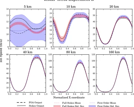
ISMIP-HOM A and ISMIP-HOM B simulate steady ice flow with no basal slip over a sinusoidally varying bed with periodic boundary conditions. B varies from A in that the basal topography does not vary in the transverse direction, whereas in A it does. Note that despite the fact that B is uni-form in one spatial dimension, we still treat it as a three-dimensional problem and use the same discretization and boundary conditions (periodic, namely) as for A. Figures 4 and 5 show the simulated surface velocity for all length scales outlined in the benchmarks.

ISMIP-HOM C and ISMIP-HOM D simulate steady ice flow with sinusoidally varying basal traction over a flat bed with periodic boundary conditions. Again, D varies from C in that only C is transversely varying. Figures 6 and 7 show the simulated surface velocity for all length scales outlined in the benchmark. This experiment specifies thatr=0 in the sliding law.

Experiments A–D were run in serial with a 2.2 GHz laptop computer. Runs using the first-order approximation took ap-proximately 10 s, while runs using the Stokes’ approximation took around 60 s.

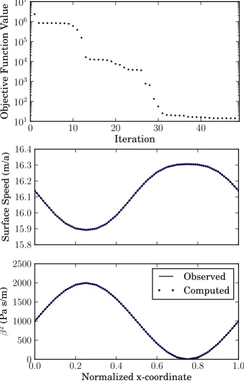
After running the ISMIP-HOM C experiment forward, we have in hand the velocity field predicted by the model for a given basal traction. We used this as an opportunity to

test the inverse capabilities of the model, and to invert for a known basal traction. We performed the inversion using the first-order approximation. Starting from an initial guess of a uniform basal traction of 103Pa a m−1, we allow the inverse model to predict the basal traction field that produces the ve-locity field of the forward model (which we know to be a sinusoid). In assessing misfits, we used the linear cost func-tional Eq. (20), because the velocity scale varies relatively little over the domain. This problem was unregularized, so

α=0. Figure 8 shows both the rate of convergence as well as the “observed” and modelled basal tractions and surface velocities along the L₄ transect of the ISMIP-HOM model domain using the results for the first-order approximation at theL= 10 km length scale. Results for other length scales are similar.

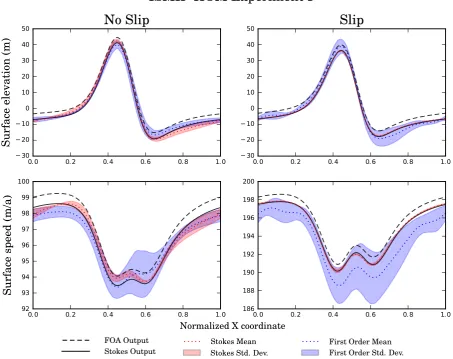
ISMIP-HOM F simulates unsteady ice flow over a Gaus-sian bump with periodic boundary conditions under slip and non-slip conditions, and evaluates the surface geometry and velocity as they relax to steady state. Experiment F also man-dates a linear rheology, son=1. Figure 9 shows the simu-lated surface velocities and elevations for the slip and non-slip cases, using a time step of1t=1 a. These experiments were run on a 4-core machine with 8 GB of memory and 2.2 GHz per processor. Using the first-order approximation, the 500 a run took approximately 50 min. Using the Stokes’ approximation, the run took 5.5 h.

3.2 EISMINT II

The European Ice Sheet Model INTercomparison II (EIS-MINT II) benchmarks are an older set of benchmarks than ISMIP-HOM, and were designed for use with models em-ploying the shallow ice approximation (Payne et al., 2000). While ISMIP-HOM generally tests the accuracy of the mo-mentum balance scheme over varying length scales, the EISMINT experiments are more focused towards assessing the time-dependent mass and energy balances. EISMINT II stresses the dynamic evolution of the system and provides a test for the long-term stability of our time-stepping scheme. We know of no other higher order model operating on an unstructured grid that has demonstrated a capacity to run for-ward on such timescales.

0.0 0.2 0.4 0.6 0.8 1.0 10

12 14 16 18 20 22

24

5 km

0.0 0.2 0.4 0.6 0.8 1.0

10 15 20 25 30

35

10 km

0.0 0.2 0.4 0.6 0.8 1.0

5 10 15 20 25 30 35 40

45

20 km

0.0 0.2 0.4 0.6 0.8 1.0

0 10 20 30 40 50 60

70

40 km

0.0 0.2 0.4 0.6 0.8 1.0

0 20 40 60 80

100

80 km

0.0 0.2 0.4 0.6 0.8 1.0

0 20 40 60 80 100

120

160 km

ISMIP-HOM Experiment A

Normalized X coordinate

Ic

e

Sp

eed

(m

/a

)

FOA Output

Stokes Output Stokes Std. Dev.Stokes Mean

First Order Mean First Order Std. Dev.

Fig. 4. ISMIP-HOM A performed using first-order and Stokes’ approximations.

the ice sheet were 3647 m and 255.4 K respectively. These are important metrics for intercomparison performance, and lie near the benchmark means of 3688 m and 255.605 K.

EISMINT II F is identical to experiment A, except that im-posed surface temperatures are 15◦C colder throughout the model domain. The results of this experiment are similar to those of experiment A, albeit with a thicker ice sheet, and a slightly different basal temperature profile. The resulting thickness and basal temperature fields are given in Fig. 10 An interesting difference between the resulting temperature field here and that documented in the EISMINT II paper is that VarGlaS does not predict the breakdown in radial symmetry that occurred in all of the finite difference models of the inter-comparison. We suspect that this is due to VarGlaS using an unstructured grid, which alleviates some of symptoms of grid dependency seen in the original experiment. This hypothesis is supported by the work of Saito et al. (2006), who provides evidence that suggests that the “spoking” phenomenon seen in Payne et al. (2000) is numerical in origin. It could be the

case that using an unstructured grid removes the grid-induced pathways that allow these spokes to form.

3.3 Greenland

We applied VarGlaS to a large-scale problem in glaciology, namely the transient simulation of the Greenland ice sheet. The strategy in so doing was to initialize the model us-ing measured present-day geometry, apply data assimilation tools to obtain an initial estimate of the basal traction field, and then allow Greenland’s geometry, velocity, and temper-ature to evolve over 500 yr. We performed all simulations of Greenland using the first-order approximation for the mo-mentum balance (see Eq. 6).

3.3.1 Data

0.0 0.2 0.4 0.6 0.8 1.0 8

9 10 11 12 13

14

5 km

0.0 0.2 0.4 0.6 0.8 1.0 8

10 12 14 16 18 20 22 24

26

10 km

0.0 0.2 0.4 0.6 0.8 1.0 0

10 20 30 40 50

60

20 km

0.0 0.2 0.4 0.6 0.8 1.0 0

10 20 30 40 50 60 70

80

40 km

0.0 0.2 0.4 0.6 0.8 1.0 0

20 40 60 80 100

120

80 km

0.0 0.2 0.4 0.6 0.8 1.0 0

20 40 60 80 100

120

160 km

ISMIP-HOM Experiment B

Normalized X coordinate

Ic

e

Sp

eed

(m

/a

)

FOA Output

Stokes Output Full Stokes MeanFull Stokes Std. Dev.

First Order Mean First Order Std. Dev.

Fig. 5. ISMIP-HOM B performed using first-order and Stokes’ approximations.

Fausto et al. (2009), basal heat fluxes from Shapiro and Ritz-woller (2004), and surface mass balances from Ettema et al. (2009). We used InSAR-derived 2007–2008 average surface velocities from Joughin et al. (2010) for a surface velocity target. The Joughin data set is incomplete. The gaps were filled with balance velocities, with gradients between the two reduced by systematically exploring the uncertainties in the accumulation rate. Specifically, we used a steepest descent algorithm to minimize the misfit between the edges of the InSAR velocities and the corresponding balance velocities by varying the surface mass balance subject to the constraint that it remains within its reported point-wise error bounds. 3.3.2 A mesh for Greenland

The boundary of Greenland was digitized using the 1 m con-tour of the Bamber et al. (2001) thickness data. We created an initial two-dimensional (map plane) mesh by imposing a 2 km element size at the margins, grading to a variable but much coarser resolution at the centre of the ice sheet. This

0.0 0.2 0.4 0.6 0.8 1.0 6

8 10 12 14 16

18

5 km

0.0 0.2 0.4 0.6 0.8 1.0 13.5

14.0 14.5 15.0 15.5 16.0 16.5

17.0

10 km

0.0 0.2 0.4 0.6 0.8 1.0 13

14 15 16 17 18 19

20

20 km

0.0 0.2 0.4 0.6 0.8 1.0 10

15 20 25 30

35

40 km

0.0 0.2 0.4 0.6 0.8 1.0 0

10 20 30 40 50 60

70

80 km

0.0 0.2 0.4 0.6 0.8 1.0 0

20 40 60 80 100 120 140 160

180

160 km

ISMIP-HOM Experiment C

Normalized X coordinate

Ic

e

Sp

eed

(m

/a

)

FOA Output

Stokes Output Stokes Mean_{Stokes Std. Dev.} First Order MeanFirst Order Std. Dev.

Fig. 6. ISMIP-HOM C performed using first-order and Stokes’ approximations.

this mesh is variable, but grades from 500 m at the edges of the domain to approximately 100 km over the interior of the ice sheet. We used a coarser mesh with 4×104nodes for our transient run, corresponding to 8×104degrees of freedom for the first-order model. This corresponds to a minimum horizontal resolution of 5000 m up to approximately 100 km in the interior.

3.3.3 Data assimilation

We calculated a basal traction field using the techniques of Sect. 2.2.3. We begin by calculating steady-state velocity and enthalpy fields for an arbitrary basal traction (with an initial guess of 4 Pa a m−2), withr equal to unity (which implies that basal traction is linearly scaled by thickness; this effec-tively eliminates the dependence of sliding speed on normal force, and eliminates the covariance betweenβ2andh). With this initial state in hand, we ran the BFGS algorithm using a fixed viscosity (and an incomplete adjoint) for the first 10 iterations, before switching to a full adjoint. The selection

0.0 0.2 0.4 0.6 0.8 1.0 4

6 8 10 12 14 16 18

20

5 km

0.0 0.2 0.4 0.6 0.8 1.0 12

13 14 15 16 17 18

19

10 km

0.0 0.2 0.4 0.6 0.8 1.0 10

12 14 16 18 20 22 24

26

20 km

0.0 0.2 0.4 0.6 0.8 1.0 10

15 20 25 30 35 40

45

40 km

0.0 0.2 0.4 0.6 0.8 1.0 0

20 40 60 80 100

120

80 km

0.0 0.2 0.4 0.6 0.8 1.0 0

50 100 150 200 250

300

160 km

ISMIP-HOM Experiment D

Normalized X coordinate

Ic

e

Sp

eed

(m

/a

)

FOA Output

Stokes Output Full Stokes MeanFull Stokes Std. Dev.

First Order Mean First Order Std. Dev.

Fig. 7. ISMIP-HOM D performed using first-order and Stokes’ approximations.

glacier in eastern Greenland. The modelled velocity field matches the observed field closely, and the RMS error for the whole ice sheet is approximately 36 m a−1. For outlet glaciers like Kangerdlugssuaq, we see that surface velocity can be explained by spatially variable basal traction field composed of both low traction streaming features, and sticky pinning points that slow flow. Basal temperature is also re-lated to basal traction, where fast sliding is associated with a melted bed.

3.3.4 Prognostic run

After performing the data assimilation procedure outlined above, we allowed the ice sheet to evolve through time for 500 yr under the C1 (constant climate) SeaRISE experiment, with a time step of 0.1 a. On a 16-core machine with 400 GB of memory and 2.9 GHz per processor, this run took 27 h. The present-day measured surface elevation of Greenland is not in a steady state with respect to the basal topography and the inverted velocity field, which is unsurprising given

the errors associated with the basal topography, the surface velocity field, and the approximations made by the model physics. Because of this mismatch, large transient signals propagate through the system at the beginning of the run. We monitored the size of these transients as the L∞ norm of the∂tS field, given by Fig. 14. Note the exponential de-cay rate; this gives some estimate of how much relaxation a model requires in order to eliminate transients. Results from Pritchard et al. (2009) show that the average∂tSof the

Greenland ice sheet (GrIS) is−0.84 ma. An ice sheet model should have relaxed to around this level before any conclu-sions should be drawn from additional forcing being applied to it. For VarGlaS, with the specified data inputs, this pro-cess takes about 100 a. We also monitored the mass of the entire ice sheet throughout time. After the initial transient pe-riod of ice increase, we found an annual average total ice de-crease of 10−3% a−1(2.63×103Gt a−1), which is in order-of-magnitude agreement with the GRACE-derived ice loss of approximately 6×10−3_{% a}−1_(17.7×103_{Gt a−1) (Baur}

0 10 20 30 40

Iteration

101

102

103

104

105

106

107

Objective

Function

Value

15.8 15.9 16.0 16.1 16.2 16.3 16.4

Surface

Speed

(m/a)

0.0 0.2 0.4 0.6 0.8 1.0

Normalized x-coordinate

0 500 1000 1500 2000 2500

β

2(P

a

s/m)

Observed Computed

Fig. 8. Convergence profile and modelled basal traction and velocity from inverting ISMIP-HOM C using the first-order approximation. RMS between observed and modelled velocities is 5×10−3m a−1.

of the basal temperature field changes relatively little over 500 yr. Although relative to the magnitude of their initial val-ues, thickness and velocity also change relatively little; they show an interesting qualitative pattern that explains the mass loss of Fig. 14. We see that over time the combination of surface mass balance and basal traction tends towards thin-ning the interior of the ice sheet, while thickethin-ning the edges. This change is most notable where ice stream development is apparent, such as Jakobshavn and Kangerdlugssuaq, as well as the outlet glaciers of the southern GrIS. This increase in thickness generates a steeper ice surface at outlets, elevating the flux through the lateral boundaries. Since ice loss due to surface mass balance is constant (because surface mass bal-ance itself is constant), the change in total mass for the GrIS is driven wholly by this increased boundary flux. This pattern of thickness and velocity evolution is also seen in compara-ble simulations of the GrIS, such as in Seddik et al. (2012)

and Larour et al. (2012). This pattern is problematic, because it suggests an opposite redistribution of mass from that mea-sured through remote sensing (Pritchard et al., 2009; Baur et al., 2009). More work is needed to determine if this mass loss rate is believable.

4 Discussion

VarGlaS performs well in a number of standard benchmark-ing experiments and can also simulate the evolution of the GrIS using higher order physics and thermomechanical cou-pling, as well as an advanced treatment of time evolution.

For the diagnostic and isothermal ISMIP-HOM bench-mark experiments, both VarGlaS first-order and Stokes’ solvers perform well with respect to existing benchmark re-sults, with our first-order solver generally predicting values close the the Stokes’ mean, and our Stokes’ solver generally predicting velocities slightly slower than those reported by the benchmark. Our data assimilation procedure is able to re-produce effectively these simple imposed basal traction fields through model inversion. Both first-order and Stokes’ solvers performed well on the prognostic ISMIP-HOM F, yielding velocity and surface elevation fields that are in good agree-ment with other models. Results for the EISMINT II exper-iments are similar, with model results comparing favourably to mean values from the original publication. Also, thickness and temperature fields compare well with the results of Pat-tyn (2003) and Saito et al. (2003), who also applied higher order models to these experiments. Note that this is the first time that the EISMINT II experiments have been performed with a higher order finite element model using an unstruc-tured mesh.

VarGlaS’ behaviour over the entire Greenland ice sheet echoes what has been determined by various investigators in the past, which is that after the relaxation of a strong transient signal derived from the incompatibility of flawed basal topography, surface velocities, and surface mass bal-ance data, the ice sheet seems to be losing mass on the order of 10−3% a−1, which is in agreement with contemporary es-timates, although the qualitative distribution of this mass loss is not entirely believable. Performing simulations of this tem-poral length and at this spatial resolution has only been made possible by a combination of advances in ice sheet modelling technology, namely variable spatial resolution, data assimila-tion, and parallelism.

0.0 0.2 0.4 0.6 0.8 1.0

−30

−20

−10 0 10 20 30 40 50

Su

rf

ac

e

el

ev

at

ion

(m

)

No Slip

0.0 0.2 0.4 0.6 0.8 1.0

92 93 94 95 96 97 98 99 100

Su

rf

ac

e

sp

eed

(m/a

)

0.0 0.2 0.4 0.6 0.8 1.0

−30

−20

−10 0 10 20 30 40

50

Slip

0.0 0.2 0.4 0.6 0.8 1.0

186 188 190 192 194 196 198 200

ISMIP-HOM Experiment F

Normalized X coordinate

FOA Output

Stokes Output Stokes MeanStokes Std. Dev.

First Order Mean First Order Std. Dev.

Fig. 9. ISMIP-HOM F performed using first-order and Stokes’ approximations.

the calculation of a starting enthalpy field, which would be of a much lower quality without incorporating the very sig-nificant heat source due to friction at the bed.

We employed an anisotropically refined, variable resolu-tion mesh in order to minimize superfluous degrees of free-dom in slowly varying regions of the ice sheet while main-taining detailed solutions in regions of large velocity gradi-ents. Although variable resolution modelling is not impos-sible with finite differences (Colella et al., 2000; Cornford et al., 2013), it is applicable to finite elements in a straight-forward way.

Parallelism was another critical component in modelling the whole Greenland ice sheet. The number of degrees of freedom is simply too large for one processor to handle in a reasonable amount of time. We found that we retained bet-ter than 50 % parallel efficiency for nearly 1 million degrees of freedom and 16 processors, using an iterative solver. This corresponds to a speed-up of around a factor of 10. With the increasing availability of large computers with many proces-sors, the benefit of incorporating parallelism into model

de-sign is clear. Diagnostic modelling of very large ice sheets at resolutions similar to those of contemporary data products is possible with even modest computers. For example, in this paper, we perform data assimilation over the entire Green-land ice sheet at the horizontal scale of a few ice thicknesses using 16 cores in 3.5 h, which we believe is reasonable. For prognostic simulations with this same resolution, particularly past the century timescale, larger clusters are necessary. For example, for prognostic simulations with a 0.1 a time step and the same spatial resolution as the data assimilation exer-cise, using the same machine, we can simulate one year of model time in one day of real time. This is not practical. For-tunately, there now exist many clusters with many thousands of processors, and this type of computing power is becoming more available, such that, with sufficient parallel efficiency, solutions of problems at long timescales and at high spatial and temporal resolution are plausible.

Fig. 10. Thickness and basal temperature fields for EISMINT II A and F at 200 ka.

0 50 100 150 200

Iteration

1011

1012

Objective

Function

Value

Fig. 11. Convergence rate of L BFGS B algorithm for surface ve-locity assimilation over the GrIS, using basal traction as a control variable. Vertical lines are where the enthalpy equations were recal-culated

Fig. 12. Modelled and measured surface velocities, basal traction, and basal temperature of the GIS after assimilation of surface ve-locity. RMS velocity mismatch is 36 m a−1.

calving would also be necessary to simulate accurately the grounding line dynamics. VarGlaS currently does not have the capacity to move the lateral bounds of its computational domain. Leaving the thickness at the lateral boundaries fixed is equivalent to making the assumption that any flux through the boundary in excess of the present rate calves immedi-ately, or is otherwise removed from the ice sheet, and that the height of that boundary is fixed. This may be valid for continental scale model runs where the geometry of the ice sheet is not expected to adjust dramatically. This treatment is certainly insufficient for regional-scale experiments such as modelling the response of inland glaciers to ice shelf col-lapse.

Data assimilation is an essential part of correctly mod-elling ice surface velocities. Without using inverse methods to estimate the value of the basal traction field, the observed pattern of surface velocities is not well reproduced, and the

Fig. 13. Modelled and measured surface velocities, basal traction, and basal temperature of Kangerdlugssuaq glacier in eastern Green-land after assimilation of surface velocity.

100 101 102 103

k

∂

S k _∂t

L∞

(ma

−

1 )

0 100 200 300 400 500

time (a) 0.996

0.997 0.998 0.999 1.000 1.001

M(t)/M

0

26.22 26.24 26.26 26.28 26.30 26.32 26.34

M(t)

(gt

×

10

5)

Fig. 14. TheL∞norm of the surface elevation change field and the total ice mass over a 500-year model run.

to subglacial water routing and pressure. Under changing climate scenarios, delivery of water to the bed may change dramatically, and this could fundamentally alter basal trac-tion. Similarly, changes in ice sheet geometry are expected to change the pattern of basal traction through changes in ice overburden pressure as well as surface-elevation-forced wa-ter input. For a non-trivial portion of the ice sheet, basal trac-tion is a zero-order control on all model physics. Long-term prognostic simulations involving major changes in climate or ice sheet geometry must include a mechanism for estimating changes in basal traction.

With the major increases in efficiency gained from par-allelism and anisotropic mesh refinement, it is tempting to model on increasingly detailed meshes, simply due the phi-losophy that this will give us more detailed and thus more meaningful results. In an ideal scenario, the data from which we draw our surface elevations, bed elevations, surface ve-locities, and surface mass balances are effectively error-free and at spatial resolutions much finer than the grids on which we model. This may have been the case in the past, when the errors derived from using the shallow ice approximation were larger than those inherent in data, and low spatial res-olution grids could average from a number of data points falling within a given pixel. It is certainly not the case now. It is simple to generate meshes with a horizontal resolution of near an ice thickness, but it is not simple to determine how to interpolate accurately from 5 km thickness data down to this resolution. Nevertheless, in some heavily studied

re-Fig. 15. Velocity, surface elevation, and basal temperature change through a 500-year simulation of the Greenland Ice Sheet.

gions of the GrIS, data at thickness-scale horizontal resolu-tion exist (e.g. Jakobshavn, Russell–Isunnguata Sermia), and these should be incorporated when possible. For the future, we intend to incorporate error metrics over all of VarGlaS’s input data into our mesh generation procedure, in order to avoid obtaining spurious results and using unnecessary com-putational resources as a result of over-resolving in regions where the data do not have a commensurate level of detail.

5 Conclusions

efficient solvers, and demonstrably scalable parallelism. Var-GlaS eschews the common stress balance formulation of ice flow physics in favour of formulation as the problem of min-imizing a scalar variational principle representing the con-version of gravitational potential energy into heat under the constraint of incompressibility. We use an enthalpy formula-tion for the energy balance equaformula-tions, exchanging the tem-perature equation’s contact problem for additional nonlinear-ity. VarGlaS treats conservation of mass using the kinematic boundary condition.

We applied VarGlaS to the ISMIP-HOM benchmarks for higher order models, as well as several of the EISMINT II experiments. VarGlaS performed well in all of these bench-marks, proving that it correctly solves the field equations. Additionally, we applied VarGlaS’s data assimilation to one of the benchmark experiments, showing that it can recover a simple basal traction field from an observed