Direct method for Solving Nonlinear Variational Problems
by Using Hermite Wavelets
Zina K. Alabacy*
Asmaa A. Abdulrehman**
Lemia A. Hadi **
Received 16, June, 2014 Accepted 14, September, 2014
This work is licensed under a Creative Commons Attribution-NonCommercial-NoDerivatives 4.0 International Licens
Abstract:
In this work, we first construct Hermite wavelets on the interval [0,1) with it’s product, Operational matrix of integration is derived, and used it for solving nonlinear Variational problems with reduced it to a system of algebric equations and aid of direct method. Finally, some examples are given to illustrate the efficiency and performance of presented method.
Key words: Hermite wavelets, Operational Matrix of integration, Matrix of product,
Nonlinear Variational problems.
Introduction:
Wavelets theory is relatively new in mathematical researches [1], wavelets constitute a family of functions constructed from dilation and traslation of a single function called the mother wavelet [2]. When the dilation parameter a and the translation parameter b vary continuously we have the following family of constituous wavelets:
( ) | | [ ]
… (1)
An efficien algorthithm based on Chebyshev wavelets as simplest wavelets approach for numerical solution of many problems such that integrel equations, Variational problems, and diffrentional equations is given in [3-5].
Other wavelets families like Legendre wavelets [6], Sine and Cosine wavelets [7], Harr wavelets [8], are used to solve integral equation first and second kind and are used in solving many kinds problems.
Properties of the Hermite
Wavelets:-
Hermite
wavelets, ( ) ( ) involve four arguments, , k is assumed any positive integer, m is the degree of the Hermite polynomials and t independent variable in [0,1].( )
{ ( ) [ ] … (2)
where
√ … (3)
m=0,1,2,...,M-
( ) ( ) ( )
… (4)
( ) ( )
Starting with
Orthgonality of Hermite polynomials
∫ ( ) ( )
{
√ …(5)
So that the Hermite polynomials are mutually orthogonal with respect to the weight function or density function
and if m=n we can normalize the
Hermite polynomial so as to obtain an orthonormals set.
Function approxemation: Afunction f(t) defined over [0,1) may be expanded as
A function f(t) defined over [0,1) as:
. ( ) ∑ ∑ ( ) …(6)
where
( ( ) ( )) ∫ ( ) ( ) ( )
in which ( ) denoted the inner product in [ ]
If the infinite series in equation(6) is truncated, then it can be written as:
( )
∑ ∑ ( )
( )
…(7)
where F and ( ) are matrices given by:
[ ]
( ) =
[ ( ) ( ) ( ) ( ) ( ) ( ) ( )]
[ ( ) ( ) ]
… (8)
Operation Matrix of Integration:
In this section we will know the operational matrix P of integration. the six basis functions when M=3, k=1 are given by:
( ) √ √
( ) √ √ ( )
( ) √ √ ( ) }
… (9)
( ) √ √
( ) √ √ ( )
( ) √ √ ( ) }
…(10)
By integrating the above six functions from 0 to t and using eq(6), we obtain:
∫ ( ) ( ) ( )
( ) ( ) ( ) ( )
∫ ( ) ( ) ( )
( ) ( ) ∫ ( ) ( ) ( )
( ) ( ) ∫ ( ) ( ) ( )
( ) ( )
∫ ( ) ( ) ( )
( ) ( )
∫ ( ) ( ) ( )
P=[
] since
Q=
[
( ) ( ) ]
, S=
[
( )
( ) ]
and O= [
]
Operation matrix of product and there properties:
Product Operational matrix, which is important for solving our problem and many other problems such that Volterra integral equation , Fredholm integral equation and Integro defferential eqs [5-8] .
Let ( ) ( ) ̃ ̃ ( ) …(11) where ̃ is ( ) ( ) product Operational matrix for k=1,2,… n=1,2,…,
m=0,1,2,…(M-1)
where √
√ ( )
Thus we get
( ) ( )
[
]
Expanding each product by wavelet basis we have matrix D
√
[
( )
( ) ]
By using the vector C, the ̃ is
̃ √ [ ̃
̃ ] ̃
√ [
( )
]
and integrating matrix D from 0 to 1 we obtained new matrix denoted by matrix R
where
∫ ( ) ( ) (12)
if we take k=0, M=3 we obtain
[
]
Problem Statement:
In large number of problems a
rising in analysis, mechanics and geometry it is necessary to determine the maximal and minimal of acertain functional. Such problems are called Variational problems .Consider the following Variational problem
[ ( )]
∫ ( ( ) ̇( ) ( ) … (13)
with ( ) ̇( ) ( )
This problem with moving boundary conditions, and find the extremum of eq(13), above problem is reduced by using our method in to a set of algebric equations by following procetuer.
( ) ( ) ( )
( ) ( )
( ) ( )
( )
( )
( )
Numerical examples:
Example(1)
[ ( )] ∫ ̇ ( ) ̇( ) … (14)
with boundary conditions:
( )
( ) unspecified (15)
We solve this problem by using Hermite wavelets. First we assume
̇( ) ( ) … (16) ( ) …(17)
Substituting (16),(17) in (14) and we used matrix R then eq(14) becomes
According to transversality condition, we have:
̇| ̇( )
By using (16) ̇( ) ( )
Let ( ( ) )
( )
(18)
For M=3 and k=1, we obtain:
[ ]
Thus
[
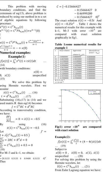
] The exact solution ̇( ) And ( ) . Table 1 shows the numerical results for this example with k=1, M=3 with error =10-8 are compared with exact solution graphically in fig1.
Table 1:some numerical results for example 1
x Exact solution
Approximat
solution ( )
| |
0 0.00000000 0.00000000 0.00000000
0.1 -0.00250000 -0.00250000 0.00000000 0.2 -0.01000000 -0.01000000 0.00000000 0.3 -0.02250000 -0.02250000 0.00000000 0.4 -0.04000000 -0.04000000 0.00000000 0.5 -0.06250000 -0.06250000 0.00000000 0.6 -0.09000000 -0.09000000 0.00000000 0.7 -0.12250000 -0.12250000 0.00000000 0.8 -0.16000000 -0.16000000 0.00000000 0.9 -0.20250000 -0.20250000 0.00000000 1 -0.25000000 -0.25000000 0.00000000
=
=
Fig(1) error =10-8 are compared
with exact solution
Example(2):
[ ( )] ∫ ̈ ( ) ( ) ̇( ) … (19)
Subject to
( ) ̇( ) ( ) ̇( ) unspecified … (20)
For solving this problem by using the Hermite wavelets, let:
⃛( ) ( ) …(21)
From Euler Lagrang equation we have:
0 0.1 0.2 0.3 0.4 0.5 0.6 0.7 0.8 0.9 1 -0.25
-0.2 -0.15 -0.1 -0.05 0
̇ ̈| ( ) ⃛( )| ⃛( ) , ̈|
̈( ) (22)
̈( ) ( ) ̈( ) (23) ̈( ) ∫ ( ) ̈( ) Let ∫ ( ) [ ] ̈( ) ( ) (24) Then F= [ ] Also ̇( ) ( ) ( ) (25) Let ( )
Similarly example(1) is written J For M=3 and k=1 we obtain: [ √
√ √ √
√
√ ] , and
[
]
Approximate solution will be achieved
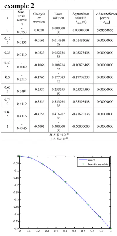
( ) ( ) which is the exact solution.
Table (2), the values of x(t) using the Hermite wavelets, Chebyshev wavelets and Sine-Cosine , are compared with exact solution. The Hermite wavelets with error =10-8 graphically in fig(2).
Table 2:some numerical results for example 2 x Sine-cosin wavele ts Chebysh ev wavelets Exact solution Approximat solution ( ) | | 0
-0.0253 0.0020
0.000000
00 0.00000000 0.00000000 0.12
5
-0.0155 -0.0161 -0.014360
68
-0.01436068 0.00000000
0.25
-0.0119 -0.0523 -0.052734
38
-0.05273438 0.00000000
0.37 5
-0.1069 -0.1066 -0.108764
65
-0.10876465 0.00000000
0.5
-0.2513 -0.1765 -0.177083
33
-0.17708333 0.00000000
0.62 5
-0.2494 -0.2537 -0.253295
90
-0.25329590 0.00000000
0.75 0
-0.4119 -0.3335 -0.333984
38
-0.33398438 0.00000000
0.87 5
-0.4116 -0.4158 -0.416707
36
-0.41670736 0.00000000
1
-0.4946 -0.5001 -0.500000
00
-0.50000000 0.00000000
=
=
Fig(2) The Hermite wavelets with
error =10-8
Conclusion:
In
this work, nonlinear Variational problems have solved by using Hermite wavelets in direct method. Comparison of the approximate solutions and the exact solution shows that the proposed method is very efficient tool.References:
1. Shihab. S. N. and Abdalelah. A. 2012. Numerical Solution of Calculus of Variations by using the Second Chebyshev Wavelets, Eng. & Tech. Journal. 30(18): 3219-3229.
2. Arsalani.M. and Vali.M.A. 2011. Numerical solution of Nonlinear Variational Problems with Moving Boundary Conditions by Using Chebyshev Wavelets, App Math Scie. 5(20):947-964.
3. Abdalelah. A. 2014. Numerical solution of Optimal problems using new third kind Chebyshev Wavelets Operational matrix of integration, Eng. & Tec. Journal. 32(1):145-156. 4. Hosseini. S.Gh.2011. Anew Operational Matrix of derivative for Chbysheve wavelets and Applicationas in solving diffrential equations with non analytic Solution, Appl. Math. Scien. 5(51):2537-2548.
5. Aminsadrabab.S. 2011. Numerical Solution of Itegral equations with Legendre Basis, Int. J. Contemp. Math. Scie. 6(23):1131-1135.
6. Rahbar.S. 2007. Anumerical Solution to the linear and nonlinear Fredholm integral equations using Legendre wavelets functions, PAMM.Proc.Appl.Math.Mech. 7(10):2020149-2020150.
7. Kajani. M. and hasem. M. 2006. Numerical Solution of Linear Integro Differential Equation by Using Sine-Cosine Wavelets, Appl. Math. Comput.1(8): 569-574. 8. Shihab. S. N. and Mohammed. A.
2012. An Efficient Algorithm for nthOrder Integro- Differential Equations Using New Haar Wavelets Matrix Designation, International Journal of Emerging. Technologies in Computational and Applied Sciences (IJETCAS). 12(209): 32-35.
طخ ريغلا رياغتلا لئاسم لحل ةرشابملا ةقيرطلا
ةيجوملا تمره مادختساب ةي
يسابعلا ليلخ ةنيز
*نمحرلا دبع هللاا دبع ءامسأ
*يداه ريملاا دبع ءايمل
نكتلا ةعماجلا ,مظنلاو ةرطيسلا ةسدنه مسق و
ايجول
نكتلا ةععماجلا ,ةيقيبطتلا مولعلا مسق* و
ايجول
:ةصلاخلا
( ةرتفلا يف ةيجوملا تمره لاود ءانب لاوا مت ,لمعلا اذه يف 1
, 4 ةفوفصمو لاودلا هذه برض عم ]
اهداعبا نوكت يتلا تايلمعلا
k
M 2
k
M× 2 ةيطخ ريغلا رياغتلا لئاسم لح يف تافوفصملا هذه مادختسا متو ,
نلا يفو .ةيطخلا ةيربجلا تلاداعملا نم ماظنل اهليوحت عم ةرشابملا ةقيرطلاب مت يتلا ةاطعملا ةلثملأا ضعب ةياه
. ءافكلأا ةقيرطلا اهناب اهللاخ نم انلصوت يتلاو ةضورعملا ةقيرطلاب اهلح
:ةيحاتفملا تاملكلا