Fast and simple model for atmospheric radiative transfer

(1)

Atmos. Meas. Tech., 3, 1129–1141, 2010 www.atmos-meas-tech.net/3/1129/2010/ doi:10.5194/amt-3-1129-2010

Atmospheric

Measurement

Techniques

Fast and simple model for atmospheric radiative transfer

F. C. Seidel1, A. A. Kokhanovsky2, and M. E. Schaepman1

1_{Remote Sensing Laboratories, University of Zurich, Winterthurerstr. 190, 8057 Zurich, Switzerland} 2_{Institute of Environmental Physics, University of Bremen, O. Hahn Allee 1, 28334 Bremen, Germany} Received: 2 May 2010 – Published in Atmos. Meas. Tech. Discuss.: 18 May 2010

Revised: 6 August 2010 – Accepted: 16 August 2010 – Published: 25 August 2010

Abstract. Radiative transfer models (RTMs) are of utmost importance for quantitative remote sensing, especially for compensating atmospheric perturbation. A persistent trade-off exists between approaches that prefer accuracy at the cost of computational complexity, versus those favouring simplic-ity at the cost of reduced accuracy. We propose an approach in the latter category, using analytical equations, parameter-izations and a correction factor to efficiently estimate the effect of molecular multiple scattering. We discuss the ap-proximations together with an analysis of the resulting per-formance and accuracy. The proposed Simple Model for At-mospheric Radiative Transfer (SMART) decreases the calcu-lation time by a factor of more than 25 in comparison to the benchmark RTM 6S on the same infrastructure. The relative difference between SMART and 6S is about 5% for space-borne and about 10% for airspace-borne computations of the atmo-spheric reflectance function. The combination of a large solar zenith angle (SZA) with high aerosol optical depth (AOD) at low wavelengths lead to relative differences of up to 15%. SMART can be used to simulate the hemispherical conical reflectance factor (HCRF) for spaceborne and airborne sen-sors, as well as for the retrieval of columnar AOD.

1 Introduction

The terrestrial atmosphere attenuates the propagation of the solar radiation down to the Earth’s surface and back up to a sensor. The scattering and absorption processes in-volved disturb the retrieval of quantitative information on surface properties. Radiative transfer models (RTMs) and their inversions are commonly used to correct for such ef-fects on the propagation of light. Well-known RTMs are

Correspondence to: F. C. Seidel

(felix.seidel@geo.uzh.ch)

6S (Second Simulation of a Satellite Signal in the Solar Spectrum) (Vermote et al., 1997), SCIATRAN (Rozanov et al., 2005), SHARM (Muldashev et al., 1999; Lyapustin, 2005), RT3 (Evans and Stephens, 1991), RTMOM (Gov-aerts, 2006), RAY (Zege and Chaikovskaya, 1996), STAR (Ruggaber et al., 1994) and Pstar2 (Nakajima and Tanaka, 1986; Ota et al., 2010), as well as DISORT (Stamnes et al., 1988), which is used in MODTRAN (Berk et al., 1989), STREAMER (Key and Schweiger, 1998) and SBDART (Ricchiazzi et al., 1998). These accurate but complex RTMs are frequently run in a forward mode, generating look-up tables (LUTs), which are later used during the inversion process for atmospheric compensation (Gao et al., 2009) or aerosol retrieval (Kokhanovsky, 2008; Kokhanovsky and Leeuw, 2009; Kokhanovsky et al., 2010), for instance. There are also a series of highly accurate, but computationally in-tensive Monte Carlo photon transport codes available. How-ever, the best accuracy may not be always desirable for a RTM. Approximative equations have been developed be-fore computers were widely available (Hammad and Chap-man, 1939; Sobolev, 1972). With regard to the growing size and frequency of remote sensing datasets, approxima-tive and computationally fast RTMs are becoming relevant again (Kokhanovsky, 2006; Katsev et al., 2010; Carrer et al., 2010). In particular, RTMs of the vegetation canopy and fur-ther algorithms that exploit data from imaging spectroscopy instruments (Itten et al., 2008) often rely on fast atmospheric RTM calculations.

In this context, we propose the fast Simple Model for Atmospheric Radiative Transfer (SMART). It is based on approximative analytical equations and parameterizations, which represent an favourable balance between speed and accuracy. We consider minimised complexity and computa-tional speed as important assets for downstream applications and define an acceptable uncertainty range of up to 5–10% for the modelled reflectance factor at the sensor level, under typical mid-latitude remote sensing conditions. SMART can

(2)

therefore be used as a physical model, maintaining a cause-and-effect relationship in atmospheric radiative transfer. In-stead of depending on the classic LUT approach, it permits parameter retrieval in near-real-time. This enables the rapid assessment of regional data requiring exhaustive correction, such as imaging spectrometer data. Furthermore, it supports the straightforward inversion of aerosol optical depth (AOD; τ_λaer) by implementing radiative transfer equations as a func-tion of τ_λaer. The theoretical feasibility for the retrieval of aerosols in terms of the sensor performance was shown in Seidel et al. (2008) for the APEX instrument (Itten et al., 2008).

In this paper, we describe the two-layer atmospheric model with the implementation of approximative radiative transfer equations in both layers and at the Earth’s surface. We then assess the accuracy and performance of SMART in compar-ison with 6S.

2 SMART – a simple model for atmospheric radiative transfer

A remote sensing instrument measures the spectral radiance as a function of the spectral atmospheric properties and the illumination/observation geometry Lλ(τλ,Pλ(2),ωλ;µ0,µ,φ−φ0), where τλ is the optical depth,Pλ(2)is the phase function at the scattering angle2, ωλis the single scattering albedo,µ0=cosθ0,µ=cosθ,θ0 andθ represent the solar and viewing zenith angles (SZA, VZA),φ−φ0is the relative azimuth between viewingφand solar directionφ0. However, from a modelling perspective, it is more convenient to use a dimensionless reflectance function. The relationship between radiance and reflectance is given by:

Rλ= π Lλ µ0F0,λ

, (1)

whereF0,λ is the spectral solar flux or irradiance on a unit area perpendicular to the beam. For readability, we omit the arguments. The subscripted wavelength denotes spectral de-pendence.

SMART assumes a plane-parallel, two-layer atmosphere. We will use the superscript I to denote the upper layer, super-script II for the lower layer. While the lower layer contains aerosol particles and molecules, the upper layer contains only molecules. The surface elevation, the transition altitude of the two layers, as well as the top-of-atmosphere (TOA) al-titude can be chosen freely. The planetary boundary layer (PBL) height is a good estimate for the vertical extent of the lower layer. The sensor altitude can be set to any altitude within the atmosphere or to the TOA. Altitudes are related to air pressurepaccording to the hydrostatic equation. This 1-D coordinate system is used in Eqs. (3) and (25) to deter-mineτλ and to scale the atmospheric reflectance and trans-mittance function corresponding to a specific altitude within atmosphere.

SMART accepts any combination of τλ, θ0, θ and λ. The current implementation executes on the 2-D ar-ray

λ,τ_550nmaer , where λ∈[400nm,800nm] and τ_550nmaer ∈ [0.0,0.5]. The spectral dependence of the AOD is approx-imated by:

τ_λaer=τ_550nmaer

_λ

550nm

−α

, (2)

according to ˚Angström’s law ( ˚Angström, 1929). Aerosol optical properties, such as the asymmetry factor g_λaer, ω_λaer and the ˚Angström parameter α are taken from d’Almeida et al. (1991) for the following aerosol models: clean-continental, average-clean-continental, urban, clean-maritime, maritime-polluted and maritime-mineral.

2.1 Radiative transfer in layer I

By definition, the layer I contains no aerosols and the to-tal optical depth is therefore given by the molecular optical depthτ_λI=τ_λmlc 1−hPBL, where

hPBL=p

SFC₋_pPBL

pSFC₋_pTOA (3)

is the relative height of the PBL within the atmosphere. It ranges from 0 at the surface (SFC) to 1 at TOA. Values for τ_λmlcare computed using semi-empirical equations from Bod-haine et al. (1999).

The downward total transmittanceT_λI↓ is the sum of the downward direct transmittanceT_λI↓dirand the downward dif-fuse transmittanceT_λI↓dfs:

T_λI↓=T_λI↓dir+T_λI↓dfs=e−

τ_λI

µ0+τ_λIe

−u0−v0τλI−w0 τλI 2

. (4) T_λI↓dfs is approximated by using a fast and accurate pa-rameterization suggested by Kokhanovsky et al. (2005) for ωλ=1, where

u0= 3

X

m=0

hmµm0, (5)

v0=p0+p1e−p2µ0, (6)

w0=q0+q1e−q2µ0. (7)

The constantsp0,q0,p1,q1,p2,q2andhmare parameterized using polynomial expansions with respect togλ, e.g.

p0= 3

X

s=0

p0,sgλ. (8)

p0,s and all other expansion coefficients are given in Kokhanovsky et al. (2005). The upward transmittanceT_λI↑ is defined according to Eqs. (4) to (8) by substitutingµ0,u0, v0,w0forµ,u,v,w, respectively.

(3)

F. C. Seidel et al.: Fast and simple model for atmospheric radiative transfer_{F. C. Seidel et al.: Fast and simple model for atmospheric radiative transfer} 1131₃

phase function

10.0

1.0

0.1

scattering angle, degrees

180 160 140 120 100 80 60 40 20 0 molecular scattering

water soluble aerosol HG scattering water soluble aerosol Mie scattering

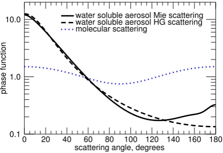
Fig. 1: Phase functions at 550 nm for molecules and dry water soluble aerosols derived from the Henyey-Greenstein (HG) approximation with g550 nmaer = 0.63 and the exact

Lorenz-Mie theory.

The transmitted light is scattered in all directions. The ra-tio of scattering to total light extincra-tionωλand the angular

distribution of the scattered lightPλ(Θ)are used to describe

the scattering process. To simplify the approach, the total intrinsic atmospheric scattering function can be decomposed into the single scattering approximation (SSA) and multiple scattering (MS). The first order atmospheric reflectance func-tionRI_λ,SSAcan be expressed using the analytical equation as given in van de Hulst (1948); Sobolev (1972); Hansen and Travis (1974); Kokhanovsky (2006):

RI_λ,SSA=ω

mlc

λ Pλmlc(Θ) 4(µ0+µ)

1−e−mτλI

, (9)

where the molecular single scattering albedoω_λmlc:= 1and the molecular (Rayleigh) scattering phase function for re-flected, unpolarised solar radiation is given by:

Pλmlc(Θ) = 3

4 1 + cos

2_Θ

, (10)

with the scattering angle

Θ = arccosh−µ0µ+ cos(φ−φ0) p

(1−µ0)(1−µ) i

(11)

and the geometrical air mass factor m= µ−₀1+µ−1

.

P_λmlc(Θ)is plotted in Fig. 1.

Standard RTMs spend most of their computational time calculating multiple scattering with iterative integration pro-cedures. In the case of layer I, we therefore suggest a generic correction factorfcorr_{to approximate Rayleigh}

mul-tiple scattering. We derive onefcorr per SZA as a function ofλandτfrom accurate MODTRAN/DISORT calculations, however without polarisation. The correction factor is de-fined as the ratio between the total reflectance and the SSA at sensor level:

f_µ0corr(λ,τ) = R

sensor,MODTRAN λ

Rsensor_λ ,SSA,MODTRAN. (12)

The total reflectance function of layer I is then given by Eqs. (9) and (12):

RIλ=R I,mlc

λ =

ωmlc_λ P_λmlc(Θ) 4(µ0+µ)

1−e−mτλI

fµcorr0 . (13) 2.2 Radiative transfer in layer II

The down- and upward total transmittances T_λII↓, T_λII↑ in layer II are calculated according to Eq. (4) by usinggaer

λ and

substitutingτI

λto the total spectral optical depth of layer II τ_λII=τ_λaer+τ_λmlchPBL.

The atmospheric reflectance function of layer II is sim-plified by the decomposition into molecular and aerosol parts. As a consequence, the aerosol-molecule scattering interactions are neglected. The related error is examined in Sect. 3.3. The molecular reflectance function RII_λ,mlc

is derived directly from Eq. (13), where τI

λ is changed to τmlc

λ hPBL. Thus, the total reflectance function of layer II

is given by:

RII_λ=R_λII,mlc+

first order scattering (SSA)

z }| {

ωaer λ P

aer λ (Θr)

4(µ0+µ)

1−e−mτλaer

+

second order z }| {

Raer_λ ,MS

| {z }

Raer

λ

.(14)

The aerosol scattering phase function Paer

λ (Θ) is defined

by the approximate Henyey-Greenstein (HG) phase func-tion (Henyey and Greenstein, 1941), which depends on the aerosol asymmetry factorgaer

λ and the scattering angleΘ:

Pλaer(Θ) =

1−(g_λaer)2

h

1 + (gaer λ )

2 −2gaer

λ cosΘ

i2/3. (15)

This HG phase function is plotted in Fig. 1 withgaer 550 nm=

0.63for a dry water soluble aerosol according to d’Almeida et al. (1991). The exact phase function derived from the Lorenz-Mie theory is superimposed to illustrate the imper-fection of the HG approximation in the forward scattering domain for Θ>150◦_{. This influence on the accuracy of}

SMART is discussed in the second half of Sect. 3.2.

The second order (or secondary) scattering is calculated according to the Successive Orders of Scattering (SOS) method described by Hansen and Travis (1974):

Raer,MS(µ,µ0,φ−φ0) =

τaerωaer

4π (16)

· 2π Z 0 1 Z 0 1 µP aer

t (µ,µ0,φ−φ0)R

SSA₍_µ0_,µ

0,φ0−φ0)

+ 1 µ0

RSSA(µ,µ0,φ−φ0)P_taer(µ0,µ0,φ0−φ0)

−e −τaer

µ₀

µ0

TSSA(µ,µ0,φ−φ0)P_raer(µ0,µ0,φ0−φ0)

−e −τaer

µ

µ P

aer

r (µ,µ0,φ−φ0)T

SSA₍_µ0_,µ

0,φ0−φ0) #

dµ0dφ0.

Fig. 1. Phase functions at 550 nm for molecules and dry water solu-ble aerosols derived from the Henyey-Greenstein (HG) approxima-tion withg_550nmaer =0.63 and the exact Lorenz-Mie theory.

The transmitted light is scattered in all directions. The ra-tio of scattering to total light extincra-tionωλ and the angular distribution of the scattered lightPλ(2)are used to describe the scattering process. To simplify the approach, the total intrinsic atmospheric scattering function can be decomposed into the single scattering approximation (SSA) and multiple scattering (MS). The first order atmospheric reflectance func-tionR_λI,SSAcan be expressed using the analytical equation as given in van de Hulst (1948); Sobolev (1972); Hansen and Travis (1974); Kokhanovsky (2006):

R_λI,SSA=ω mlc λ P

mlc λ (2) 4(µ0+µ)

1−e−mτλI

, (9)

where the molecular single scattering albedoω_λmlc:=1 and the molecular (Rayleigh) scattering phase function for re-flected, unpolarised solar radiation is given by:

P_λmlc(2)=3 4

1+cos22, (10)

with the scattering angle

2=arccosh−µ0µ+cos(φ−φ0)

p

(1−µ0)(1−µ)

i

(11)

and the geometrical air mass factor m=µ−₀1+µ−1. P_λmlc(2)is plotted in Fig. 1.

Standard RTMs spend most of their computational time calculating multiple scattering with iterative integration pro-cedures. In the case of layer I, we therefore suggest a generic correction factorfcorrto approximate Rayleigh mul-tiple scattering. We derive onefcorrper SZA as a function ofλandτ from accurate MODTRAN/DISORT calculations, however without polarisation. The correction factor is

de-fined as the ratio between the total reflectance and the SSA at sensor level:

f_µcorr

0 (λ,τ )=

R_λsensor,MODTRAN R_λsensor,SSA,MODTRAN

. (12)

The total reflectance function of layer I is then given by Eqs. (9) and (12):

R_λI=R_λI,mlc=ω mlc λ P

mlc λ (2) 4(µ0+µ)

1−e−mτλI

f_µcorr

0 . (13)

2.2 Radiative transfer in layer II

The down- and upward total transmittances T_λII↓, T_λII↑ in layer II are calculated according to Eq. (4) by usinggaer_λ and substitutingτ_λI to the total spectral optical depth of layer II τ_λII=τ_λaer+τ_λmlchPBL.

The atmospheric reflectance function of layer II is sim-plified by the decomposition into molecular and aerosol parts. As a consequence, the aerosol-molecule scattering interactions are neglected. The related error is examined in Sect. 3.3. The molecular reflectance function RII_λ,mlc is derived directly from Eq. (13), where τ_λI is changed to τ_λmlchPBL. Thus, the total reflectance function of layer II is given by:

R_λII=R_λII,mlc+

first order scattering(SSA)

z }| {

ωaer_λ P_λaer(2r) 4(µ0+µ)

1−e−mτλaer

+

second order

z }| {

Raer_λ ,MS

| {z }

R_λaer

.(14)

The aerosol scattering phase function P_λaer(2) is defined by the approximate Henyey-Greenstein (HG) phase func-tion (Henyey and Greenstein, 1941), which depends on the aerosol asymmetry factorg_λaerand the scattering angle2:

P_λaer(2)= 1− g aer λ

2 h

1+ gaer_λ 2₋

2gaer_λ cos2i2/3

. (15)

This HG phase function is plotted in Fig. 1 withgaer_550nm= 0.63 for a dry water soluble aerosol according to d’Almeida et al. (1991). The exact phase function derived from the Lorenz-Mie theory is superimposed to illustrate the imper-fection of the HG approximation in the forward scattering domain for 2 >150◦_{. This influence on the accuracy of}

SMART is discussed in the second half of Sect. 3.2.

The second order (or secondary) scattering is calculated according to the Successive Orders of Scattering (SOS)

(4)

method described by Hansen and Travis (1974): Raer,MS(µ,µ0,φ−φ0)=

τaerωaer

4π (16)

· 2π

Z

0 1

Z

0

₁

µP aer t µ,µ

0

,φ−φ0RSSA µ0,µ0,φ0−φ0

+ 1 µ0

RSSA µ,µ0,φ−φ0P_taer µ0,µ0,φ0−φ0

−e

−τ_µaer

0 µ0

TSSA µ,µ0,φ−φ0

P_raer µ0,µ0,φ0−φ0

−e

−τaer

µ

µ P

aer r µ,µ

0_,φ₋_φ0

TSSA µ0,µ0,φ0−φ0



dµ 0_dφ0_.

λand other non-angular arguments are omitted for the sake of readability. P_raer andP_taer denote the aerosol HG phase function (Eq. 15) using the scattering angle2r in case of reflectance (Eq. 11) and the scattering angle

2t=arccos

h

µ0µ+cos(φ−φ0)

p

(1−µ0)(1−µ)

i

(17) in case of transmittance. The single scattering transmit-tanceTSSAis given in van de Hulst (1948); Sobolev (1972); Hansen and Travis (1974); Kokhanovsky (2006):

T_λSSA=ω aer

λ Pλaer(2t) 4(µ0−µ)

e−

τaer

λ

µ₀ ₋_e−

τ_λaer

µ

!

. (18)

In case ofµ0=µ, we modify Eq. (18) to avoid indeterminacy with l’Hˆopital’s (Bernoulli’s) rule:

T_λSSA=ω aer

λ Pλaer(2t) 4µ2 τ

aer λ e

−τ

aer λ

µ

. (19)

We use a numerical approximation to calculate the inte-grals of Eq. (16). This is by far the most computation-ally intensive step in SMART. Therefore, we currently ne-glect scattering orders higher than two. A third order term could be added to Eq. (16) as given by Hansen and Travis (1974). However, for our accuracy requirements and under favourable remote sensing conditions, second order scatter-ing is sufficient. More details are given in the first half of Sect. 3.2.

If fast computation is more important than accuracy, R_λaer,MScan be substituted by·f_µcorr

0 λ,τ aer 550nm

in analogy to Eq. (12). The expense is roughly 20% in decreased accuracy. 2.3 Radiative transfer at the surface

The modelling of optical processes at the surface can be elaborate due to adjacency and directional effects. Here we assume the simple case with isotropically reflected light on a homogeneous surface according to Lambert’s law ( ˚Angstr¨om, 1925; Chandrasekhar, 1960; Sobolev, 1972): R_λSFC= aλ

1−sλaλ

, (20)

where aλ is the surface albedo and sλ is the spherical albedo to account for multiple interaction between surface and atmosphere. We use the parameterization suggested by Kokhanovsky et al. (2005) forsλ, where:

sλ=τIIλ ae

−τ

II λ

α +be−

τ_λII

β +c

!

. (21)

The constants a, α, b, β andc are parameterized accord-ing to Eq. (8). The correspondaccord-ing expansion coefficients are given in Kokhanovsky et al. (2005). The resultingRSFC_λ is also known as the hemispherical conical reflectance factor (HCRF) according to Schaepman-Strub et al. (2006). 2.4 At-sensor reflectance function

Finally, we put the above equations together along the optical path to resolve the reflectance functionR_λS. Multiple retro-reflections between layers I and II are neglected. A sensor at TOA or within levels I or II is simulated as follows:

R_λS,TOA=RI_λ+T_λI↓hR_λII+R_λSFCT_λIIliT_λI↑, (22)

RS_λ,I=R_λIshI+T_λI↓

h

RII_λ+R_λSFCT_λIIl

i

1−shI+shIT_λI↑

,(23)

R_λS,II=T_λI↓hR_λIIshII+T_λII↓R_λSFC1−shII+shIIT_λII↑i.(24) whereT_λIIl:=T_λII↓T_λII↑,

shI=p

PBL₋_pSensor

pPBL₋_pTOA and sh

II₌pSFC−pSensor

pSFC₋_pPBL . (25) These scaling factors are used to account for the relative height of the sensor within the corresponding layer. shI ranges from 1 at TOA to 0 at the PBL, whileshIIvaries from 1 at the PBL to 0 at the Earth’s surface (SFC).

3 Accuracy assessment

For typical airborne remote sensing conditions in the mid-latitudes we choose the representative uncertainty of imaging spectroscopy data of approximately 5% (Itten et al., 2008) as the accuracy requirement for SMART. Less typical con-ditions are analysed as well; in these cases we will accept larger errors. The definition of the conditions is given in Table 1. The AOD range was chosen according to the find-ings of Ruckstuhl et al. (2008), the wavelength range selected with regard to the optimal sensor performance (Seidel et al., 2008), while also avoiding strong water vapour absorption. We assume a black surface at the sea level (aλ=0) to focus on the atmospheric part of SMART. Furthermore, we solely use the nadir viewing direction (µ=1), which is approximated by small field-of-view sensors (FOV<30◦).

This section evaluates if the prior accuracy require-ments can be met by SMART. We compare SMART with

(5)

F. C. Seidel et al.: Fast and simple model for atmospheric radiative transfer 1133

Table 1. Definition of the conditions and the related accuracy re-quirements for SMART. The limited conditions refer to typical air-borne remote sensing needs in the mid-latitudes, which SMART was developed for. The analysed conditions refer to the accuracy assessment.

remote sensing conditions limited analysed

τ_550nmaer 0–0.5 0–0.5 solar zenith angle, degrees 20–60 nadir–70 viewing zenith angle nadir nadir wavelength, nm 500–700 400–800

surface albedo 0 0

accuracy requirement, % 5 15

an assumed virtual truth computed by the well known RTM 6SV1.1. It accounts for polarisation and uses the SOS method as well as aerosol phase matrices based on Lorenz-Mie scattering theory (Vermote et al., 1997). It was validated and found to be consistent to within 1% when compared to other RTMs by Kotchenova et al. (2006). We use the de-fault accuracy mode of 6S with 48 Gaussian scattering angles and 26 atmospheric layers. The use of more calculation an-gles and layers would be possible, but the accuracy increase would be 0.4% at best (Kotchenova et al., 2006) and there-fore is negligible for our study. The two layers of SMART were chosen to interface at 2 km above the surface. The lower layer includes dry water soluble aerosols and molecules dis-tributed along the exponential vertical air pressure gradient. The corresponding aerosol optical parametersg_λaer,ω_λaerand αλ are taken from d’Almeida et al. (1991) for SMART and 6S. All results in this study are calculated with identical in-put parameters in SMART and in 6S, which are provided in Table 2.

In the following, the accuracy of SMART is investigated for specific approximation uncertainties, as well as for the overall accuracy. As an indicator of the accuracy, we calcu-late the relative difference or percent error of the reflectance function to the benchmark 6S:

δR·100=R S

SMART−R S 6S R_6SS

·100. (26)

3.1 Rayleigh scattering approximation and polarisation

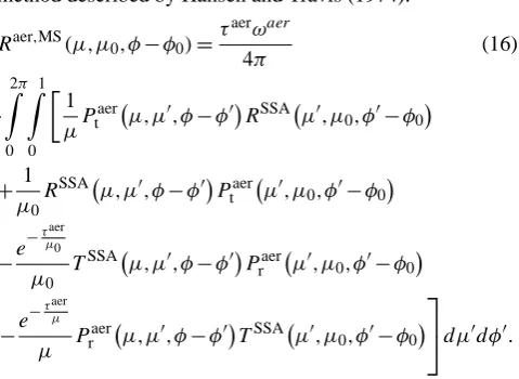
The total Rayleigh scattering is Rmlc_λ =RmlcI_λ +R_λmlcII as given by Eqs. (13) and (14). The associated approxima-tions include the Rayleigh scattering phase function (Eq. 10), the multiple scattering correction factor from MODTRAN (Eq. 12) and the neglected polarisation due to the scalar equa-tions. The percent error is a distinct function of the wave-length and SZA, induced mainly by polarisation. Figure 2a shows that it grows towards shorter wavelengths and larger

Table 2: Summary of the input parameters used in SMART and 6S for the accuracy assessment, with the aerosol and molecular optical depthτ_{550 nm}aer andτ_{550 nm}mlc , the solar and viewing zenith angle SZA and VZA, the aerosol asymmetry factor and single scattering albedogaer

550 nmandωaer550 nm, the ˚Angstr¨om parameterα550 nm, the surface albedoaλ, as well as the air pressure at

the surface and the planetary boundary layerpSFC_and_pPBL_{and the corresponding scaling factor}_hPBL_.

parameter τ550 nmaer τ

mlc

550nm SZA VZA g

aer 550 nm ω

aer

550 nm α550 nm aλ pSFC pPBL hPBL

value 0–0.5 0.097 nadir–70◦ nadir 0.638 0.963 1.23 0 1013 mb 800 mb 0.211

the nadir viewing direction (µ=1), which is approximated by small field-of-view sensors (FOV<30◦).

This section evaluates if the prior accuracy require-ments can be met by SMART. We compare SMART with an assumed virtual truth computed by the well known RTM 6SV1.1. It accounts for polarisation and uses the SOS method as well as aerosol phase matrices based on Lorenz-Mie scattering theory (Vermote et al., 1997). It was validated and found to be consistent to within 1% when compared to other RTMs by Kotchenova et al. (2006). We use the de-fault accuracy mode of 6S with 48 Gaussian scattering angles and 26 atmospheric layers. The use of more calculation an-gles and layers would be possible, but the accuracy increase would be 0.4% at best (Kotchenova et al., 2006) and there-fore is negligible for our study. The two layers of SMART were chosen to interface at 2 km above the surface. The lower layer includes dry water soluble aerosols and molecules dis-tributed along the exponential vertical air pressure gradient. The corresponding aerosol optical parametersg_λaer,ω_λaerand

αλ are taken from d’Almeida et al. (1991) for SMART and

6S. All results in this study are calculated with identical in-put parameters in SMART and in 6S, which are provided in Table 2.

In the following, the accuracy of SMART is investigated for specific approximation uncertainties, as well as for the overall accuracy. As an indicator of the accuracy, we calcu-late the relative difference or percent error of the reflectance function to the benchmark 6S:

δR·100 =R

S

SMART−RS6S

RS 6S

·100. (26)

3.1 Rayleigh scattering approximation and polarisation

The total Rayleigh scattering is R_λmlc=RmlcI_λ +RmlcII_λ as given by Eqs. (13) and (14). The associated approxima-tions include the Rayleigh scattering phase function (Eq. 10), the multiple scattering correction factor from MODTRAN (Eq. 12) and the neglected polarisation due to the scalar equa-tions. The percent error is a distinct function of the wave-length and SZA, induced mainly by polarisation. Figure 2a shows that it grows towards shorter wavelengths and larger SZA. It is known that the scalar approximation can introduce

relative error, %

10

5

0

−5

−10

wavelength, nm

800 750 700 650 600 550 500 450 400

SZA=60 SZA=45 SZA=30 SZA=15

(a) δRmlc

λ (λ)·100

relative error, %

10

5

0

−5

−10

solar zenith angle, degrees20 30 40 50 60 70 10

0

AOD=0.0

(b) δRmlc

550 nm(SZA)·100atλ= 550 nm

Fig. 2: Percent error due to Rayleigh scattering and polarisa-tion with respect to wavelength and solar zenith angle (SZA) at top-of-atmosphere.

uncertainties of up to 10% in the blue spectral region (van de Hulst, 1980; Mishchenko et al., 1994). The SZA depen-dency of this uncertainty is shown in Fig. 2b. At 550 nm, the Rayleigh scattering uncertainty in the typical SZA range from 20–50◦is below 3%.

Fig. 2. Percent error due to Rayleigh scattering and polarisation with respect to wavelength and solar zenith angle (SZA) at top-of-atmosphere.

SZA. It is known that the scalar approximation can introduce uncertainties of up to 10% in the blue spectral region (van de Hulst, 1980; Mishchenko et al., 1994). The SZA depen-dency of this uncertainty is shown in Fig. 2b. At 550 nm, the Rayleigh scattering uncertainty in the typical SZA range from 20–50◦is below 3%.

3.2 Aerosol scattering approximation

The main approximations for the aerosol scattering are the double scattering (Eq. 16) and the HG phase function (Eq. 15). Initially, we use the exactly same phase function as in 6S in order to study the error induced only by the ne-glected higher orders of scattering. This phase function for dry water soluble aerosols was derived from the Lorenz-Mie scattering theory. Subsequently, we compare the combined

(6)

Table 2. Summary of the input parameters used in SMART and 6S for the accuracy assessment, with the aerosol and molecular optical depth

τ_550nmaer andτ_{550 nm}mlc , the solar and viewing zenith angle SZA and VZA, the aerosol asymmetry factor and single scattering albedogaer_{550 nm}

andωaer_{550 nm}, the ˚Angstr¨om parameterα550 nm, the surface albedoaλ, as well as the air pressure at the surface and the planetary boundary layerpSFCandpPBLand the corresponding scaling factorhPBL.

parameter τ_550nmaer τ_550nmmlc SZA VZA g_550nmaer ωaer_550nm α550nm aλ pSFC pPBL hPBL value 0–0.5 0.097 nadir–70◦ nadir 0.638 0.963 1.23 0 1013 mb 800 mb 0.211

effect of the double scattering and the HG phase function ap-proximation with 6S.

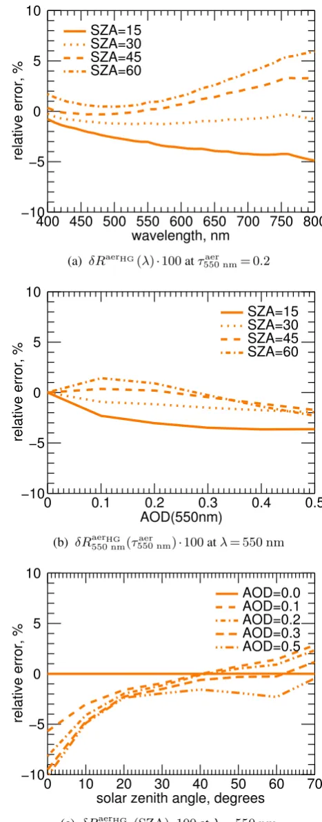
The percent error introduced by the double scattering ap-proximation is plotted in Fig. 3. It is almost constant over the spectra due to the higher reflectance at shorter wavelengths (see Fig. 3a). It is obvious that the reflectance functionRS_λis increasingly underestimated by SMART for larger AOD due to the neglected third and higher orders of aerosol scattering (see Fig. 3b). Figure 3c shows that larger SZA leads to an underestimation of the atmospheric reflectance for the same reason.

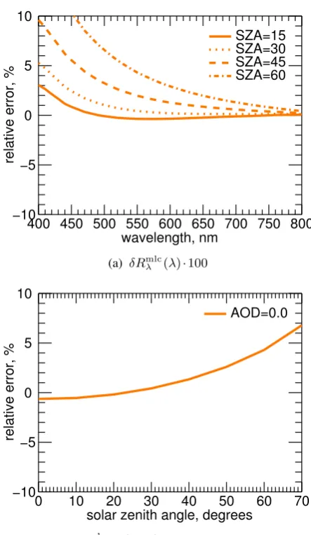
In order to study the accuracy of the total aerosol scatter-ingRaer_λ as part of Eq. (14), we include the approximative HG phase function in SMART. 6S still uses the same Mie phase function as before. The input parameter for the HG phase functiongaer_λ corresponds to the same dry water sol-uble aerosol, which is used in 6S. The exact Mie and the approximative HG phase function are shown in Fig. 1 for the same aerosol. The latter provides a reasonable approxima-tion for scattering angles around 130◦, which corresponds to a 50◦SZA for nadir observations. The resulting combination of the aerosol double scattering error with the HG approxi-mation error is examined in Fig. 4. It suggests that the use of the HG approximation does not introduce large percent er-rors within the range of typical SZA, as defined in Table 1. Given a range of 20–45◦SZA, SMART is quite accurate at all investigated wavelengths and AOD values.

By comparing Figs. 3a with 4a and Figs. 3b with 4b, it can be seen that the HG approximation reverses some of the er-rors due to the aerosol double scattering approximation. The HG phase function for dry water soluble aerosols tends to overestimate of the aerosol scattering, which finally leads to a less distinct underestimation due to the neglected third and higher orders of aerosol scattering.

3.3 Coupling of Rayleigh and aerosol scattering The current version of SMART does not yet account for the scattering interaction between molecules and aerosols. We analyse this effect by comparing 6S computations with the coupling switched on and off. The relative error related to this specific approximation is shown in Fig. 5. It remains within about 3%, reaching a maximum at large SZA (see Fig. 5c) and short wavelengths (see Fig. 5a). With errors

of less than 2%, small SZAs are almost not influenced by the coupling and there is no distinct dependency on AOD notice-able (see Fig. 5b).

3.4 Overall accuracy

Previous Sects. 3.1–3.3 demonstrated that the approxima-tions in SMART are adequate. Most of them are within the desired accuracy range of±5% for the limited remote sens-ing conditions as defined in Table 1. Errors of up to±15% are found for large SZA, however, they are mainly related to SMART’s simple two-layer atmospheric structure.

In the following, we examine the overall accuracy of SMART by comparing it according to Eq. (26) with inde-pendent computations of 6S. The computations of SMART are performed by Eq. (22) for a TOA sensor altitude at 80 km and by Eq. (23) for an airborne sensor altitude at 5500 m a.s.l. The percent error due to the excluded coupling between molecules and aerosols is inherent in the results of this sub-section.

Figure 6 shows the result of two independent calculations using SMART (solid line) and 6S (dashed line) with respect toλandτ_550nmaer . The qualitative agreement between the two models is evident. A quantitative perspective by statistical means of the overall accuracy is provided in Table 3, where R2=1−

P

R_SMARTS −RS_6S2

P_RS

6S− ¯RS6S

2 , (27)

is the squared correlation coefficient between the two models,

RMSE=

r

1 N

X

R_SMARTS −RS_6S2

, (28)

is the root mean square error and

NRMSE= RMSE·100

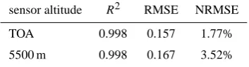
max RS_SMART−min RS_SMART, (29) is the normalised RMSE. The statistics are derived from all combinations of input parameters defined in Tables 1 and 2 within the limited conditions. The resulting correlation be-tween SMART and 6S is almost perfect. The RMSE is ap-proximately 0.16 reflectance values and the NRMSE is be-tween 1.8% and 3.5%. The differences are smaller at TOA in comparison to those at 5500 m.

(7)

6 F. C. Seidel et al.: Fast and simple model for atmospheric radiative transfer

3.2 Aerosol scattering approximation

The main approximations for the aerosol scattering are the double scattering (Eq. 16) and the HG phase function (Eq. 15). Initially, we use the exactly same phase function as in 6S in order to study the error induced only by the ne-glected higher orders of scattering. This phase function for dry water soluble aerosols was derived from the Lorenz-Mie scattering theory. Subsequently, we compare the combined effect of the double scattering and the HG phase function ap-proximation with 6S.

The percent error introduced by the double scattering ap-proximation is plotted in Fig. 3. It is almost constant over the spectra due to the higher reflectance at shorter wavelengths (see Fig. 3a). It is obvious that the reflectance functionRS

λis

increasingly underestimated by SMART for larger AOD due to the neglected third and higher orders of aerosol scattering (see Fig. 3b). Figure 3c shows that larger SZA leads to an underestimation of the atmospheric reflectance for the same reason.

In order to study the accuracy of the total aerosol scatter-ing Raer_λ as part of Eq. (14), we include the approximative HG phase function in SMART. 6S still uses the same Mie phase function as before. The input parameter for the HG phase function g_λaer corresponds to the same dry water sol-uble aerosol, which is used in 6S. The exact Mie and the approximative HG phase function are shown in Fig. 1 for the same aerosol. The latter provides a reasonable approxima-tion for scattering angles around 130◦, which corresponds to a 50◦SZA for nadir observations. The resulting combination of the aerosol double scattering error with the HG approxi-mation error is examined in Fig. 4. It suggests that the use of the HG approximation does not introduce large percent er-rors within the range of typical SZA, as defined in Table 1. Given a range of 20–45◦SZA, SMART is quite accurate at all investigated wavelengths and AOD values.

By comparing Fig. 3a with 4a and Fig. 3b with 4b, it can be seen that the HG approximation reverses some of the er-rors due to the aerosol double scattering approximation. The HG phase function for dry water soluble aerosols tends to overestimate of the aerosol scattering, which finally leads to a less distinct underestimation due to the neglected third and higher orders of aerosol scattering.

3.3 Coupling of Rayleigh and aerosol scattering

The current version of SMART does not yet account for the scattering interaction between molecules and aerosols. We analyse this effect by comparing 6S computations with the coupling switched on and off. The relative error related to this specific approximation is shown in Fig. 5. It remains within about 3%, reaching a maximum at large SZA (see Fig. 5c) and short wavelengths (see Fig. 5a). With errors of less than 2%, small SZAs are almost not influenced by the

relative error, %

10

5

0

−5

−10

wavelength, nm550 600 650 700 750 800 500 450 400 SZA=60 SZA=45 SZA=30 SZA=15

(a) δRaerMie₍_λ₎_·₁₀₀_at_τaer

550 nm= 0.2

relative error, %

10 5 0 −5 −10 AOD(550nm) 0.5 0.4 0.3 0.2 0.1 0 SZA=60 SZA=45 SZA=30 SZA=15

(b) δRaerMie 550 nm(τ

aer

550 nm)·100atλ= 550 nm

relative error, %

10

5

0

−5

−10

solar zenith angle, degrees20 30 40 50 60 70 10 0 AOD=0.5 AOD=0.3 AOD=0.2 AOD=0.1 AOD=0.0

(c) δRaerMie

550 nm(SZA)·100atλ= 550 nm

Fig. 3: Percent error of the SMART reflectance function due to aerosol scattering with respect to wavelength, aerosol op-tical depth (AOD) and solar zenith angle (SZA) at top-of-atmosphere. SMART and 6S use the same phase function from Lorenz-Mie theory.

Fig. 3. Percent error of the SMART reflectance function due to aerosol scattering with respect to wavelength, aerosol optical depth (AOD) and solar zenith angle (SZA) at top-of-atmosphere. SMART and 6S use the same phase function from Lorenz-Mie theory.

relative error, %

10 5 0 −5 −10 wavelength, nm 800 750 700 650 600 550 500 450 400 SZA=60 SZA=45 SZA=30 SZA=15

(a) δRaerHG₍_λ₎_·₁₀₀_at_τaer

550 nm= 0.2

relative error, %

10

5

0

−5

−10

AOD(550nm)0.2 0.3 0.4 0.5 0.1 0 SZA=60 SZA=45 SZA=30 SZA=15

(b) δRaerHG 550 nm(τ

aer

550 nm)·100atλ= 550 nm

relative error, %

10

5

0

−5

−10

solar zenith angle, degrees

70 60 50 40 30 20 10 0 AOD=0.5 AOD=0.3 AOD=0.2 AOD=0.1 AOD=0.0

(c) δRaerHG

550 nm(SZA)·100atλ= 550 nm

Fig. 4: Percent error of the SMART reflectance function due to aerosol scattering with respect to wavelength, aerosol op-tical depth (AOD) and solar zenith angle (SZA) at top-of-atmosphere. SMART uses the HG phase function, 6S the phase function from Lorenz-Mie theory.

relative error, %

10 5 0 −5 −10 wavelength, nm 800 750 700 650 600 550 500 450 400 SZA=60 SZA=45 SZA=30 SZA=15

(a) δRmlc+aer(λ)·100atτ550 nmaer = 0.3

relative error, %

(b) δRmlc+aer550 nm (τ aer

550 nm)·100atλ= 550 nm

relative error, %

10

5

0

−5

−10

solar zenith angle, degrees

70 60 50 40 30 20 10 0 AOD=0.5 AOD=0.3 AOD=0.2 AOD=0.1 AOD=0.0

(c) δRmlc+aer550 nm (SZA)·100atλ= 550 nm

Fig. 5: . Percent error due to the non-coupling approximation with respect to wavelength, aerosol optical depth (AOD) and solar zenith angle (SZA) at top-of-atmosphere.

Fig. 4. Percent error of the SMART reflectance function due to aerosol scattering with respect to wavelength, aerosol optical depth (AOD) and solar zenith angle (SZA) at top-of-atmosphere. SMART uses the HG phase function, 6S the phase function from Lorenz-Mie theory.

(8)

1136 F. C. Seidel et al.: Fast and simple model for atmospheric radiative transfer

relative error, %

10

5

0

−5

−10

(a) δRaerHG₍_λ₎_·₁₀₀_at_τaer

550 nm= 0.2

relative error, %

10

5

0

−5

−10

AOD(550nm)0.2 0.3 0.4 0.5 0.1 0 SZA=60 SZA=45 SZA=30 SZA=15

(b) δRaerHG 550 nm(τ

aer

550 nm)·100atλ= 550 nm

relative error, %

10

5

0

−5

−10

(c) δRaerHG

550 nm(SZA)·100atλ= 550 nm

Fig. 4: Percent error of the SMART reflectance function due to aerosol scattering with respect to wavelength, aerosol op-tical depth (AOD) and solar zenith angle (SZA) at top-of-atmosphere. SMART uses the HG phase function, 6S the phase function from Lorenz-Mie theory.

relative error, %

10

5

0

−5

−10

(a) δRmlc+aer(λ)·100atτ550 nmaer = 0.3

relative error, %

(b) δRmlc+aer550 nm (τ aer

550 nm)·100atλ= 550 nm

relative error, %

10

5

0

−5

−10

(c) δR550 nmmlc+aer(SZA)·100atλ= 550 nm

Fig. 5: . Percent error due to the non-coupling approximation with respect to wavelength, aerosol optical depth (AOD) and solar zenith angle (SZA) at top-of-atmosphere.

Fig. 5. Percent error due to the non-coupling approximation with respect to wavelength, aerosol optical depth (AOD) and solar zenith angle (SZA) at top-of-atmosphere.

coupling and there is no distinct dependency on AOD notice-able (see Fig. 5b).

3.4 Overall accuracy

Previous Sects. 3.1–3.3 demonstrated that the approxima-tions in SMART are adequate. Most of them are within the desired accuracy range of±5%for the limited remote sens-ing conditions as defined in Table 1. Errors of up to±15%

are found for large SZA, however, they are mainly related to SMART’s simple two-layer atmospheric structure.

In the following, we examine the overall accuracy of SMART by comparing it according to Eq. (26) with inde-pendent computations of 6S. The computations of SMART are performed by Eq. (22) for a TOA sensor altitude at 80 km and by Eq. (23) for an airborne sensor altitude at 5500 m a.s.l. The percent error due to the excluded coupling between molecules and aerosols is inherent in the results of this sub-section.

Figure 6 shows the result of two independent calculations using SMART (solid line) and 6S (dashed line) with respect toλandτaer

550 nm. The qualitative agreement between the two

models is evident. A quantitative perspective by statistical means of the overall accuracy is provided in Table 3, where

R2= 1− P

RS

SMART−RS6S 2

P

RS

6S−R¯S6S

2 , (27)

is the squared correlation coefficient between the two mod-els, RMSE = r 1 N X RS

SMART−RS6S 2

, (28)

is the root mean square error and

NRMSE = RMSE·100

max RS SMART

−min RS SMART

, (29)

is the normalised RMSE. The statistics are derived from all combinations of input parameters defined in Tables 1 and 2 within the limited conditions. The resulting correlation be-tween SMART and 6S is almost perfect. The RMSE is ap-proximately 0.16 reflectance values and the NRMSE is be-tween 1.8% and 3.5%. The differences are smaller at TOA in comparison to those at 5500 m.

In the following, we analyse the overall accuracy of Eq. (22) by Eq. (26) in more details with respect to wave-length, SZA and AOD. SMART computes very similar re-sults compared to 6S at TOA with an SZA between 30◦and 40◦. This conclusion can be drawn from the combination of Figs. 2b, 4c and 5c, as well as from the total percent error in Fig. 7a. The overall percent error does not exceed±5% at any investigated wavelength or AOD. At the large SZA of 60◦, SMART overestimates RS_λ,TOA by more than 10% at short wavelengths. Nevertheless, the overall accuracy is

Table 3: Quantitative comparison between SMART and 6S by statistical means for the limited conditions as defined in Table 1. SMART uses the HG phase function; 6S used the phase function from Mie calculations. R2 denotes the squared correlation coefficient, RMSE the root mean square error and NRMSE the normalised RMSE.

sensor altitude R2 RMSE NRMSE

TOA 0.998 0.157 1.77%

5500 m 0.998 0.167 3.52%

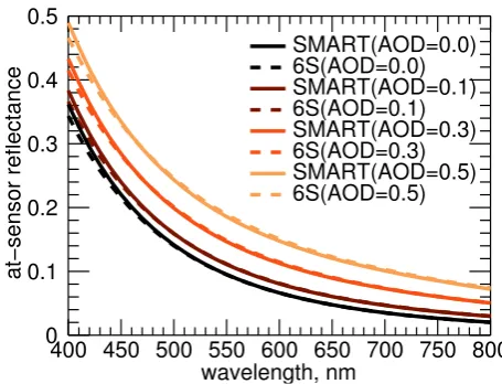
at−sensor reflectance 0.5 0.4 0.3 0.2 0.1 0 wavelength, nm 800 750 700 650 600 550 500 450 400 6S(AOD=0.5) SMART(AOD=0.5) 6S(AOD=0.3) SMART(AOD=0.3) 6S(AOD=0.1) SMART(AOD=0.1) 6S(AOD=0.0) SMART(AOD=0.0)

Fig. 6: Results of the at-sensor reflectance functionRS_λ,TOA

(Eq. 22) computed by SMART (solid line) and 6S (dashed line) at TOA, SZA=30◦and varyingτ550 nmaer . SMART uses

the HG phase function, while 6S uses the phase function from Mie theory. Remaining input parameters are given in Table 2.

still well within the acceptable range of 10% at any wave-length larger than 450 nm (see Fig. 7b). At 550 nm, only the combination of very small SZA with a strong AOD or a high SZA with low AOD leads to a percent error just outside of the desired 5% margin (see Fig. 7c). In the blue part of the spectrum, high or low SZA lead to significant percent errors in a pure Rayleigh scattering atmosphere (see Fig. 7e). The same is true in an atmosphere containing aerosols, where the aerosols introduce additional percent errors in the red part of the spectrum for small SZAs (see Figs. 7d and 7f).

Since SMART is also intended for the use with airborne remote sensing data, we additionally analyse the overall ac-curacy of Eq. (23) by Eq. (26). We place the sensor at 5500 m above the assumed black surface at sea level. The airborne scenario is more sensitive to the approximative two-layer setup in SMART. The 26 atmospheric layers in 6S can bet-ter account for the vertically inhomogeneous atmosphere. In

Fig. 6. Results of the at-sensor reflectance function R_λS,TOA

(Eq. 22) computed by SMART (solid line) and 6S (dashed line) at TOA, SZA=30◦and varyingτ_550nmaer . SMART uses the HG phase function, while 6S uses the phase function from Mie theory. Re-maining input parameters are given in Table 2.

In the following, we analyse the overall accuracy of Eq. (22) by Eq. (26) in more details with respect to wave-length, SZA and AOD. SMART computes very similar re-sults compared to 6S at TOA with an SZA between 30◦_and

40◦_{. This conclusion can be drawn from the combination of}

Figs. 2b, 4c and 5c, as well as from the total percent error in Fig. 7a. The overall percent error does not exceed±5% at any investigated wavelength or AOD. At the large SZA of 60◦, SMART overestimatesR_λS,TOAby more than 10% at short wavelengths. Nevertheless, the overall accuracy is still well within the acceptable range of 10% at any wavelength larger than 450 nm (see Fig. 7b). At 550 nm, only the com-bination of very small SZA with a strong AOD or a high SZA with low AOD leads to a percent error just outside of the desired 5% margin (see Fig. 7c). In the blue part of the spectrum, high or low SZA lead to significant percent errors in a pure Rayleigh scattering atmosphere (see Fig. 7e). The same is true in an atmosphere containing aerosols, where the aerosols introduce additional percent errors in the red part of the spectrum for small SZAs (see Fig. 7d and f).

Since SMART is also intended for the use with airborne remote sensing data, we additionally analyse the overall ac-curacy of Eq. (23) by Eq. (26). We place the sensor at 5500 m above the assumed black surface at sea level. The airborne scenario is more sensitive to the approximative two-layer setup in SMART. The 26 atmospheric layers in 6S can bet-ter account for the vertically inhomogeneous atmosphere. In fact, the percent error is slightly larger in the airborne case in comparison with the TOA case. The error distribution in the contour plots of Fig. 8a–f show that SMART underes-timates the reflectance factors at 5500 m. Nevertheless, the hypothetical pure Rayleigh atmosphere still performs well,

(9)

(a) δRS,TOA₍_λ,τaer

550 nm)·100at 30 ◦

SZA (b) δRS,TOA₍_λ,τaer

550 nm)·100at 60 ◦

SZA

(c) δRS_{550 nm},TOA(SZA,τaer

550 nm)·100atλ= 550nm (d) δR S,TOA

(λ,SZA)·100atτ550 nmaer = 0.0

(e) δRS,TOA(λ,SZA)·100atτ550 nmaer = 0.2 (f) δRS,TOA(λ,SZA)·100atτ550 nmaer = 0.5

Fig. 7: Overall accuracy with a sensor at top-of-atmosphere.

Fig. 7. Overall accuracy with a sensor at top-of-atmosphere.

(10)

Table 3. Quantitative comparison between SMART and 6S by statistical means for the limited conditions as defined in Table 1. SMART uses the HG phase function; 6S used the phase function from Mie calculations. R2 denotes the squared correlation coef-ficient, RMSE the root mean square error and NRMSE the nor-malised RMSE.

sensor altitude R2 RMSE NRMSE

TOA 0.998 0.157 1.77%

5500 m 0.998 0.167 3.52%

with a maximum percent error of 6% (see Fig. 8a, b and c). The aerosols worsen the underestimation in the lower half of the visible spectrum, especially at very small and very large SZAs. At 550 nm and a 30◦ SZA, the percent error is 6% or less for an AOD up to 0.5. With the same constellation but an extreme SZA, the percent errors reach about 10% (see Fig. 8c, e and f). The largest offset between SMART and 6S is found at 60◦SZA, 400 nm and an AOD of 0.5 with 18% relative difference. However, it should be noted that absolute differenceR_SMARTS −R_6SS is in fact smaller in the airborne case compared to the TOA case (not shown). Nonetheless, the relative error given by Eq. (26) is larger due to the smaller R_6SS in the denominator.

4 Performance assessment

SMART is designed to optimally balance the opposing needs for accuracy and computational speed; the speed decreases with increasing model complexity and accuracy. We use the 6S vector version 1.1 (Vermote et al., 1997) as a benchmark RTM (same as in Sect. 3) to assesses the performance of SMART. 6S is compiled with GNU Fortran and SMART is implemented in IDL. Both run on the same CPU infrastruc-ture.

SMART needs only approximately 0.05 s for the calcu-lation of one reflectance factor value. The more com-plex 6S needs about 1.4 s under identical conditions. Con-sequently, SMART computes more than 25 times faster. If R_λaer,MS (Eq. 16) is substituted by a simple correction factor f_µcorr

0 (λ,τ )for aerosol multiple scattering (similar to Eq. 12), SMART runs 220 times faster than by numerically solving Eq. (16) in the presented configuration.

5 Summary and conclusions

We introduced SMART, as well as its approximative radia-tive transfer equations and parameterizations. Results of the atmospheric at-sensor reflectance function computed by SMART were compared with benchmark results from 6S for

accuracy and performance. The overall percent error was ex-amined and discussed, as were the individual errors resulting from Rayleigh scattering, aerosol scattering and molecule-aerosol interactions. The molecule-aerosol scattering was compared to 6S with and without the effect of the HG phase function approximation.

We found that SMART fulfils its design principle: it is fast and simple, yet accurate enough for a range of applications. One example may include the assessment of atmospheric ef-fects when inspecting the quality of airborne or spaceborne data against ground truth measurements in near-real-time. The generation of atmospheric input parameters for vegeta-tion canopy RTM inversion schemes, could be another appli-cation. SMART computes more than 20 reflectance results per second on a current customary desktop computer. This is more than 25 times faster than the benchmark RTM. The overall percent error under typical mid-latitude remote sens-ing conditions was found to be about 5% for the spaceborne and 5% to 10% for the airborne case. Large AOD or SZA values lead to larger percent errors of up to 15%. In gen-eral, the included approximations are sensitive to the strong scattering in the blue spectral region, which leads to larger percent errors. Together with the effect of polarisation, the total percent error of SMART exceeds the desired accuracy goal of 5% only in the blue region. It is therefore suggested that SMART be used preferably in the spectral range between roughly 500 nm and 680 nm, avoiding the blue and strong ab-sorption bands. However, the neglected ozone abab-sorption in this spectral interval leads to a small overestimation of up to 0.007 reflectance units at large SZA and 600 nm. It is also recommended to use SMART for computations with a sensor above the PBL to avoid uncertainties in the vertical distribu-tion of the aerosols.

SMART can be improved by implementing other phase functions instead of the HG approximation, including those derived from Lorenz-Mie theory, geometrical optics (ray-tracing), and T-matrix approaches (Liou and Hansen, 1971; Mishchenko et al., 2002). Further refinements may include the coupling between molecules and aerosols, as well as the implementation of freely mixable aerosol components and hygroscopic growth (Hess et al., 1998). To account for polarisation, the scalar equations can be extended to the vector notation. Furthermore, a similar approach as used for the Rayleigh multiple scattering in this study (Eq. 12) may perhaps be used to perform a rough polarisation cor-rection. Other issues for further developments may include additional atmospheric layers, gaseous absorption (foremost ozone), adjacency effects and the treatment of a directional, non-Lambertian surface.

A recent inter-comparison study for classic RTMs such as 6S, RT3, MODTRAN and SHARM, found discrepancies of δR≤5% at TOA (Kotchenova et al., 2008). Even larger errors were found when polarisation was neglected or the HG phase function was used. SMART does not yet account for polari-sation and uses the HG approximation by default, however

(11)

(a) δRS,5500 m₍_λ,τaer

550 nm)·100at 30 ◦

SZA (b) δRS,5500 m₍_λ,τaer

550 nm)·100at 60 ◦

SZA

(c) δR_{550 nm}S,5500 m(SZA,τaer

550 nm)·100atλ= 550nm (d) δR

S,5500 m₍_λ,_SZA)_·₁₀₀

atτaer

550 nm= 0

(e) δRS,5500 m₍_λ,_SZA)_·₁₀₀

atτaer

550 nm= 0.2 (f) δRS,5500 m(λ,SZA)·100atτ550 nmaer = 0.5

Fig. 8: Overall accuracy with a sensor at 5500 m.

Fig. 8. Overall accuracy with a sensor at 5500 m.

(12)

with the option to include pre-calculated Mie phase func-tions. Therefore, the overall accuracy achieved by SMART under given conditions can be regarded as satisfactory, espe-cially when a computationally fast RTM is required.

Acknowledgements. The work of A. A. Kokhanovsky was per-formed in the framework of DFG Project Terra. Suggestions from D. Schlaepfer and A. Schubert were very much appreciated. We thank three anonymous referees for their valuable comments on the AMTD version of this publication.

Edited by: M. Wendisch

References ˚

Angstr¨om, A.: The albedo of various surfaces of ground, Ge-ogr. Ann., 7, 323–342, available at: http://www.jstor.org/stable/ 519495, last access: 1 May 2010, 1925.

˚

Angstr¨om, A.: On the atmospheric transmission of sun radiation and on dust in the air, Geogr. Ann., 11, 156–166, available at: http://www.jstor.org/stable/519399, last access: 1 May 2010, 1929.

Berk, A., Bernstein, L., and Robertson, D.: MODTRAN: a mod-erate resolution model for LOWTRAN7, Tech. Rep. GL-TR-89-0122, Air Force Geophysics Lab, Hanscom AFB, Massachusetts, USA, 1989.

Bodhaine, B. A., Wood, N. B., Dutton, E. G., and Slusser, J. R.: On Rayleigh optical depth calculations, J. At-mos. Ocean. Tech., 16, 1854–1861, doi:10.1175/1520-0426(1999)016<1854:ORODC>2.0.CO;2, 1999.

Carrer, D., Roujean, J.-L., Hautecoeur, O., and Elias, T.: Daily estimates of aerosol optical thickness over land sur-face based on a directional and temporal analysis of SEVIRI MSG visible observations, J. Geophys. Res., 115, D10208, doi:10.1029/2009JD012272, 2010.

Chandrasekhar, S.: Radiative Transfer, Dover, New York, USA, 1960.

d’Almeida, G., Koepke, P., and Shettle, E.: Atmospheric aerosols: global climatology and radiative characteristics, Deepak, Hamp-ton, Virginia, USA, 1991.

Evans, K. F. and Stephens, G. L.: A new polarized atmospheric radiative transfer model, J. Quant. Spectrosc. Ra., 46, 413–423, doi:10.1016/0022-4073(91)90043-P, 1991.

Gao, B.-C., Montes, M. J., Davis, C. O., and Goetz, A. F. H.: Atmo-spheric correction algorithms for hyperspectral remote sensing data of land and ocean, Remote Sens. Environ., 113, S17–S24, doi:10.1016/j.rse.2007.12.015, 2009.

Govaerts, Y.: RTMOM V0B.10 Evaluation report, report EUM/MET/DOC/06/0502, EUMETSAT, 2006.

Hammad, A. and Chapman, S.: VII. The primary and sec-ondary scattering of sunlight in a plane-stratified atmosphere of uniform composition, Philos. Mag., 28, 99–110, available at: http://articles.adsabs.harvard.edu//full/1948ApJ...108..338H/ 0000338.000.html, last access: 1 May 2010, 1939.

Hansen, J. E. and Travis, L. D.: Light scattering in planetary atmospheres, Space Sci. Rev., 16, 527–610, doi:10.1007/BF00168069, 1974.

Henyey, L. and Greenstein, J.: Diffuse radiation in the galaxy, As-trophys. J., 93, 70–83, available at: http://articles.adsabs.harvard. edu/full/1940AnAp....3..117H, last access: 1 May 2010, 1941. Hess, M., Koepke, P., and Schult, I.: Optical properties of aerosols

and clouds: the software package OPAC, B. Am. Meteorol. Soc., 79, 831–844, 1998.

Itten, K. I., Dell’Endice, F., Hueni, A., Kneubühler, M., Schläpfer, D., Odermatt, D., Seidel, F., Huber, S., Schopfer, J., Kellen-berger, T., Bühler, Y., D’Odorico, P., Nieke, J., Alberti, E., and Meuleman, K.: APEX – the hyperspectral ESA airborne prism experiment, Sensors, 8, 6235–6259, doi:10.3390/s8106235, available at: http://www.mdpi.com/1424-8220/8/10/6235, last access: 1 May 2010, 2008.

Katsev, I. L., Prikhach, A. S., Zege, E. P., Grudo, J. O., and Kokhanovsky, A. A.: Speeding up the AOT retrieval procedure using RTT analytical solutions: FAR code, Atmos. Meas. Tech. Discuss., 3, 1645–1705, doi:10.5194/amtd-3-1645-2010, 2010. Key, J. and Schweiger, A.: Tools for atmospheric radiative

trans-fer: Streamer and FluxNet, Comput. Geosci., 24, 443–451, doi:10.1016/S0098-3004(97)00130-1, 1998.

Kokhanovsky, A. A.: Cloud optics, Springer, Berlin, Germany, 276 pp., 2006.

Kokhanovsky, A. A.: Aerosol optics – Light Absorption and Scat-tering by Particles in the Atmosphere, Springer Praxis Books, Springer Berlin Heidelberg, 148 pp., 2008.

Kokhanovsky, A. A., Deuz´e, J. L., Diner, D. J., Dubovik, O., Ducos, F., Emde, C., Garay, M. J., Grainger, R. G., Heckel, A., Herman, M., Katsev, I. L., Keller, J., Levy, R., North, P. R. J., Prikhach, A. S., Rozanov, V. V., Sayer, A. M., Ota, Y., Tanr´e, D., Thomas, G. E., and Zege, E. P.: The inter-comparison of major satellite aerosol retrieval algorithms using simulated intensity and polar-ization characteristics of reflected light, Atmos. Meas. Tech., 3, 909–932, doi:10.5194/amt-3-909-2010, 2010.

Kokhanovsky, A. A. and de Leeuw, G.: Satellite aerosol re-mote sensing over land, Environmental Sciences, Springer Praxis Books, 388 pp., 2009.

Kokhanovsky, A. A., Mayer, B., and Rozanov, V. V.: A pa-rameterization of the diffuse transmittance and reflectance for aerosol remote sensing problems, Atmos. Res., 73, 37–43, doi:10.1016/j.atmosres.2004.07.004, 2005.

Kotchenova, S. Y., Vermote, E. F., Levy, R., and Lyapustin, A.: Radiative transfer codes for atmospheric correction and aerosol retrieval: intercomparison study, Appl. Optics, 47, 2215–2226, doi:10.1364/AO.47.002215, 2008.

Kotchenova, S. Y., Vermote, E. F., Matarrese, R., and Klemm, F. J.: Validation of a vector version of the 6S radiative transfer code for atmospheric correction of satellite data. Part I: Path radiance, Appl. Optics, 45, 6762–6774, doi:10.1364/AO.45.006762, 2006. Liou, K. and Hansen, J.: Intensity and polarization for single scat-tering by polydisperse sphere: A comparison of ray optics and Mie theory, J. Atmos. Sci., 28, 995–1004, doi:10.1175/1520-0469(1971)028<0995:IAPFSS>2.0.CO;2, 1971.

Lyapustin, A. I.: Radiative transfer code SHARM for atmo-spheric and terrestrial applications, Appl. Optics, 44, 7764–7772, doi:10.1364/AO.44.007764, 2005.

Mishchenko, M. I., Lacis, A. A., and Travis, L. D.: Errors in-duced by the neglect of polarization in radiance calculations for rayleigh-scattering atmospheres, J. Quant. Spectrosc. Ra., 51, 491–510, doi:10.1016/0022-4073(94)90149-X, 1994.

(13)

F. C. Seidel et al.: Fast and simple model for atmospheric radiative transfer 1141 Mishchenko, M. I., Travis, L. D., and Lacis, A. A.:

Scat-tering, absorption, and emission of light by small particles, Cambridge University Press, Cambridge, doi:10.1016/S0022-4073(98)00025-9, 2002.

Muldashev, T. Z., Lyapustin, A. I., and Sultangazin, U. M.: Spheri-cal harmonics method in the problem of radiative transfer in the atmosphere-surface system, J. Quant. Spectrosc. Ra., 61, 393– 404, doi:10.1016/S0022-4073(98)00025-9, 1999.

Nakajima, T. and Tanaka, M.: Matrix formulations for the transfer of solar radiation in a plane-parallel scattering atmo-sphere, J. Quant. Spectrosc. Ra., 35, 13–21, doi:10.1016/0022-4073(86)90088-9, 1986.

Ota, Y., Higurashi, A., Nakajima, T., and Yokota, T.: Matrix for-mulations of radiative transfer including the polarization effect in a coupled atmosphere–ocean system, J. Quant. Spectrosc. Ra., 111, 878–894, doi:10.1016/j.jqsrt.2009.11.021, 2010.

Ricchiazzi, P., Yang, S., Gautier, C., and Sowle, D.: SBDART: A research and teaching software tool for plane-parallel radiative transfer in the Earth’s atmosphere, B. Am. Meteorol. Soc., 79, 2101–2114, 1998.

Rozanov, A., Rozanov, V., Buchwitz, M., Kokhanovsky, A., and Burrows, J.: SCIATRAN 2.0 – A new radiative transfer model for geophysical applications in the 175–2400 nm spectral region, Adv. Space Res., 36, 1015–1019, doi:10.1016/j.asr.2005.03.012, 2005.

Ruckstuhl, C., Philipona, R., Behrens, K., Collaud Coen, M., D¨urr, B., Heimo, A., M¨atzler, C., Nyeki, S., Ohmura, A., Vuilleumier, L., Weller, M., Wehrli, C., and Zelenka, A.: Aerosol and cloud effects on solar brightening and the recent rapid warming, Geo-phys. Res. Lett., 35, L12708, doi:10.1029/2008GL034228, 2008. Ruggaber, A., Dlugi, R., and Nakajima, T.: Modelling radiation quantities and photolysis frequencies in the troposphere, J. At-mos. Chem., 18, 171–210, doi:10.1007/BF00696813, 1994.

Schaepman-Strub, G., Schaepman, M. E., Painter, T. H., Dangel, S., and Martonchik, J. V.: Reflectance quantities in optical remote sensing – definitions and case studies, Remote Sens. Environ., 103, 27–42, doi:10.1016/j.rse.2006.03.002, 2006.

Seidel, F., Schl¨apfer, D., Nieke, J., and Itten, K.: Sensor Performance Requirements for the Retrieval of Atmospheric Aerosols by Airborne Optical Remote Sensing, Sensors, 8, 1901–1914, doi:10.3390/s8031901, available at: http://www. mdpi.com/1424-8220/8/3/1901/, last access: 1 May 2010, 2008. Sobolev, V. V.: Light scattering in planetary atmospheres (Transla-tion of Rasseianie sveta v atmosferakh planet, Pergamon Press, Oxford and New York, 1975), Izdatel’stvo Nauka, Moscow, 1972.

Stamnes, K., Tsay, S.-C., Wiscombe, W., and Jayaweera, K.: Nu-merically stable algorithm for discrete-ordinate-method radiative transfer in multiple scattering and emitting layered media, Appl. Optics, 27, 2502–2509, doi:10.1364/AO.27.002502, 1988. van de Hulst, H. C.: Scattering in a planetary atmosphere,

Astro-phys. J., 107, 220–246, available at: http://adsabs.harvard.edu/ full/1948ApJ...107..220V, last access: 1 May 2010, 1948. van de Hulst, H. C.: Multiple light scattering, Vols. 1 and 2,

Aca-demic Press, New York, NY (USA), 1980.

Vermote, E. F., Tanr´e, D., Deuz´e, J. L., Herman, M., and Morcrette, J.-J.: Second Simulation of the Satellite Signal in the Solar Spec-trum, 6S: an overview, IEEE T. Geosci. Remote, 35, 675–686, doi:10.1109/36.581987, 1997.

Zege, E. P. and Chaikovskaya, L.: New approach to the polarized radiative transfer problem, J. Quant. Spectrosc. Ra., 55, 19–31, doi:10.1016/0022-4073(95)00144-1, 1996.