Volume 17, Number 5 (2019), 838-849
URL:https://doi.org/10.28924/2291-8639 DOI:10.28924/2291-8639-17-2019-838
ANEMIA MODELLING USING THE MULTIPLE REGRESSION ANALYSIS
MURAT SARI∗, AND ARSHED A. AHMAD
Department of Mathematics, Yildiz Technical University, Istanbul 34220, Turkey
∗Corresponding author: [email protected]
Abstract. The aim of this article is to forecast anemia from a population through biomedical variables of individuals using the multiple linear regression model. The study is conducted in terms of dataset consisting of 539 subjects provided from blood laboratories. A multiple linear regression model is produced through biomedical information. To achieve this, a mathematical method based on multiple regression analysis has been applied in this research for a reliable model that investigate if there exists a relation between the anemia and the biomedical variables and to provide the more realistic one. For comparison purposes, the linear deep learning methods have also been considered and the current results are seen to be slightly better. The model based on the variables and outcomes is expected to serve as a good indicator of disease diagnosis for health providers and planning treatment schedules for their patients, especially predict of the type of anemia.
1. Introduction
A mathematical model is an essential tool for analyzing pathological characteristics and it can be used
for various reasons as in the literature [1-10]. To assess situations seen in hospitals, any disease condition
has several effects for a single disease. So, most outcomes in real life problems are affected by multiple
input variables. As signified in the literature [11-14], the anemia of chronic inflammation and it was initially
thought to be associated primarily with the infectious, inflammatory diseases. Anemia is a lower blood
hemoglobin level below normal limits determined by the World Health Organization (WHO) [11]. This
Received 2019-05-15; accepted 2019-06-19; published 2019-09-02. 2010Mathematics Subject Classification. 93A30.
Key words and phrases. anemia; medical modelling; mathematical modelling; regression model.
c
2019 Authors retain the copyrights
of their papers, and all open access articles are distributed under the terms of the Creative Commons Attribution License.
decrease in the level of hemoglobin leads to the lack of access to the organs of the body enough amount of
oxygen and therefore appear in the symptoms of a headache, fatigue, and inability to focus and attention.
As pointed out by Hbert et al [12], anemia is one of the most common cases among blood diseases worldwide.
This article aims at predicting pathological subjects from a population through physical biomedical
vari-ables (eight blood varivari-ables, sex, and age) and output (Anemia types). It is important to predict the type of
anemia because there has been an increase in the incidence of anemia among different segments of society.
To make the best biomedical decisions, medical predictions play a very important role in the process of
diagnosis and planning treatment for health providers. So, our goal is to develop a new mathematical model
to study the effect of the blood variables, sex, and age on the types of anemia. Our model, different from
the mathematical models given in the literature [15-19], has also been successfully used in the prediction of
several types of anemia through a large group of blood variables, sex, and age.
In the literature, many studies were carried out [16,18,21-23] by using relatively less number of input
variables to predict the type of anemia. The methods used in the corresponding studies produced relatively
less accurate results. For the blood variables, Hemoglobin (HB), Red Blood Cell (RBC), Mean Corpuscular
Volume (MCV), Mean Corpuscular Hemoglobin (MCH), and Red Cell Distribution Width (RCDW) were
analyzed by Sirachainan et al [16]. They used the MCV and MCH [18]. Jimnez [21] used the RBC, HB, and
Hematocrit (HCT). Another researcher [22] considered the MCV, MCH, HCT, and HB. Piplani et al [23]
used the HB, RBC, MCV, and MCH. Despite all those pioneering advances in these fields, the corresponding
studies used a limited number of blood variables. To the best knowledge of the authors, more general models
representing the behaviour closer to nature have been produced for the first time. The more number of input
variables makes the derived model more realistic in the biomedicine. Thus, for such a realistic model, for
such a large number of input variables a study has been accomplished here. Therefore, this study is believed
to be an important contribution to predict the types of anemia.
Despite very effective, striking and frontier studies in the literature, researchers have used models with
limited number of variables. Therefore, the present study focuses on the determination of the type of anemia
through a very large number of the observational variables, more realistic one. Since many researchers have
commonly considered the multiple regression analysis among the modelling techniques to deal with various
problems including anemia [19,23-32], the multiple analysis is taken into account in modelling the current
biomedical problem.
The remainder of the paper is organized as follows: Section 2 highlight the study samples, explain linear
regression analysis procedure and test the model. Building the linear model of data by the regression
analysis has been given in Section 3. Regression model has been analyzed and discussed in Section 4.
2. Materials and Methods
2.1. Study samples. The data were collected from observations of blood variables in order to identify a
healthy or infected person and involved 539 subjects provided from blood laboratories in Iraq. Individuals
between 6-56 years old have been taken into consideration and included 248 males, 291 females. Subjects are
consisting of 211 healthy ones and of 328 anemic ones to build the model. The number of variables studied
and selected for building the model is eleven, the independent variables identified are ten and a dependent
variable. The dependent variable consists of six different outputs are healthy (0) and five blood diseases are
iron deficiency anemia (1), deficiency vitamin B12 (2), thalassemia (3), sickle cell (4) and spherocytosis (5).
Here the samples for people and for each subject readings of blood variables are [11,12] Hemoglobin (HB),
Red Blood Cells (RBC), Mean Corpuscular Hemoglobin (MCH), White Blood Cell (WBC), Hematocrit
(HCT), Mean Corpuscular Hemoglobin Concentration (MCHC), Platelets (PLT), Mean Corpuscular Volume
(MCV) and sex and age. The corresponding blood variables can be briefly introduced as follows. The HB is
a portable protein inside the RBC and contains iron atoms, and that carries oxygen from the lungs to the
body’s tissues and returns carbon dioxide from the tissues back to the lungs. The RBCs are concave cells
are useless nucleus contains the HB. The MCH is the calculated value derived from the HB measurement
and a number of red cells. The WBCs are the cells of the immune system that are involved in protecting
the body against infectious disease. The HCT is percentage of the RBCs volume of total blood volume.
The MCHC is the calculated concentration of HB in a specific volume of RBC. The PLT is an irregular,
disc-shaped element in the blood that assists in blood clotting. The PLTs are usually classed as blood cells
as well. Average size of the red cells in a sample is measured by the MCV. The other biophysical variables,
sex and age, are considered. Because natural HB in the body varies from male to female, and thus male: 1,
female: 2. Yet, natural HB in the body varies according to age. The anemia types and blood variables for
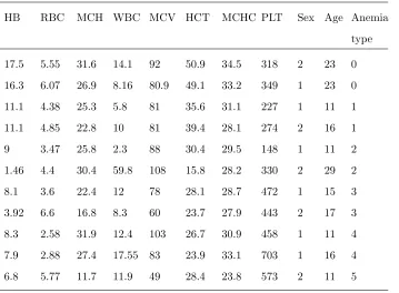
Table 1. Some samples from the data
HB RBC MCH WBC MCV HCT MCHC PLT Sex Age Anemia
type
17.5 5.55 31.6 14.1 92 50.9 34.5 318 2 23 0
16.3 6.07 26.9 8.16 80.9 49.1 33.2 349 1 23 0
11.1 4.38 25.3 5.8 81 35.6 31.1 227 1 11 1
11.1 4.85 22.8 10 81 39.4 28.1 274 2 16 1
9 3.47 25.8 2.3 88 30.4 29.5 148 1 11 2
1.46 4.4 30.4 59.8 108 15.8 28.2 330 2 29 2
8.1 3.6 22.4 12 78 28.1 28.7 472 1 15 3
3.92 6.6 16.8 8.3 60 23.7 27.9 443 2 17 3
8.3 2.58 31.9 12.4 103 26.7 30.9 458 1 11 4
7.9 2.88 27.4 17.55 83 23.9 33.1 703 1 16 4
6.8 5.77 11.7 11.9 49 28.4 23.8 573 2 11 5
2.2. Multiple Linear Regression Model. Consider a multiple linear regression (MLR) model with k
predictor variables, independent observations
y=B0+B1x1+B2x2+...+Bkxk+=B0+ k X
i=1
Bixi+. (2.1)
The observations recorded for each of thesenlevels can be expressed in the following way
y1=B0+B1x11+B2x12+...+Bkx1k+1
y2=B0+B1x21+B2x22+...+Bkx2k+2
.. .
yi=B0+B1xi1+B2xi2+...+Bkxik+i
.. .
yn=B0+B1xn1+B2xn2+...+Bkxnk+n
(2.2)
The dependent observationsy1, y2, ..., yn, and the independent observationsx1, x2
, ..., xk, haven levels. Thenxij represents the ith level of thejth predictor variable,xj.
System (2) can be represented as follows:
y= y1 y2 .. . yn
,X=
1 x11 x12 . . . x1k
1 x21 x22 . . . x2k
..
. ... ... ...
1 xn1 xn2 . . . xnk
,B=
B0 B1 .. . Bk , = 1 2 .. . n (2.4)
wherey,X,Bandstand for the observations, the regression coefficients and an unobserved random variable
that adds noise to the linear relationship between the dependent variable and regressors, respectively. To
obtain the regression model, B should be known. Therefore, B is estimated by using the least square
estimates as follows
ˆ
B= (XTX)−1XTy, (2.5)
whereXT represents the transpose of the matrixXwhile (XTX)−1represents inverse of the matrix (XTX).
Knowing the estimate ˆB, the MLR model can now be expressed as [33,34]
ˆ
y= ˆBX, (2.6)
where ˆyis the estimated value for yfrom the regression.
2.3. Test for the Model. The linear regression model estimation is selected and the sum of square tests.
The computation formula can be given as follows:
SST =
n X
j=1
(yj−y)¯ 2, SSR= n X
j=1
(ˆyj−y)¯ 2, SSE= n X
j=1
(yj−yˆj)2= n X
j=1
e2j. (2.7)
The coefficient of determination is a measure showing the rate of the contribution of the independent variables
in the interpretation of the change in the dependent variable as known from the literature [35,36]. It is given
as follow:
R2= SSR SST = 1−
SSE
SST. (2.8)
A terminological difference arises in the expression mean squared error (MSE). The MSE of a regression is a
measure of the average of the sum of squared error and how the concentration of data around the regression
model. The smaller the MSE, whenever the results are more accurate [35,36]. Then it is given by
M SE= 1 n
n X
j=1
e2j. (2.9)
3. Building Linear Regression Analysis Model
The currently produced MLR model is a linear equation determined as previously mentioned in Section
2.2. The obtained model is as follows:
y=B0+B1HB+B2RBC+B3M CH+B4W BC+B5M CV
+B6HCT+B7M CHC+B8P LT+B9Sex+B10Age+
whereyis type of the anemia andBi, 0≤i≤10, are the parameters to be determined.
The linear regression model, as explained in Section 2.2, is estimated as
ˆ
y= 6.377−0.224HB−0.224RBC−0.029M CH+ 0.001W BC
+0.0005M CV −0.016HCT+ 0.007M CHC+ 0.001P LT
−0.311Sex−0.009Age.
(3.2)
Here the coefficient values of the linear model have been obtained through the multiple regression approach,
to find the model that is more realistic (see Table 4). As previously mentioned, the model can be represented
in matrix form as follows:
ˆ
y= ˆBX (3.3)
where ˆ y= y1 y2 .. . y539
,X=
1 HB11 RBC12 . . . Age110
1 Hb21 RBC22 . . . Age210
..
. ... ... ...
1 HB539,1 RBC539,2 . . . Age539,10
,B=
6.377 −0.224 −0.224 −0.029 0.001 0.0005 −0.016 0.007 0.001 −0.311 −0.009 (3.4)
Here ˆy and X represent the estimates for output (types of the anemia) and the independent observations
matrix, respectively.
4. Results and Discussion
Different strategies of mathematical methods are implemented to analyze blood variables, as in the
lit-erature [16,18,22,37]. The multiple regression analysis have been taken into account by many researchers
[19,23-32] while dealing with various anemia problems at different levels. However, they used a limited
number of blood variables and they did not study a relationship for the prediction of the types of anemia.
Therefore, the current study concentrates on the investigation of the relationship between a very large
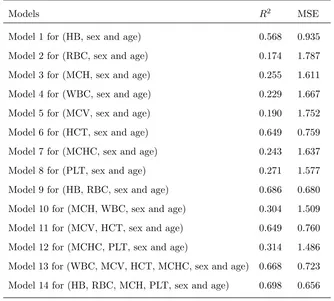
num-ber of blood variables and the types of anemia. Various versions of models, based on the variables, are
Table 2. Various forms of the multiple linear models: blood variables, sex, and age
Models R2 MSE
Model 1 for (HB, sex and age) 0.568 0.935
Model 2 for (RBC, sex and age) 0.174 1.787
Model 3 for (MCH, sex and age) 0.255 1.611
Model 4 for (WBC, sex and age) 0.229 1.667
Model 5 for (MCV, sex and age) 0.190 1.752
Model 6 for (HCT, sex and age) 0.649 0.759
Model 7 for (MCHC, sex and age) 0.243 1.637
Model 8 for (PLT, sex and age) 0.271 1.577
Model 9 for (HB, RBC, sex and age) 0.686 0.680
Model 10 for (MCH, WBC, sex and age) 0.304 1.509
Model 11 for (MCV, HCT, sex and age) 0.649 0.760
Model 12 for (MCHC, PLT, sex and age) 0.314 1.486
Model 13 for (WBC, MCV, HCT, MCHC, sex and age) 0.668 0.723
Model 14 for (HB, RBC, MCH, PLT, sex and age) 0.698 0.656
The models produced in terms of larger number of blood variables show better correlation than the models
produced in terms of less number of blood variables for predicting the types of anemia in equation (3.2).
However, naturally some of the variables are of more effect than others.
After the essential requirements have been verified for the multivariate analysis in equation (3.2), the
variables have been included for the MLR analysis. Those variables consist of regression coefficients B, the
blood variables (HB, RBC, MCH, WBC, MCV, HCT, MCHC, PLT), sex, and age. Therefore, the MLR
shows the synergistic effect of predicting the types of anemia better than the ones used fewer blood variables.
The enter method of the MLR has been used in the current analysis. All the variables were introduced into
the regression model as selected by the enter method of the MLR.
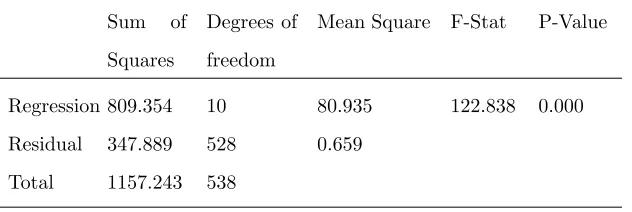
In the outcome of the current analysis, it has been found that there is a more significant relation
(R2=0.699) of the MLR model. It means that 69.90% of the change in the relationship between all blood
variables, sex, and age for the types of anemia is explained.
Thus, it is concluded that the regression model with the blood variables, sex, and age are seen to be
significant (p <0.000). That means simultaneous consideration of the blood variables, sex, and age has a
Table 3. Analysis of variance for the correlation in equation (3.2)
Sum of
Squares
Degrees of
freedom
Mean Square F-Stat P-Value
Regression 809.354 10 80.935 122.838 0.000
Residual 347.889 528 0.659
Total 1157.243 538
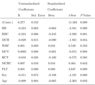
The standardized coefficient (Beta) compares the effect force of each individual blood variables, sex, and
age to the types of anemia. It is thus given byStandardizedBetaj=Bj∗SD(Xj)/SD(Y) .
The HB absolute value of the Beta coefficient is (−0.663) has the strongest relationship with the types of
the disease comparison to the other variables RBC (−0.345), Sex (−0.106), HCT (−0.100), MCH (−0.090),
PLT (0.080), Age (−0.065), WBC (0.016), MCHC (0.016) and MCV (−0.001). The interpretation of the
Beta value for the HB signifies that for every change in the HB, the dependent variable will be changed by
the Beta coefficient value (see Table 4).
Thet-test was used to measure the partial effect of the variables HB, RBC, MCH, WBC, MCV, HCT,
MCHC, PLT, sex, and age on the types of anemia. Notice that these variables have been seen to affect the
types of anemia but in varying rates (see Table 4). The histogram of the residuals which confirm that the
data are distributed according to a normal distribution with a mean of zero and a standard deviation of
0.991 (see Figure 1).
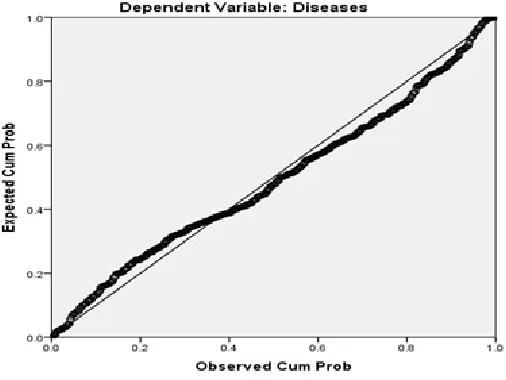
To find out the extent of spread the random error around the linear regression model, the MLR use the
mean square residuals, MSE=0.659 (see Table 3). Small values of the MSE indicate the concentration of
data around the linear regression model (see Figure 2).
In this study, comparing criteria are constructed on the principle of whether the technique provides a
suitable prediction or not. This task is achieved by comparing with the deep learning method (LSTM).
The results demonstrate that the linear regression has the best fit to the initial dataset comparing to the
deep learning method (LSTM) (see Table 5). Therefore, the present study provides an accurate model for
Table 4. Analysis of the multiple regression coefficients given in equation (3.2)
Unstandardized
Coefficients
Standardized
Coefficients
B Std. Error Beta t-Stat P-Value
(Const.) 6.377 0.552 11.563 0.000
HB -0.224 0.062 -0.663 -3.581 0.000
RBC -0.224 0.066 -0.345 -3.392 0.001
MCH -0.029 0.015 -0.090 -1.931 0.054
WBC 0.001 0.003 0.016 0.549 0.583
MCV 0.0005 0.008 -0.001 -0.015 0.988
HCT -0.016 0.028 -0.100 -0.575 0.565
MCHC 0.007 0.016 0.016 0.464 0.643
PLT 0.001 0.000 0.080 2.637 0.009
Sex -0.311 0.074 -0.106 -4.191 0.000
Age -0.009 0.004 -0.065 -2.303 0.022
Table 5. Comparison of the MLR results with the results of the linear deep learning method
Methods SSE MSE R2
Linear Regression Analysis 347.889 0.659 0.699
Linear Deep Learning Methods (LSTM) 349.869 0.665 0.695
LSTM: Long Short Term Memory
5. Conclusions and Recommendation
This study has forecasted the types of anemia through biomedical information under the consideration
of eight different blood variables, sex, and age of individuals. Multiple linear regression model, for the first
time, have been derived in forecasting the types of anemia. The results revealed that the regression model
is very promising and is capable of making the prediction. In the analysis of the current anemia problem,
the multiple regression method has been found to be more accurate than linear deep learning methods. It
has been concluded that the model is expected to be helpful for diagnosis of the types of anemia to health
providers and designing an appropriate treatment programs for their patients. For future research, these
Figure 1. Histogram plot of the residuals
Figure 2. Normal PP Plot of Regression Standardized Residual
References
[1] M. Farman, Z. Iqbal, A. Ahmad, A. Raza and EU. Haq, Numerical solution and analysis for acute and chronic Hepatitis B, Int. J. Anal. Appl. 16 (2018), 842-55.
[2] E. Gulbandilar, A. Cimbiz, M. Sari and H. Ozden, Relationship between skin resistance level and static balance in type II diabetic subjects, Diabetes Res. Clin. Pract. 82 (2008), 335-339.
[3] M. Sari, E. Gulbandilar and A. Cimbiz, Prediction of low back pain with two expert systems, J. Med. Syst. 36 (2012), 1523-1527.
[5] M. Sari, C. Tuna and S. Akogul, Prediction of tibial rotation pathologies using particle swarm optimization and K-Means algorithms, J. Clin. Med. 7 (2018), 65.
[6] S. Conoci, F. Rundo, S. Petralta and S. Battiato, In Advanced skin lesion discrimination pipeline for early melanoma cancer diagnosis towards PoC devices, 2017 European Conference on Circuit Theory and Design (ECCTD), 2017, IEEE, 1-4.
[7] M. Sari, Relationship between physical factors and tibial motion in healthy subjects: 2D and 3D analyses, Adv. Ther. 24 (2007), 772-783.
[8] M. Sari and BG. Cetiner, Predicting effect of physical factors on tibial motion using artificial neural networks, Expert Syst. Appl. 36 (2009), 9743-9746.
[9] C. Liddell, N. Owusu-Brackett and D. Wallace, A Mathematical model of sickle cell genome frequency in response to selective pressure from malaria, Bull. Math. Biol. 76 (2014), 2292-2305.
[10] M. Sari and C. Tuna, Prediction of pathological subjects using genetic algorithms, Comput. Math. Methods Med. 2018 (2018).
[11] World Health Organization. Worldwide Prevalence of Anaemia 1993-2005: WHO Global Database on Anaemia, 2008. [12] PC. Hbert, G. Wells, MA. Blajchman, J. Marshall, C. Martin, G. Pagliarello, M. Tweeddale, I. Schweitzer and E. Yetisir,
A multicenter, randomized, controlled clinical trial of transfusion requirements in critical care, N. Engl. J. Med. 340 (1999),409-417.
[13] A. Kim, S. Rivera, D. Shprung, D. Limbrick, V. Gabayan, E. Nemeth and T. Ganz, Mouse models of anemia of cancer, PLoS One 9 (2014), e93283.
[14] Li Xuejin, M. Dao, G. Lykotrafiti and GE. Karniadakis, Biomechanics and biorheology of red blood cells in sickle cell anemia, J. Biomech. 50 (2017), 34-41.
[15] J.C. McAllister, Modeling and control of hemoglobin for anemia management in chronic kidney disease, Doctoral Disser-tation, University of Alberta, 2017 (2017).
[16] N. Sirachainan, P. Iamsirirak, P. Charoenkwan, P. Kadegasem, P. Wongwerawattanakoon, W. Sasanakul, N. Chansatitporn and A. Chuansumrit, New mathematical formula for differentiating thalassemia trait and iron deficiency anemia in tha-lassemia prevalent area: a study in healthy school-age children, Southeast Asian J. Trop. Med. Public. Health. 45 (2014), 174-182.
[17] A. Ngwira and L. N. Kazembe, Analysis of severity of childhood anemia in Malawi: a Bayesian ordered categories model, Open Access Med. Stat. 6 (2016), 9-20.
[18] IL. Roth, B. Lachover, G. Koren, C. Levin, L. Zalman and A. Koren, Detection ofβ-thalassemia carriers by red cell parameters obtained from automatic counters using mathematical formulas, Mediterr. J. Hematol. Infect. Dis. 10 (2018), 1-10.
[19] F. Habyarimana, T. Zewotir and S. Ramroop, Structured additive quantile regression for assessing the determinants of childhood anemia in Rwanda, Int. J. Environ. Res. Public Health. 14 (2017), 652.
[20] S. Piplani, M. Madaan, R. Mannan, M. Manjari, T. Singh and M. Lalit, Evaluation of various discrimination indices in differentiating Iron deficiency anemia and Beta Thalassemia trait: A practical low cost solution, Ann. Pathol. Labor. Med. 3 (2016), A551-559.
[21] CV. Jimnez, Iron-deficiency anemia and thalassemia trait differentiated by simple hematological tests and serum iron concentrations, Clin. Chem. 39 (1993), 2271-2275.
[23] V. Sharma and R. Kumar, Dating of ballpoint pen writing inks via spectroscopic and multiple linear regression analysis: A novel approach, Microchem. J. 134 (2017), 104-113.
[24] X.Z. Huang, Y.C. Yang, Y. Chen, C.C. Wu, R.F. Lin, Z.N. Wang and X. Zhang, Preoperative anemia or low hemoglobin predicts poor prognosis in gastric cancer patients: a meta-analysis, Dis. Markers 2019 (2019), Article ID 7606128. [25] F. Al-Hadeethi and M. Al-Safadi, Using the multiple regression analysis with respect to ANOVA and 3D mapping to model
the actual performance of PEM (proton exchange membrane) fuel cell at various operating conditions, Energy, 90 (2015), 475-482.
[26] AM. Saviano and FR. Loureno, Measurement uncertainty estimation based on multiple regression analysis (MRA) and Monte Carlo (MC) simulationsApplication to agar diffusion method, Measurement, 115 (2018), 269-278.
[27] SM. Paras, A simple weather forecasting model using mathematical regression, Indian Res. J. Ext. Educ. 12 (2016), 161-168. [28] J. Daru, J. Zamora, B.M. Fernndez-Flix, J. Vogel, O.T. Oladapo, N. Morisaki, . Tunalp, M.R. Torloni, S. Mittal and K. Jayaratne, Risk of maternal mortality in women with severe anaemia during pregnancy and post partum: a multilevel analysis, Lancet Glob. Health, 6 (2018), e548-e554.
[29] Ho. Kok Hoe, P. Joshua and O. Kok Seng, A multiple regression analysis approach for mathematical model development in dynamic manufacturing system: a case study, J. Sci. Res. Develop. 2 (2015), 81-87.
[30] P.H. Nguyen, S. Scott, R. Avula, L.M. Tran and P. Menon, Trends and drivers of change in the prevalence of anaemia among 1 million women and children in India, 2006 to 2016, BMJ Glob. Health, 3 (2018), e001010.
[31] AJ. Prieto, A. Silva, J. de Brito, JM. Macas-Bernal and FJ. Alejandre, Multiple linear regression and fuzzy logic models applied to the functional service life prediction of cultural heritage, J. Cult. Herit. 27 (2017), 20-35.
[32] M. Little, C. Zivot, S. Humphries, W. Dodd, K. Patel and C. Dewey, Burden and determinants of anemia in a rural population in south India: A Cross-Sectional Study, Anemia 2018 (2018), Article ID 7123976.
[33] JO. Rawlings, SG. Pantula and DA. Dickey, Applied regression analysis: a research tool, Second Edition, Springer Science & Business Media, 2001.
[34] M. Srikanta and DG. Akhil, Chapter 4 Regression modeling and analysis, Applied Statistical Modeling and Data Analytics, A practical guide for the petroleum Geosciences, 1st Edition, Elsevier, (2018), 69-96.
[35] J.F. Rudolf, J.W. William and S. Ping, Regression analysis: statistical modeling of a response variable, Second Edition, Elsevier, 2006.
[36] AC. Cameron and PK. Trivedi, Regression analysis of count data, Cambridge University press, 2013.