Joint economic lot-sizing problem for a two-stage supply chain with price-sensitive demand

Sharif University of Technology

Transactions E: Industrial Engineering www.scientiairanica.com

Joint economic lot-sizing problem for a two-stage

supply chain with price-sensitive demand

M. Khojaste Sarakhsi, S.M.T. Fatemi Ghomi

_{and B. Karimi}

Department of Industrial Engineering, Amirkabir University of Technology, 424 Hafez Avenue, Tehran, Iran. Received 10 December 2014; received in revised form 4 May 2015; accepted 25 July 2015

KEYWORDS Joint economic lot-sizing problem; Price-sensitive demand;

Geometric shipment policy;

Geometric-then-equal size shipment policy; Optimal shipment policy.

Abstract. This paper studies Joint Economic Lot-Sizing problem (JELS) for a single-vendor single-buyer system while demand is dependent on selling price. This problem is modeled for geometric shipment policy and a solution procedure is developed to nd a well approximation of the global optimal solution of the problem. Since the equal-size shipment policy or geometric shipment policy may yield more joint prot compared to each other, the most important factor that aects the break-even point of geometric and equal-size policies is determined. The JELS problem for dependent demand is also modeled for geometric-then-equal size and optimal shipment policies. Solution procedures to nd a well approximation of the global optimum of each problem are also developed for these models. The models and solution procedures for geometric, geometric-then-equal size, and shipment policies are novel in the literature. Numerical results of the models show considerable improvement in the joint prot of the chain compared to lot-for-lot and equal-size shipment policies for chains with price-sensitive demand and it could be very interesting for supply chain coordinators and practitioners.

© 2016 Sharif University of Technology. All rights reserved.

1. Introduction

In today's competitive global market, companies are pushed towards not only integrating dierent decision processes within their operational borders, but also towards closely collaborating with their customers and suppliers [1]. Therefore, all parties need to seek Eco-nomic Order Quantity (EOQ) based on their integrated total cost function, rather than each party's individual cost functions. Such a problem is generally called Joint Economic Lot-sizing Problem [2]. A thorough review of the research dealing with coordinated vendor-buyer Supply Chain (SC) is gathered by Glock [3]. The Joint Economic Lot-Sizing problem (JELS) was developed in dierent aspects and focusing on shipment policies is one of the earliest attempts in this context.

*. Corresponding author. Tel.: +98 21 64545381; Fax: +98 21 66459569

E-mail address: [email protected] (S.M.T. Fatemi Ghomi)

The rst shipment policy studied in the JELS literature was lot-for-lot shipment policy (LP). In this policy, a production batch is shipped to the buyer as a single shipment. The rst study modeled total joint cost of a single-vendor single-buyer SC with innite production rate and was published in 1977 [4]. Then, this policy was developed by assuming nite production rate [5]. Kim et al. [6] also studied the LP for a system consisting of a manufacturer and a retailer with price-dependent demand while full coordination, partial coordination, and non-coordination mechanisms were applied to the system. Sana [7] adopted LP for a chain consisting of a manufacturer and a retailer while demand was dependent on the sale initiatives provided by the retailer.

The second shipment policy considered in the JELS literature was equal-size shipment policy (EP). In this policy, a production batch is divided to equal shipments. Two variants of EP are developed in the literature: delayed EP introduced by Goyal [8] and

non-delayed EP applied by Lu [9]. In the delayed EP, it is assumed that shipping the products from the vendor to the buyer is delayed until producing the entire production batch is nished. This assumption is relaxed in non-delayed EP and the rst shipment will be sent to the buyer when it is produced at the vendor. EP was investigated by Buscher and Lindner [10] for a production system with rework considerations. The focus of the paper is on the determination of production and rework lot sizes, but the optimal number of shipments is also determined by the proposed solution procedure. Total cost of an integrated two-stage system was optimized by Shu and Zhou [11] when vendor invested on setup cost reduction, process quality improvement, and EP as the shipment policy. Non-delayed EP was also studied for a three-layer vertically integrated SC involving a supplier, a manufacturer, and multi retailers with constant demand and increasing in-ventory holding costs in the downstream direction [12]. Abdelsalam and Elassal [13] extended the proposed model of [12] by applying stochastic demand while each retailer had its own holding and ordering costs that were not necessarily equal to those of other retailers. More examples of considering EP in the JELS problem optimization can be found in [14-16].

The third shipment policy was introduced in 1995 [17] that is known as geometric shipment policy (GP). In this policy, a growth factor that is equal to the ratio of production rate to demand rate, p

D, is

applied to the size of shipments. Therefore, if size of the rst shipment is named q1, the nth shipment

size will be equal to q1 _Dpn 1. Later, Hill [18]

assumed the growth factor as a decision variable and developed a solution procedure to nd a locally optimal solution of the resultant problem. GP with a constant growth factor has recently been considered, in which the production of defective items has been taken into account and the manufacturer should pay a warranty cost for each identied defective product [19].

The fourth shipment policy in the JELS literature is known as Geometric-then-Equal size Policy (GEP). First, Goyal and Nebebe [20] considered the ratio of the rst shipment to the remaining equal shipments equal to p

D. So they considered:

q1; q1_Dp; q1_Dp; q1_Dp; :::

as the size of shipments.

Later, Ben-Daya et al. [1] generalized the pro-posed policy of [20], considering that the rst m shipments followed the geometric policy and the size of equal shipments was similar to that of the last geometric shipment.

Hill [21] developed a new shipment policy as the result of relaxing the assumption of predetermined shipment policy using Lagrangian multiplier. He

proved that the developed policy, named Optimal Policy (OP), is similar to GEP, but the size of n m equal shipments is not necessarily equal to the size of the last geometric shipment. He also developed a solution procedure to solve the joint cost model of the chain.

Integrating pricing decision with ordering, in-ventory, and shipment decisions is another stream of research in JELS literature. Whitin [22] was the rst one who modeled EOQ for price-sensitive demand for an SC in 1995. This stream was continued by Jokar and Sajadieh [23]. They optimized total joint prot of an SC by integrating ordering, shipment, and pricing policies considering LP as shipment policy and price-dependent demand. Another eort to optimize joint prot of a chain with price-sensitive demand while EP is applied can be found in [24]. Joint-pricing and lot-sizing policies for price-dependent demand was investigated by Kim et al. [25] for a system while LP was adopted for shipment of the products. In another study, Huang et al. [26] tried to coordinate pricing and inventory decisions for a three-stage SC consisting of multiple suppliers, single manufacturer, and multiple retailers as a non-corporative game. More examples of recent research in this area can be found in [27-29]. The JELS problem was also modeled for price and environmentally dependent demand when EP was adopted [30]. Joint-pricing and lot-sizing problem for a two-stage system was studied by Ghasemy Yaghin et al. [31] when supplier followed EP and demand was price-sensitive through a logit function with a price discount for the orders arrived prior to the sale period. A two-stage system was also investigated for a multi-product chain where demand for each multi-product at each retailer was dependent on its price, price of other com-petitors, and the price of substitutable products [32]. As another eort to integrate lot-sizing and pricing policies, Taleizadeh and Noori-daryan [33] modeled a three-stage SC to nd the minimum total cost of the chain using Stackelberg-Nash equilibrium to optimize the cost incurred by the members. Wang et al. [34] also modeled the JELS problem for price-dependent demand with innite production rate. They considered both linear and non-linear dependency functions and solved the corresponding models for centralized and decentralized conditions.

Besides the extensions focusing on the various shipment policies and eorts to integrate joint-pricing and lot-sizing policies, the JELS problem was also extended by other considerations. Integrated vendor-buyer model with stock-dependent demand was studied for coordinated and non-coordinated SCs [35]. Three-stage SC with imperfect quality products was consid-ered by Sanaz [36] while assuming production rate as a decision variable and dierent probability distribu-tion funcdistribu-tions for defective items. Lee and Fu [37]

investigated a make-to-order two-echelon SC while considering transportation cost between the vendor and the buyer.

To the best of our knowledge, joint lot-sizing and pricing is only studied for LP and EP and there is no research considering it for neither GP, nor GEP, nor OP. To ll this gap, we model the joint prot of a two-stage SC for these shipment policies and develop their corresponding solution procedures to nd the optimal solutions. Besides, as for some problem instances, total prot obtained by adopting EP is greater than that of GP and vice versa. Also, there is no analysis comparing optimal prots of EP and GP; we compare their optimal joint prots for price-sensitive demand and nd the most important factor that aects break-even point of them.

The main contributions of this paper can be summarized as follows. First, for the joint prot model of GP, the paper determines the upper and the lower limits for the number of shipments and develops a search based procedure to nd the optimal solution. Second, it determines the break-even point of EP and GP for price-dependent demand. Third, similar to GP, the optimal solution for the joint prot model is determined. Fourth, for OP, the optimal selling price, production batch size, and the number of shipments are obtained by the proposed solution procedure.

In all of the developed solution procedures, secant method is used to determine a well approximation of the global optimum. Convergence properties of the secant method are studied in some research like [38-39]. In the current paper, the performance of the proposed procedure is evaluated by comparison of its optimal solution with the optimal solution obtained by adopting a Simulated Annealing (SA) algorithm.

This paper is organized as follows. Section 2 denes the general JELS problem and its assumptions. In section 3, the JELS problem with GP is modeled and a solution procedure is developed to nd the optimal solution of the model. Section 4 investigates the optimal solutions of the proposed procedure and the SA algorithm. Section 5 gives a comparison of EP and GP and also determines break-even point of these policies. Section 6 deals with the JELS problem for GEP. Section 7 models the JELS problem when OP is applied to the chain and develops its optimal solution procedure. Section 8 presents numerical results and sensitivity analysis of the problem parameters. Finally, Section 9 is devoted to the conclusions and recommen-dations for future research.

2. Problem denition and assumptions

This paper studies a single-vendor single-buyer SC of a single product. Similar to other research in the JELS

literature, time horizon is assumed to be innite, and shortage is not allowed. In addition, production rate is assumed to be nite and greater than the demand rate. The demand (D) for the nal product is linearly dependent on selling price (). The dependency function is D() = a b. The buyer's inventory holding cost is greater than that of the vendor, and the buyer continuously reviews its inventory. The following notations are used in the paper:

P Vendor's production rate;

D Demand rate as a function of selling price;

Buyer unit selling price (paid by nal customer);

Av Vendor's setup cost;

Ab Buyer's ordering cost;

hv Vendor's inventory holding cost per

year per unit product;

hb Buyer's inventory holding cost per year

per unit product; n Number of shipments;

m Number of equal shipments in a cycle; l Geometric growth factor (p=D); Q Vendor production batch size;

q1 First shipment size from the vendor to

the buyer.

The JELS model has a general formulation as shown in Eq. (1). The objective of this model is to minimize total cost of the chain and it consists of ordering and inventory holding costs of the chain's members:

TCjoint= (Av+ NA_Q b)D+ hvIs+ (hb hv)Ib; (1)

where:

Is= q1D_p + Q(p D)_2p ; (2)

Ib=

PPP_n

1q2i

2Q : (3)

3. Geometric shipment policy (GP)

The idea of GP was rst introduced in 1995 [17]. In this policy, the size of each shipment is a multiplier of the rst shipment size as presented in Eq. (4). The production batch size is equal to the sum of shipments in a cycle; its corresponding expression is shown in Eq. (5):

The size of the rst shipment can be written as Eq. (6): Q = q1(ln 1)

l 1 ; (5)

q1=Q(l 1)_{ln 1} : (6)

The objective of the general JELS model is to minimize total joint cost of the chain, but the current paper maximizes the total joint prot of the chain. Therefore, the exchange price between the vendor and the buyer has no eect on the joint prot of the chain. Here, the chain revenue is achieved through selling the nal products to the customers, D, that can be rewritten as D(a D)_b . By replacing inventories of the system and the buyer in the general JELS model, total joint prot of the chain for GP becomes as Eq. (7). Since this expression is concave in q1, the optimal value of

this variable, q

1, can be determined using the rst

derivative of the joint prot relative to q1, as shown

in Eq. (8): T OGP

joint(q1; D; n) =D(a D)_b

(Av+ nAb)

p D D D q1

pn _Dn

Dn hv 2 4D p +

(p D)pn_DnDn

2pp D_D

3 5 q1

(hb hv)

2 4 (p

n _Dn₎

Dn

2p+D_D 3

5 q1; (7)

q 1GP = v u u u u u t

(Av+nAb)(p DD )D

(pn Dn Dn )

hv

D p +

(p D)(pn Dn Dn )

2p(p D D )

+(hb hv)

(pn+Dn

Dn )

2(p+D D )

: (8) By replacing the optimal value of q1in T PjointGP (q1; D; n)

and after some manipulation, the total joint prot of the chain becomes as Eq. (9). Constraints of this model are shown in Relations (10) and (11):

T PGP

joint(D; n) = D(a D)_b

2 s

(Av+ nAb)D(Dhv+ phb)(pn+ Dn)(p D)

2p(pn _Dn_{)(p + D)} ;

(9)

D 0; (10)

n : integer: (11)

Since there is no closed form for optimal D or n that can be determined by the corresponding rst and second derivatives, the remaining analysis to nd the optimal values of these variables should be continued based on the numerical methods.

As n is an integer variable, it is of great interest to determine its upper and lower limits and then search through the interval of these limits for optimal D. To nd these limits, the objective function can be rewritten as a function of n as shown in Eq. (12):

T P0GP joint(n) =

s

(Av+ nAb)(pn+ Dn)

(pn _Dn₎ : (12)

The rst derivative of the above expression relative to n is as follows:

@T P0GP joint(n)

@n =

Ab(p2n D2n) 2pnDn(Av+nAb)(log(p) log(D))

2(pn _Dn₎p_(Av+nAb)(p2n _D2n₎ :

(13) As a

b, D belongs to (0; a). On the other hand p >

D, therefore @T P0GPjoint(n)

@n is always less than zero and

consequently T P0GP

joint(n) is a non-increasing function

of D. Therefore, the upper and the lower limits of n can be found by the following two procedures:

- Procedure 1: Find the upper limit of n (nGP max)

(a) Replace D with its lower limit, zero, in T PGP

joint(D; n);

(b) Determine the optimal n that maximizes T PGP joint

(D = 0; n) using Secant method [39];

(c) The ceiling of the resultant n is the upper limit of this variable (nGP

max).

- Procedure 2: Find the lower limit of n (nGP min)

(a) Replace D with its upper limit, a, in T PGP joint(D; n);

(b) Determine optimal n that maximizes T PGP joint(D =

a; n) using Secant method;

(c) The oor of the resultant n is the lower limit of this variable (nGP

min).

Solution procedure

The following procedure is developed to solve the model.

- Step 1. Calculate nGP

min and nGPmax;

- Step 2. Set T PGP

opt and n = nGPmin;

- Step 3. Determine D that maximizes T PGP joint(D; n)

using Secant method and save the corresponding objective function value;

- Step 4. If T PGP

joint(D; n) > T PoptGP, then set nopt= n,

T PGP

- Step 5. Increase n by 1.;

- Step 6. If n < nGP

max, go to Step 3; otherwise, go to

Step 7;

- Step 7. The current solution is optimal. 4. Investigate performance of the proposed

procedure vs. Simulated Annealing (SA) algorithm

To study the performance of the proposed procedure in Section 3, we solve the JELS problem for GP by implementing a Simulated Annealing (SA) algorithm. SA is a powerful algorithm commonly used for heuristic optimization due to its simplicity and eectiveness. Within this approach, variables to be optimized are viewed as the degrees of freedom of a physical system and the cost function of the optimization problem as the energy [40]. We implement an SA algorithm while the optimal solution obtained by the proposed proce-dure is considered as the initial solution to start the SA algorithm. The steps of the customized and tuned SA algorithm to solve the JELS problem are as follows. To reduce run time and enhance the performance of the SA algorithm, the maximum number of neigh-bors is linearly dependent on the temperature; more neighbors are generated for high temperatures, and as temperature decreases, less neighbors are considered to accelerate the convergence process.

- Step 1. Set the optimal solution of the proposed procedure as the initial solution and its objective function value as Zopt;

- Step 2. Set initial temperature (t) = 100 and nal temperature = 10 200_;

- Step 3. While t < 10 200_:

3.1. Set maximum number of neighbors (nmax) as

70t;

3.2. While number of neighbors is less than nmax:

3.2.1 Randomly select between neighborhood generation methods A and B:

A. Assign a random number to one of the variables regarding its con-straint;

B. Swap values of two variables regard-ing their constraints.

3.2.2. Calculate objective function of the neighbors (Z);

3.2.3. If Z > Zopt, update the optimal

so-lution found so far and increase num-ber of neighbors by one. Otherwise, calculate acceptance probability, p =

Z Z opt

t . Generate a random number;

if p is greater than it, increase number of neighbors by one.

3.3. Set the best solution found in this t as optimal and its objective function value as Zopt;

3.4. Schedule cooling by updating temperature as 0:9t.

- Step 4. The best solution obtained in all tem-peratures is the optimal solution. The comparison between the optimal joint prots of the SA algorithm and the proposed procedure is shown in Table 1 for the benchmark problem of the JELS literature. The parameters of this problem are as follows:

p = 3200=year; hv = $4=unit=year;

hb = $5=unit=year Av = $400=setup;

Ab= $25=setup; a = 1500; b = 50:

As presented in the table, for 10 runs of the algorithms, there is just a small dierence between their optimal prots. Therefore, we can claim that

Table 1. Comparison of optimal prots obtained by the SA algorithm and the proposed procedure. Run # Optimal prot

obtained by SA

Optimal prot obtained by the proposed procedure

% dierence in optimal prot 1 9,617.502511572 9,617.519119639 0.000172686 2 9,617.504099580 9,617.519705279 0.000162263 3 9,617.517440652 9,617.519798804 0.000024519 4 9,617.507101522 9,617.518986796 0.000123579 5 9,617.513974360 9,617.518703130 0.000049168 6 9,617.519540566 9,617.519799290 0.000002690 7 9,617.513821152 9,617.519181529 0.000055736 8 9,617.519625431 9,617.519790744 0.000001719 9 9,617.508403004 9,617.519788001 0.000118378 10 9,617.513707257 9,617.519779509 0.000063137

the proposed procedure to solve the JELS problem has a good performance and its solution is a well approximation of the global optimum of the problem. It should be notied that the proposed algorithm is preferred due to its short run time compared to the SA algorithm while its performance is approximately the same. Besides, the proposed procedure uses secant method that is a traditional method and it can be easily implemented.

5. Comparison of equal shipment policy with geometric shipment policy

In the EP, all the orders are equal; so ordering and shipment management of this policy is simple for partners. On the other hand, in GP, the size of orders increases geometrically; so the time between two orders and the transportation capacities should be altered for each order. The main concentration of EP besides the simplicity of management is to minimize average inventory of the buyer while the main concentration of GP is to minimize the vendor's average inventory. These facts are presented in Figures 1 and 2 for the benchmark problem of the JELS literature for dierent values of the buyer's inventory holding cost near its value in the benchmark problem.

Therefore, it seems that the inventory holding cost of the vendor and the buyer may aect the eciency of these two policies. To study this issue, the benchmark problem of JELS literature is considered.

Figure 3 illustrates the eect of hb=hvon the total

joint prot of the chain. It can be inferred from the gure that there is a Break-Even Point (BEP) of EP and GP. Analyzing sensitivity of the total joint prot to other parameters of the problem and determining the BEP for some problem instances based on all parame-ters conrm the major eect of inventory holding cost

Figure 1. Eect of buyer's inventory holding cost on buyer's inventory.

Figure 2. Eect of buyer's inventory holding cost on vendor's inventory.

Figure 3. Eect of hb=hvon the total joint prot.

on the BEP of EP and GP. Indeed, when the range of parameters of a problem does not thoroughly change, as in practice happens, the main factor that aects this point is the ratio of hb to hv. When this ratio is

greater than BEP, less inventory of buyer is desired, so EP shows better performance; but when this ratio is less than BEP, less inventory of vendor is desired, so GP is preferred. As shown in Figure 3, the value of hb=hv at the BEP of the benchmark problem is equal

to 1.37. Therefore, when hv = 4, if hb is smaller than

5.48, GP shows better performance; otherwise, EP is preferable. Determination of this point can be helpful when the chain coordinator decides to choose between EP and GP. The BEP can be determined using the interpolation method to nd the ratio of hb to hv.

6. Geometric-then-equal size shipment policy (GEP)

As explained in Section 5, EP or GP may yield more joint prot compared to each other. Therefore,

it is of great interest to combine these policies and simultaneously benet from their advantages. Ben-Daya et al. [1] generalize the proposed policy of [20] called geometric-then-equal size shipment policy. The size of shipments in this combined policy is according to Eq. (14):

qi=

( li 1 _q

1 i = 2; 3; :::; m

lm 1 _{q1 i = m + 1; :::; n} (14)

Based on the shipments' size, the production batch size is shown in Eq. (15).

Q = m X i=1 p D _{i 1}

q1+ (n m) p_D

_{m 1} q1

= q1

2 4

pm _Dm

Dm

p D D

+ (n m)

p D

m 13₅

= q1'q(D; m; n): (15)

The average inventories of the system and the buyer are also obtained as follows:

Is=

2 6 6 6 4 D p+ (p D) _{pm Dm} Dm p D

D +(n m)

p D _{m 1} 2p 3 7 7 7 5q1

= q1's(D; m; n); (16)

Ib=q₂1

2 4

p2m _D2m

D2m +(n m) _Dp

2m 2p2 _D2

D2 p+D D h

pm _Dm

Dm

+(n m) p D

m 1_{p D} D

i 3 5

= q1'b(D; m; n): (17)

Using the above expressions, the total joint prot of the chain for GEP is presented in Eq. (18). Again, this equation is concave in q1 and by a similar analysis, the

optimal value of this variable is as Eq. (19) and the modied objective function with its 3 variables is show in Eq. (20). It should be notied that 1 m n.

T PGEP

joint(q1; D; m; n) = D(a D)_{b q}(Av+ nAb)D 1'q(D; m; n)

hvq1's(D; m; n) (hb

hv)q1'b(D; m; n); (18)

q 1GEP=

s

(Av+nAb)D

'q(D;m;n)[hv's(D;m;n)+(hb hv)'b(D;m;n)] (19)

T PGEP

joint(D; m; n) = D(a D)_b 2

s

(Av+nAb)D

'q(D; m; n)[hv's(D; m; n)+(hb hv)'b(D; m; n)]₍₂₀₎

Similar to GP, determining the upper and the lower limits of n can be useful here. Since GEP is a combination of GP and EP, nding the upper and the lower limits of n is straightforward. According to [24], the lower and the upper limits of n for EP are as Eqs. (21) and (22), respectively;

nEP

min= max

8 < :

s

Av(hb hv)

Abhv ; 1

9 =

;; (21)

nEP max=

s

Avp(hb hv) + 2hvAva

Abhv(p a) : (22)

Since the optimal value of n is not out of the range of this variable in its parent policies, GP and EP, the limits of n in GEP, are as Eqs. (23) and (24).

nGEP min = min

nEP

min; nGPmin ; (23)

nGEP max = max

nEP

max; nGPmax : (24)

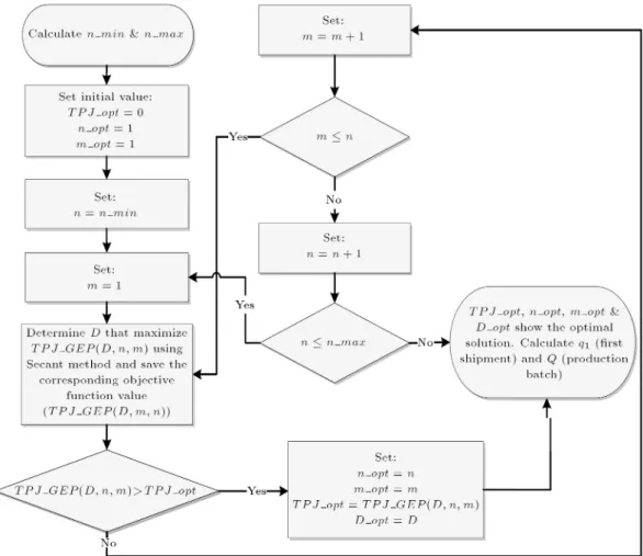
To nd the optimal values of variables with respect to the constraints, the following algorithm depicted in Figure 4 is developed. The proposed procedure to solve the model is similar to what was developed for GP as shown in Figure 4. According to Section 4, the nal solution is a well approximation of the global optimal solution.

7. Optimal shipment policy (OP)

The last shipment policy introduced in the JELS literature is OP. The size of shipments in this policy is very similar to that in GEP. Using Lagrangian multipliers recursively, Hill [41] introduced this policy with the following size of shipments:

qi =

( li 1 _q

1 i = 1; 2; :::; m Q Pm

i=1qi

n m i = m + 1; :::; n

(25) Hill [41] denes c as hv

hb hv and shows that if there

is no positive integer m < n, for which the following constraint holds, the OP changes to GP. By careful checking of this constraint, we found that there was a mistake in his expression. In other words, when we tried to obtain the constraint showed in Eq. (26) using the steps explained in [41], the resultant constraint was dierent. Further eorts ensured us that the

Figure 4. Solution procedure for JELS model when geometric-then-equal size shipment policy is applied.

correct constraint was as Eq. (27); therefore, we use this equation in the remaining analysis:

c _{(n m)(l 1)}l(lm 1) +l

(l2m ₁₎

(l2 ₁₎ + (l m ₁₎2

(n m)(l 1)2

(n m)lm₊lm ₁

l 1

; (26) c l(lm 1)

(n m)(l 1)

l(l_(l2m2 ₁₎1)+ (l m ₁₎2

(n m)(l 1)2

(n m)lm₊lm ₁

l 1

= (D; m; n): (27)

It should be notied that l in the above constraint is equal to p

D and can be replaced with this value.

According to [41], we can rewrite the size of the rst shipment as shown in Eq. (28). In a similar way, average inventories of the system and the buyer are presented in Eqs. (29) and (30), respectively:

q1= Q

_{pm Dm}

Dm

(n m)(p D D )

cD p _{p2m D2m}

D2m

p2 D2 D2

_{+ (}pm DmDm ) 2

(n m)(p D D )2

= Qq(D; m; n);

(28)

Is=

q(D; m; n)D

p +

(p D) 2p

Q = Qs(D; m; n);

(29)

Ib=

2 6 6 6 4

p2m D2m D2m

(n m)p2 D2 D2

₊cD_p 2

2

p2m D2m D2m

_{p2 D2}

D2

_{+ (}pm DmDm )2

(n m)(p D D )2

3 7 7 7 5Q

= Qb(D; m; n): (30)

Here, size of the production batch is considered as a decision variable and again the total joint prot is concave in Q. Therefore, the optimal production batch size, Q

OP, and modied objective function are

presented in Eqs. (32) and (33): T POP

joint(Q; D; m; n) = D(a D)_b (Av+ nA_Q b)D

hvQs(D; m; n) (hb hv)Qb(D; m; n);

(31) Q

OP =

s

(Av+ nAb)D

Figure 5. Solution procedure for JELS model when optimal shipment policy is applied.

T POP

joint(D; m; n) =D(a D)_b

2p(Av+nAb)D[hvs(D; m; n)+(hb hv)b(D; m; n)]:

(33) As stated in [41], the minimum total cost of the chain is achieved when hb= hv. In this condition, the objective

function becomes minimization of the total stock in the system and this was used to determine the maximum number of shipments, n.

There are two dierences between the objective functions of the current paper and the model consid-ered in [41]. First, the objective of our model is to maximize the total prot of the chain while minimizing total cost is the objective of [41]; second, since we consider D as a decision variable, the current paper has a further variable compared to the model studied in [41]. In the current paper, the upper limit of the total joint prot is obtained by considering hb hv and

it can be used to nd the upper limit of n as presented in Eq. (34):

T POP

limit(D; m; n) = D(a D)_b

2p(Av+ nAb)Dhvs(D; m; n): (34)

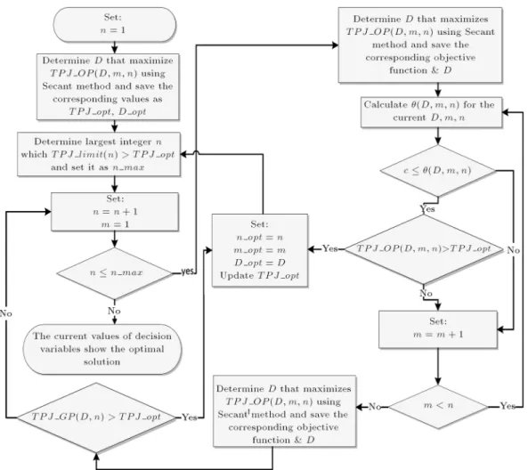
The solution procedure for the joint prot of the chain when applying OP is depicted in Figure 5. As shown, if there is no integer m < n that can pass the constraint, the objective function of GP will be applied that is referred to in the gure as T P J GP (D; n). Again, according to Section 4, the nal solution is a well approximation of the global optimal solution of the problem.

8. Numerical results and sensitivity analysis To analyze and compare all the shipment policies intro-duced in the literature for price-sensitive demand, we rst implement the solution algorithm of the equal-size policy introduced by Sajadieh and Akbari Jokar [24] in Matlab Software. Comparison of the results of the implemented algorithm with numerical results of [24] conrmed the validity of this implementation. In the current paper, GP, GEP, and OP are studied for dependent demand.

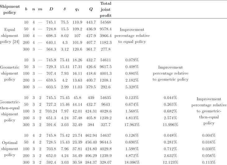
The eect of dierent values of b on the optimal solution of the benchmark problem is shown in Table 2

Table 2. Optimal solutions of equal, geometric, and geometric-then-equal shipment policies. Shipment

policy b n m D q1 Q

Total joint prot Equal

shipment policy [24]

10 4 | 745.1 75.5 110.9 443.7 54568

Improvement percentage relative

to equal policy 50 4 | 724.8 15.5 109.2 436.9 9578.4

100 4 | 698.3 8.02 107 427.9 3966.4 200 4 | 640.1 4.3 101.9 407.7 1182.3 300 3 | 564.3 3.12 120.6 361.7 277.8

Geometric shipment

policy

10 3 | 745.9 75.41 18.26 432.7 54611 0.079%

Improvement percentage relative to geometric policy 50 3 | 729.3 15.41 17.31 426.6 9617.5 0.408%

100 3 | 707.4 7.93 16.11 418.6 4001.3 0.880% 200 3 | 659.5 4.2 13.63 400.7 1208.1 2.182% 300 3 | 603.5 2.99 11.03 379.5 292.6 5.328%

Geometric-then-equal shipment

policy

10 3 2 745.5 75.45 45.8 439 54635 0.123% 0.044% _Improvement

percentage relative to

geometric-then-equal policy 50 3 2 727.2 15.46 44.14 432.7 9643 0.674% 0.265%

100 3 2 703.24 7.97 42.01 424.31 4028.6 1.568% 0.682% 200 3 2 651.3 4.24 37.48 405.8 1239.2 4.813% 2.574% 300 3 2 591.6 3.03 32.49 384 327.7 17.963% 11.996%

Optimal shipment

policy

10 4 2 745.8 75.42 23.74 462.94 54637 0.126% 0.048% 0.004% 50 4 2 728.5 15.43 23.39 456.40 9644.5 0.690% 0.281% 0.016% 100 3 2 703.8 7.96 37.81 424.80 4029.8 1.598% 0.712% 0.030% 200 3 2 652.0 4.24 34.49 406.29 1239.9 4.872% 2.632% 0.056% 300 3 2 592.4 3.03 30.58 384.37 328.07 18.096% 12.123% 0.113%

for all shipment policies. As the ratio of hbto hvfor this

problem is smaller than this ratio in the corresponding BEP, it is expected that GP yields more joint prot than EP.

According to the denition of b, as this parameter increases, dependency of the demand on the selling price increases. Therefore, determining the optimal selling price is of great importance. According to Table 2, as b increases, the total joint prot of the chain deceases. A part of this decrease can be compensated by using OP instead of the other policies. Using GEP also yields more joint prot than its parents' policies. For example, when b = 300, if the chain coordinator applies GEP instead of EP, the total joint prot increases by 17.96%; The resultant prot improvement of applying OP instead of EP also increases by 18.09%. These improvements can be very interesting for SC members, especially for centralized chains as the chain coordinator can decide how to ship the products be-tween the chain members.

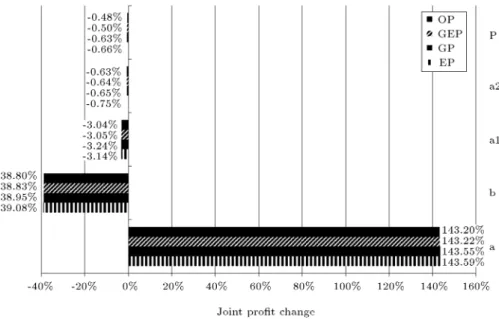
Figure 6 illustrates the eect of 50% increase in the value of a; b; a1; a2, and p for the benchmark

problem. The eect of hb and hv on the joint prot

was previously studied in Section 9.

As expected, among these parameters, a has the most impact and p has the least impact on the joint prot of the policies. Since a is the potential demand of a product, it has major inuence on the joint prot; but it is benecial to study the eect of b on the objective function value. Figure 7 depicts the eect of dierent values of b on the optimal prot of the chain for four shipment policies. The exponentially decreasing behavior of the joint prot is similar for the policies. The behavior can be explained by considerable reduction in actual demand, a b, as sensitivity to the selling price, b, increases slowly.

9. Conclusion and recommendations for future studies

This paper analyzed the Joint Economic Lot-Sizing (JELS) model for a two-stage supply chain while demand for the nal product was linearly dependent on the selling price. The main contributions of this paper can be summarized as follows. First, for the joint prot model of geometric shipment policy (GP), it determines the upper and the lower limits for the number of shipments and develops a search based algorithm to

Figure 6. Joint prot change for 50% increase in the values of parameters.

Figure 7. Eect of b on joint prot of shipment policies.

nd the optimal solution. Second, it determines the break-even point of equal-size shipment policy (EP) and GP for price-dependent demand. Third, similar to GP, the optimal solution for the joint prot model is determined. Fourth, for optimal shipment policy (OP), the optimal selling price, production batch size, and the number of shipments are obtained by the proposed solution procedure. In all of the developed solution procedures, secant method was used to determine a well approximation of the global optimal solution. The performance of the proposed procedure was also veried by investigating its optimal solution vs. the one obtained by the simulated annealing algorithm.

To explain the second contribution of the paper, it should be notied that comparison of the optimal solu-tions of EP and GP for dierent instances proved that choosing the best policy between them was dependent on the parameters' values of the problem. As shown in the paper, when the range of parameters does not

thoroughly change, as in practice happens, the ratio of vendor's inventory holding cost to buyer's inventory holding cost is the most important factor aecting Break-Even Point (BEP) of these two policies. When this ratio is greater than BEP, less buyer inventory is desired, so EP has better performance than GP; but when this ratio is less than BEP, less vendor inventory is desired, so GP is preferred. To determine this point, an interpolation method was applied.

Sensitivity analysis of the problem's parameters conrmed the major eect of demand dependency function on the joint prot of the chain. The analysis also showed an exponentially decreasing behavior of the joint prot as the slope of demand function (b) increased. Therefore, optimal solutions of the joint model were studied for dierent values of b. Numer-ical results suggest when demand is price-sensitive, applying OP, GEP, and GP, respectively, yields more joint prot than EP. Numerical results also proved that as b increased, more improvement would be achieved compared to EP. As an example, if the vendor ships the products to the buyer according to OP, the total joint prot of the chain for the benchmark problem of the JELS literature increases by 18.096% compared to EP when b = 300. From the managerial insight for products with high demand dependency on selling price, selecting GP, GEP, or OP instead of adopting lot-for-lot or equal shipment policies can signicantly increase the joint prot of the chain. It should be no-tied that achieving such a percentage of improvement by changing the shipment policy is straightforward and does not need any more investment; it just needs a good planning for shipments, while implementing other ideas to increase joint prot is not simple or needs considerable investment, such as investing in advertise-ment to aect the parameters of demand dependency

function. This signicant prot improvement can be very interesting for supply chain coordinators as well as the chain members, especially in centralized chains that the joint prot is the main aim of all the members. When adopting GP, GEP, or OP for the chain, various sizes of shipments make the implementation of these policies dicult and need a good planning and cooperation between the chain members to uti-lize its more joint prot. On the other hand, if we want to apply these policies for non-coordinated supply chains, developing incentives and prot sharing mechanisms are needed to persuade the members for joint commitment to implement these policies. In this study, the geometric growth factor considered in GP, GEP, and OP is equal to production rate to demand rate. Assuming it as a decision variable would be interesting for future research. Studying non-linear dependency of the demand on the selling price could be interesting for more research. Considering imperfect quality of the products and adding capacity constraint of the transportation equipment to the model is recommended for future studies. Integrating inbound logistics of the vendor to the JELS model and optimizing its corresponding costs are other areas for future researches. Investigating more retailers by equal or dierent ordering cycles and dierent demand rates are also recommended for more research.

Acknowledgment

The authors would like to thank Dr. M.S. Sajadieh for his helpful comments and suggestions.

References

1. Ben-Daya, M., Darwish, M. and Ertogral, K. \The joint economic lot sizing problem: Review and ex-tensions", European Journal of Operational Research, 185(2), pp. 726-742 (2008).

2. Sari, D.P., Rusdiansyah, A. and Huang, L. \Models of joint economic lot-sizing problem with time-based temporary price discounts", International Journal of Production Economics, 139(1), pp. 145-154 (2012).

3. Glock, C.H. \The joint economic lot size problem: A review", International Journal of Production Eco-nomics, 135(2), pp. 671-686 (2012).

4. Goyal, S.K. \An integrated inventory model for a single supplier-single customer problem", International Journal of Production Research, 15(1), pp. 107-111 (1977).

5. Banerjee, A. \A joint economic lot-size mode for purchaser and vendor", Decision Sciences, 17(3), pp. 292-311 (1986).

6. Kim, J., Hong, Y. and Kim, T. \Pricing and ordering policies for price-dependent demand in a supply chain

of a single retailer and a single manufacturer", Inter-national Journal of Systems Science, 42(1), pp. 81-89 (2011).

7. Sana, S.S. \Optimal production lot size and reorder point of a two-stage supply chain while random de-mand is sensitive with sales teams' initiatives", Inter-national Journal of Systems Science, 47(2), pp. 450-465 (2016).

8. Goyal, S.K. \`A joint economic-lot-size model for pur-chaser and vendor': A comment", Decision Sciences, 19(1), pp. 236-241 (1988).

9. Lu, L. \A one-vendor multi-buyer integrated inventory model", European Journal of Operational Research, 81, pp. 312-323 (1995).

10. Buscher, U. and Lindner, G. \Optimizing a production system with rework and equal sized batch shipments", Computers & Operations Research, 34(2), pp. 515-535 (2007).

11. Shu, H. and Zhou, X. \An optimal policy for a single-vendor and a single-buyer integrated system with setup cost reduction and process-quality improvement", In-ternational Journal of Systems Science, 45(5), pp. 1242-1252 (2013).

12. Ben-Daya, M., As'ad, R. and Seliaman, M. \An integrated production inventory model with raw ma-terial replenishment considerations in a three layer supply chain", International Journal of Production Economics, 143(1), pp. 53-61 (2013).

13. Abdelsalam, H.M. and Elassal, M.M. \Joint economic lot sizing problem for a three-Layer supply chain with stochastic demand", International Journal of Production Economics, 155, pp. 272-283 (2014).

14. Ho, W.T. and Hsiao, Y.C. \An integrated production and inventory model for a system comprising an assembly supply chain and a distribution network", International Journal of Systems Science, 45(5), pp. 841-857 (2013).

15. Trevi~no-Garza, G., Castillo-Villar, K.K. and Carde-nas-Barron, L.E. \Joint determination of the lot size and number of shipments for a family of integrated vendor-buyer systems considering defective products", International Journal of Systems Science, 46(9), pp. 1705-1716 (2014).

16. Sana, S.S. \A collaborating inventory model in a supply chain", Economic Modelling, 29(5), pp. 2016-2023 (2012).

17. Goyal, S.K. \Short Communication: A comment", European Journal of Operational Research, 82, pp. 209-210 (1995).

18. Hill, R.M. \The single-vendor single-buyer integrated production-inventory model with a generalised policy", European Journal of Operational Research, 97(3), pp. 493-499 (1997).

19. Giri, B.C. and Sharma, S. \Lot sizing and unequal-sized shipment policy for an integrated

production-inventory system", International Journal of Systems Science, 45(5), pp. 888-901 (2013).

20. Goyal, S.K. and Nebebe, F. \Determination of eco-nomic production-shipment policy for a single-vendor, single-buyer system", European Journal of Operational Research, 121, pp. 175-178 (2000).

21. Hill, R.M. \The single-vendor single-buyer integrated production-inventory model with a generalised pol-icy [European Journal of Operational Research 97 (1997) 493-499] 1", European Journal of Operational Research, 107(1), p. 236 (1998).

22. Whitin, T.M. \Inventory control and price theory", Management Science, 2(2), pp. 61-68 (1995).

23. Jokar, M.R.A. and Sajadieh, M.S. \Optimizing a joint economic lot sizing problem with price-sensitive demand", Scientia Iranica, Transactions E: Industrial Engineering, 16(2), pp. 159-164 (2009).

24. Sajadieh, M.S. and Akbari Jokar, M.R. \Optimizing shipment, ordering and pricing policies in a two-stage supply chain with price-sensitive demand", Trans-portation Research Part E: Logistics and Transporta-tion Review, 45(4), pp. 564-571 (2009).

25. Kim, J., Hong, Y. and Kim, T. \Pricing and ordering policies for price-dependent demand in a supply chain of a single retailer and a single manufacturer", Inter-national Journal of Systems Science, 42(1), pp. 81-89 (2011).

26. Huang, Y., Huang, G.Q. and Newman, S.T. \Coordi-nating pricing and inventory decisions in a multi-level supply chain: A game-theoretic approach", Trans-portation Research Part E: Logistics and Transporta-tion Review, 47(2), pp. 115-129 (2011).

27. Panda, S., Saha, S. and Basu, M. \Optimal pricing and lot-sizing for perishable inventory with price and time dependent ramp-type demand", International Journal of Systems Science, 44(1), pp. 127-138 (2013).

28. Yang, P.C., Chung, S.L., Wee, H.M., Zahara, E. and Peng, C.Y. \Collaboration for a closed-loop deterio-rating inventory supply chain with multi-retailer and price-sensitive demand", Intern. Journal of Production Economics, 143(2), pp. 557-566 (2013).

29. Li, H. and Thorstenson, A. \A multi-phase algorithm for a joint lot-sizing and pricing problem with stochas-tic demands", International Journal of Production Research, 52(8), pp. 2345-2362 (2013).

30. Zanoni, S., Mazzoldi, L., Zavanella, L.E. and Jaber, M.Y. \A joint economic lot size model with price and environmentally sensitive demand", Production & Manufacturing Research: An Open Access Journal, 2(1), pp. 341-354 (2014).

31. Ghasemy Yaghin, R., Fatemi Ghomi, S.M.T. and Torabi, S.A. \Enhanced joint pricing and lotsizing problem in a two-echelon supply chain with logit de-mand function", International Journal of Production Research, 52(17), pp. 4967-4983 (2014).

32. Mokhlesian, M. and Zegordi, S.H. \Application of mul-tidivisional bi-level programming to coordinate pricing and inventory decisions in a multiproduct competitive supply chain", The International Journal of Advanced Manufacturing Technology, 71(9-12), pp. 1975-1989 (2014).

33. Taleizadeh, A.A. and Noori-daryan, M. \Pricing, man-ufacturing and inventory policies for raw material in a three-level supply chain", International Journal of Systems Science, 47(4), pp. 919-931 (2016).

34. Wang, C., Huang, R. and Wei, Q. \Integrated pricing and lot-sizing decision in a two-echelon supply chain with a nite production rate", International Journal of Production Economics, 161, pp. 44-53 (2015).

35. Sajadieh, M.S., Thorstenson, A. and Jokar, M.R.A. \An integrated vendor-buyer model with stock-dependent demand", Transportation Research Part E: Logistics and Transportation Review, 46(6), pp. 963-974 (2010).

36. Sana, S.S. \A production-inventory model of imper-fect quality products in a three-layer supply chain", Decision Support Systems, 50(2), pp. 539-547 (2011).

37. Lee, S.D. and Fu, Y.C. \Joint production and delivery lot sizing for a make-to-order producer-buyer supply chain with transportation cost", Transportation Re-search Part E: Logistics and Transportation Review, 66, pp. 23-35 (2014).

38. Dez, P. \A note on the convergence of the secant method for simple and multiple roots", Applied Math-ematics Letters, 16(8), pp. 1211-1215 (2003).

39. Kaw A.K. and Kalu, E.E., Numerical Methods with Applications: Abridged, Lulu.com, pp. 185-193 (2008).

40. Isakov, S.V., Zintchenko, I.N., R?nnow, T.F. and Troyer, M. \Optimised simulated annealing for Ising spin glasses", Computer Physics Communications, 192, pp. 265-271 (2015).

41. Hill, R.M. \The optimal production and shipment policy for the single-vendor single buyer integrated production-inventory problem", International Jour-nal of Production Research, 37(11), pp. 2463-2475 (1999).

Biographies

Maryam Khojaste Sarakhsi received her BS degree in Industrial Engineering from University of Tehran, Tehran, Iran, in 2009 and her MS degree in Industrial Engineering, specialized in Logistics and Supply Chain Management, from Amirkabir University of Technol-ogy, Tehran, Iran, in 2013. Her research interests in-clude mathematical modeling and also heuristics, meta-heuristics, and numerical based solution techniques in the area of logistics and supply chain planning. Seyyed Mohammad Taghi Fatemi Ghomi was born in Ghom, Iran, on March 11, 1952. He received

his BS degree in Industrial Engineering from Sharif University, Tehran, in 1973 and the PhD degree in Industrial Engineering from University of Bradford, England, in 1980. He worked as planning and con-trol expert in the group of construction and cement industries, a group in the Organization of National Industries of Iran, during the years 1980-1983. Also, he founded the Department of Industrial Training in the aforementioned organization in 1981. He joined Amirkabir University of Technology, Tehran, Iran, as a faculty member in 1983. He is the author and co-author of more than 360 technical papers and the author of six books on the topics in the area of industrial engineering. He has supervised 133 MSc and 19 PhD theses. His research and teaching interests are in stochastic activity networks, production planning,

scheduling, queueing theory, statistical quality control, and time series analysis and forecasting.

He is currently Professor in the Department of Industrial Engineering at Amirkabir University of Technology, Tehran, Iran, where he was recognized as one of the best researchers of the years 2004 and 2006. He was also recognized as one of the best professors of Iran in the year 2010 by the Ministry of Science and Technology, and in the year 2014 by Amirkabir University of Technology, Tehran, Iran.

Behrooz Karimi received his PhD degree in Indus-trial Engineering, in 2002, from Amirkabir University of Technology, Tehran, Iran, where he is now Associate Professor. His areas of research include: supply chain planning, scheduling, and simulation.