Compact Finite Difference Schematic Approach For Linear Second Order Boundary Value Problems

Compact Finite Difference Schematic Approach For Linear Second

Order Boundary Value Problems

Muhammad Irfan Qadir and M.O. Ahmad

Department of Mathematics, University of Engineering and Technology, Lahore, Pakistan. * Corresponding Author: E-mail: [email protected]

Abstract

In this paper, we present a compact scheme of order four for the numerical solution of linear second order boundary value problems. We also employ the finite difference approach to solve the same problems. A comparison of the two approaches is shown with the help of three test problems. It is found that the compact scheme is a powerful technique to solve the linear second order boundary value problems as compared to the finite difference method.

Key Words

: Order of a method, Accuracy of computations, Finite difference schemes, Compact scheme.

1. Introduction

Differential equations arise in the mathematical modeling of many problems in science, engineering and industry. Numerical methods play a vital role in finding the solutions of differential equations which either have no analytic solution or the solution is so complex that it can not be used for practical purposes. The advancement in computer technology has made it possible to solve a wide range of differential equations describing the real world phenomenon.

In this paper, we will focus on compact method of order four for solving linear second order boundary value problems. Compact method proposed by H. O. Kreiss[1] from Uppsala university has gained a lot of interest due to its ability of obtaining highly accurate numerical solutions. The method is typical one as it yields a fourth order accuracy using only three nodes. In this differencing technique the function and its derivatives are considered to be unknowns. On applying this method, a tri-diagonal system of equations is obtained that can be solved conveniently.

The method as originally proposed and mentioned by Kreiss was used for hyperbolic problems. Other than Kriess, the compact method of order four was developed for different problems by several researchers. For example, the scheme for

Burger’s equation was developed by Hirsh [2], for parabolic equation by Adam [3], for wave equation by Ciment and Leventhal [4] and for Navier-Stoke type operators by Dennis and Hudson [5].The main difficulty in Kreiss method that must be controlled was the imposition of boundary condition. So, the test problems with increasingly complex boundary conditions were presented. The detailed work on compact method was done by Ozair [6].

2. Compact Scheme for Linear

Second Order Boundary Value

Problems

Consider the linear second order boundary value problem in the dependent variable z

) ( ) ( ) ( 1 ) ( ) ( )

(x p x z x q x z x r x

z    (1)



 ) (a

z (2)



 ) (b

z (3)

where x is the spatial variable and a, b are real numbers such that axb. The number  and



are known real constants. The functions p(x)



p(x), q(x) and r(x) must be defined in the interval b

x a  .

We denote the first and secondderivatives of with respect to by and respectively. i.e.

s f s z f

Compact method requires to derive two difference equations at each point of the domain. So, let us begin with z f and integrate both sides from

1

 j

x to x_j1

,

we obtain





d f z z j j j

j ( )

1 1 1 1



     

where the notations j1 and j1 are used for

1

 j

x and x_j1 respectively for the sake of simplicity. We approximate the integral on the right hand side by Simpson’s 1/3rd _{rule that yields}

  



 _  

1 4 3 ( 1 1)

1 fl fj _x zj zj f ) ( ) 4 ( 4 30

1 _{x f}



where x denotes the step size along the spatial direction. The term on the right hand side is the error term in Simpson’s rule containing the fourth order derivative and for seeking the fourth order accuracy, we have

0 ) (

4 ₁ 3 _{1 1}

1

1  fl  fj _x zj zj 

f (4)

So, we get the first difference equation that represents a relationship between z and its first derivative f.

For acquiring another relationship between z and f, we begin by evaluating equation (1) at the middle point x_j, i.e.

) ( ) ( ) ( ) ( ) ( )

(x_j p x_j z x_j q x_j z x_j r x_j

z    

Using js and z f , the above equation can be written as

j j j j j

j p f q z r

s    (5)

We now need an expression for s_j. For this, we expand z about the mid point x_j using Taylor series evaluated at x_j1 and x_j1 up to 5th _degree

polynomial by assuming that zC5[x_j1,x_j1], we get        

 j j x j x j

j z xz z z

z _{1 2!}2 _3!3

) ( ) 6 ( ! 6 ) 5 ( ! 5 ) 4 ( ! 4 6 5

4 _{  }

 _{ } j x j x j

x _{z z z}



₍₆₎

         

 j j x j x j

j z xz z z

z _{1 2!}2 _3!3

) ( ) 6 ( ! 6 ) 5 ( ! 5 ) 4 ( ! 4 6 5

4 _{  }

 _{ } j x j x j

x _{z z z}



₍₇₎

where j (xj1,xj) _



and ( , 1)

_

j j

j x x



.

It is easy to see that on adding equations (6) and (7), the terms involving z_j, z_jand z(_j5) will vanish and we obtain

       

1 1 2 ₁₂ (4)

4

2 _{j j} x _j

j

j z z x z z

z

   



 



 _ j j

x _z(6)



_z(6)



720

6

The above equation can be simplified a little bit more by using the intermediate value theorem that yields        

1 1 2 ₁₂ (4)

4

2 x _j

j j

j

j z z x s z

z ) ( ) 6 ( 360 6 j

x _z



 ₍₈₎

with



_j[x_j1,x_j1] Similarly, we obtain

) (

2 _{3 60} (5)

1 1 5 3 j x j x j j

j f xf f f

f _  _    



Substituting f s, f z(4) and f(5) z(6) in the last equation, we obtain

      

1 1 ₃ (4)

3

2 _j x _j

j

j f x s z

f

 

j j x _z(6)



60

5

 ₍₉₎

We eliminate z(_j4) from equations (8) and (9) to get



 





 _{ }

2_x2 j 1 2 j j 1

j z z z

s



_{1 1}



₃₆₀ (6)( ) 2 1 4 j x j j

x f f z



  

  

Following a procedure similar as above, we seek

      _{ }

 ( 23 16 )

2 1

1 1

2

1 j j j

j z z z

x s

) ( 90 ) 8 6 (

1 4 ₍₆₎

1

1 j j j

j z x f f f x



            _{ }

 (7 16 )

2 1

1 1

2

1 j j j

j z z z

x s ) ( 90 ) 6 8 (

1 4 (6)

1

1 j j j

j z x f f f x



      

For acquiring the fourth order accuracy, the above three equations reduces to

 

 

 2₂( _j1 2 _{j j1})

j z z z

x s ) ( 2 1 1 1   

 fj fj

x (10)       _{ }

 ( 23 16 7 )

2 1

1 1

2

1 j j j

j z z z

x s ) 8 6 ( 1 1 1    

 fj fj fj

x (11)      _{ }

 (7 16 23 )

2 1

1 1

2

1 j j j

j z z z

x s ) 6 8 ( 1 1 1    

 fj fj fj

x (12)

Substituting the value of from equation (10) into equation (5), we get

     

   2 (   )

1 ) 2 ( 2 1 1 1 1

2 zj zj zj _x fj fj

x

j j j j

jf q z r

p   (13)

Thus, equation (1) has been replaced by a pair of difference equations (4) and (13).

In order to obtain the difference equations at the boundaries, we proceed as follows. We begin by taking into account the first boundary condition which is at xa For simplicity, We denote the points xa ax and a2x by 0, 1 and 2 respectively. The difference equation corresponding to the first boundary condition is



 0

z (14)

For the derivation of the second equation, we evaluate equation (1) at the points 0 and 1

0 0 0 0 0

0 p f q z r

s    (15)

1 1 1 1 1

1 p f qz r

s    (16)

Substituting j1 into equations (4), (10) and (11) to obtain

0 ) )

4 _{1 2} 3 _{0 2}

0 f  f   z z 

f _x (17)

) (

) 2

( _{0 1 2} 1 _{2 0}

2

1 2 z z z f f

s _x

x    

 _  (18)     

 ( 23 0 16 1 7 2)

2 1

0 2 z z z

s x

) 8

6

( _{0 1 2}

1 _{f f f}

x  

 (19)

We eliminate z₂,f₂,s₀ and s₁ from equations (15) to (19) and obtain

    

 _{0 0 0 0 0}

1

1f p f qz q z r r

p _{l l l}

1 6 0 6 12 0 12 2

2z _x zl _x f _x f

x   

    (20)

Similarly, at the other boundary point which is denoted by xl, the following pair of equations are obtained





l

z , (21)

1 1 1 1 1 1 1

1f p fl qlzlql zl rlrl

p l x l x l x l

x z  z  f  f

     6 1 6 12 1 12 2 2 (22)

So, we got a pair of equations corresponding to each point. Thus, the complete compact scheme for the boundary value problem under consideration is



 0 z ,     

 _{0 0 0 0 0}

1

1f p f qz q z r r

p _{l l l}

1 6 0 6 1 12 0 12 2

2z _x z _x f _x f

x   

   

0 ) (

4 ₁ 3 _{1 1}

1       

 j j x j j

j f f z z

f      

   2 (   )

1 ) 2 ( 2 1 1 1 1

2 zj zj zj _x fj fj

x

j j j j

jf q z r

p  

   



 _{l1 l1 l l l1 l1 l l1}

l

lf p f qz q z r r

p l x l x l x l

x z  z  f  f

    6 1 6 12 1 12 2 2



 l z ,

3. Results and Discussion

3.1 Test Example 1

Consider the linear second order boundary value problem

, 2 1 ,

2 2

) (ln sin 2

2    

 

 z z x

z

x x x

x

with the boundary conditions z(1) = 1, z(2) = 2 The exact solution of this problem is

), (ln cos )

(ln

sin ₁₀1

10 3

1 2

2 _{x x}

x C z

x

C _{ }

 

Where C₁ and C₂ are constants and their values are given as

C1= 1.1392070132, C2 = –0.03920701320

We solved the problem using compact scheme and the finite difference scheme [7] and the results are tabulated below.

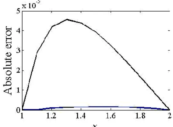
One can see from Table 1 that the absolute error in compact method is smaller than the absolute error obtained through finite difference scheme. A comparison of the absolute errors obtained through both of the above mentioned schemes is depicted in Fig. 1 showing that the results obtained by compact compact method are closer to the true solutions than that of the finite difference method. This means that the compact scheme gives more accurate results than the finite difference scheme.

3.2 Test Example 2

Consider the problem

, 2 1 ), sin(ln 5

3 2

2 _{    }

x x

x z z x z x

with the boundary conditions

z(1)=1,

z

(2)=2

The exact solution of this problem is

 

x2[C₁sin(ln x) C₂cos(lnx)]

z

) (ln ln

2 2

1_{x xcox x}

where C₁ and C₂ are given as C1= –0.004133291951, C2 = 1

The results obtained by using compact method and the finite difference method are tabulated below in Table 2. The table shows that the absolute error in compact method is smaller than the absolute error obtained through finite difference scheme. Figure 2 shows the comparison of the solutions obtained by the two schemes with that of the exact solution.

Fig. 1 Comparison of the absolute errors obtained through the two schemes. The upper black curve represents the absolute error using finite difference scheme and the lower blue curve shows the absolute error using compact scheme. Clearly, the absolute error obtained through compact scheme is closer to zero as compared with the finite difference scheme.

Fig. 2 Comparison of the absolute errors obtained through the two schemes. The upper black curve represents the absolute error using finite difference scheme and the lower blue curve (looks horizontal line) shows the absolute error using compact scheme. Clearly, the absolute error obtained through compact scheme is much closer to zero than that of the finite difference scheme.

Table 1 Comparison of the results obtained through the compact scheme and the finite difference scheme with that of the exact solution.

X Computed values by _{compact method finite difference method} Computed values by Exact values Absolute error in _{compact method} Absolute error in compact _method 1.0 1.000000000000000 1.000000000000000 1.000000000000000 0.000000000000000E-000 0.000000000000000E-000 1.1 1.092629320542001 1.092600520720135 1.092629298492154 2.204984728138015E-008 2.877073986828904E-005 1.2 1.187083959579468 1.187043128795073 1.187084840503766 8.809242986185239E-007 4.170367710476519E-005 1.3 1.283381173619071 1.283336870214396 1.283382364107264 1.190488193136829E-006 4.548491274070088E-005 1.4 1.381444549560547 1.381402046228608 1.381445951732330 1.402171783349004E-006 4.389561194684255E-005 1.5 1.481157904474377 1.481120262112219 1.481159417041742 1.512567365358208E-006 3.914415348749145E-005 1.6 1.582390912373861 1.582359895693457 1.582392460804419 1.548430557996028E-006 3.255347142738785E-005 1.7 1.685012497115571 1.684989018384561 1.685013961787879 1.464672307216475E-006 2.493091630695332E-005 1.8 1.788897387186686 1.788881746193746 1.788898534701186 1.147514499422186E-006 1.677518551668200E-005 1.9 1.893928779769380 1.893921099157133 1.893929509275649 7.295062691703436E-007 8.395971669461488E-006 2.0 2.000000000000000 2.000000000000000 2.000000000000000 0.000000000000000E-000 0.000000000000000E-000

Table 2 Comparison of results obtained through the compact scheme and the finite difference scheme with that of the exact solution.

x Computed values by _{compact method finite difference method} Computed values by Exact values Absolute error in compact _method Absolute error in compact _method 1.0 1.000000000000000 1.000000000000000 1.000000000000000 0.000000000000000E-000 0.000000000000000E-000 1.1 1.146630326188217 1.146917673363082 1.146631416625184 1.090436967610131E-006 2.862567378976166E-004 1.2 1.285956160227458 1.286455879241980 1.285957682261418 1.522033960865699E-006 4.981969805610831E-004 1.3 1.416242366015879 1.416884457613361 1.416244389090452 2.023074572310435E-006 6.400685229090985E-004 1.4 1.536163647969564 1.536882390484765 1.536166256830638 2.608861074504532E-006 7.161336541265939E-004 1.5 1.644733259061941 1.645466684938248 1.644736212251976 2.953190035182018E-006 7.304726862717992E-004 1.6 1.741244697570801 1.741934751120485 1.741247848563706 3.150992904821237E-006 6.869025567788345E-004 1.7 1.825225596606700 1.825817431936998 1.825228478874028 2.882267328363497E-006 5.889530629694661E-004 1.8 1.896398417154948 1.896840481563548 1.896400610158785 2.193003836747920E-006 4.398714047626484E-004 1.9 1.954648928821055 1.954892786170612 1.954650146329683 1.217508628137409E-006 2.426398409287600E-004 2.0 2.000000000000000 2.000000000000000 2.000000000000000 0.000000000000000E-000 0.000000000000000E-000

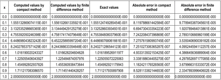
Table 3 Comparison of results obtained through the compact scheme and the finite difference scheme with that of the exact solution.

x Computed values by _{compact method} Computed values by finite _{difference method} Exact values Absolute error in compact _method Absolute error in finite _{difference method} 0.0 0.000000000000000E-000 0.000000000000000E-000 0.000000000000000E-000 0.000000000000000E-000 0.000000000000000E-000 0.1 1.555132869074115E-001 1.556102661335921E-001 1.555124749285454E-001 8.119788661442584E-007 9.778945387045601E-005 0.2 3.132535298665365E-001 3.134449429125279E-001 3.132528603934931E-001 6.694730433354223E-007 1.920789464013861E-004 0.3 4.755392050246398E-001 4.758174174079648E-001 4.755384808037960E-001 7.242208437396869E-007 2.789310666960199E-004 0.4 6.448698043823242E-001 6.452225885997204E-001 6.448690768061661E-001 7.275761580993745E-007 3.535040690039182E-004 0.5 8.240278537571429E-001 8.244366633354648E-001 8.240271286544123E-001 7.251027306365287E-007 4.095244594112257E-004 0.6 1.016190020243327 1.016628204604628 1.016189526911977 4.933313502153425E-007 4.386645636889064E-004 0.7 1.225055406043927 1.225484874057976 1.225055072225063 3.338188634405270E-007 4.297852697177085E-004 0.8 1.454992802937826 1.455360938473644 1.454992921179943 1.182421176526560E-007 3.679966315333072E-004 0.9 1.711217083086570 1.711451440428257 1.711217935897908 8.528113382144653E-007 2.334789399640602E-004 1.0 2.000000000000000E-000 2.000000000000000E-000 2.00000000000000E-000 0.000000000000000E-000 0.000000000000000E-000

3.3 Test Example 3

The linear second order boundary value problem ,

1 0 , 4

4   



 x x x

z

with the boundary conditions

, 2 ) 1 ( ,

0 ) 0

(  z 

z

has the exact solution

x e

e

z x x

e

e _{ }

 

 ( )

2 2 1

4 2

Table 3 shows that the absolute error in compact method is smaller than the absolute error obtained through the finite difference scheme. Figure 3 shows the comparison between the absolute errors of the two schemes.

4. Conclusions

In this work, the numerical solution of linear second order boundary value problems has been found using the compact method of order four. The specialty of the compact method is that it uses only three nodal points to get an accuracy of order four. The finite difference method was also employed to solve the same boundary value problems. The applicability and the validity of two schemes were examined by solving three test problems. It was found that the results obtained through compact method are closer to the actual results as compared to that of the finite difference approach.

5. References

[1] Kreiss, H.O. 1975, Methods for the approximate solution of time dependent problems. GARP Report No. 13.

[2] Hirsh, R.S. 1975, Higher order accurate difference solutions of fluid mechanics problems by a compact differencing technique, Journal of Computational Physics, Vol. 19 (1). pp 90–109.

[3] Adam, Y. 1977, Highly accurate compact implicit methods and boundary conditions, Journal of Computational Physics, Vol. 24 (1). pp 10–22.

[4] Leventhal, S.H., Ciment, M. 1978, A note on the operator compact implicit method for the wave equation. Mathematics of Computation. Vol. 32 (1). pp 143-147.

[5] Dennis, S.C.R., Hudson, J.D. 1989, Compact

4

h finite-difference approximations to operators of Navier-Stokes type, Journal of Computational Physics. Vol. 85 (2). pp 390– 416.

[6] Ahmad, M.O.; An Exploration of Compact Finite Difference-methods for Numerical Solution of PDE, Ph.D. Thesis, University of Western, Ontario, Canada, (1997).

[7] Burden, R.L., Faires, J.D. 2010, Numerical Analysis. International Thomson Publishing Inc, New York, USA.