Research Article Effects of the Offset Term in Experimental Simulation on Afterglow Decay Curve

(1)

Research Article

Effects of the Offset Term in Experimental Simulation on

Afterglow Decay Curve

Chi-Yang Tsai,

1,2

Jeng-Wen Lin,

3

Yih-Ping Huang,

3

and Yung-Chieh Huang

4

1_{Graduate Institute of Dentistry, College of Oral Medicine, Taipei Medical University, Taipei 110, Taiwan}

2_{Department of Dentistry, Taipei Medical University Hospital, Taipei 110, Taiwan}

3_{Department of Civil Engineering, Feng Chia University, Taichung 407, Taiwan}

4_{Department of Pediatrics, Taichung Veterans General Hospital, Taichung 407, Taiwan}

Correspondence should be addressed to Jeng-Wen Lin; [email protected] Received 17 March 2014; Accepted 29 May 2014; Published 26 June 2014 Academic Editor: Faik Oktar

Copyright © 2014 Chi-Yang Tsai et al. This is an open access article distributed under the Creative Commons Attribution License, which permits unrestricted use, distribution, and reproduction in any medium, provided the original work is properly cited. This study examines the effect of the offset term in a multiple single exponential equation that fits into experimental afterglow decay curve data for material applications. For afterglow materials applied and attached to structures, the inclusion of this offset term may reduce the values of the calculated decay times,𝜏_𝑖, and enlarge the time invariant constants,𝐴_𝑖, in the associated equation compared to theoretically perfect test conditions. Using a set of experimental data obtained from a lab under dim light, adjustments can be made to calculate the required parameters for an equation without the offset term. This study uses mathematical simulations and lab tests to support our thesis and crosslink test results generated from different ambient light conditions. This paper defines the offset ratio as the ratio of the offset value,𝐼₀, versus the initial light intensity in an equation. This ratio can be used to evaluate possible effects on the calculated parameters of an equation in an associated numerical simulation. The most reliable parameters will have consistent results from the use of multiple single exponential equations, with and without the offset term, in simulations to obtain them in an equation to model a set of data.

1. Introduction

Many researchers commonly use empirical multiple single exponential equations to fit experimental curve data [1]. If a lab is unable to completely block ambient light or luminous intensity is not measured for a sufficient time period, residual light will appear in the test data, indicated by the offset term (𝐼₀) as follows:

𝐼 = 𝐼₀+∑𝑛

𝑖=1

𝐴_𝑖exp(−𝑡

𝜏_𝑖) , (1)

where𝐼 is the light intensity at any time,𝑡, after switching off the excitation illumination, 𝐼₀ is the offset term that represents residual light, and𝐴_𝑖is a time-invariant constant. The term 𝜏_𝑖 is a decay constant (or decay time) for the exponential components. A choice can be made from among

𝑛 = 1as single, 𝑛 = 2 as double, and 𝑛 = 3as triple exponential equations.

𝐼₀was identified as background by Pedroza-Montero et al. and as background intensity by Chen et al. [2,3]. In order to solve (1), the 𝐼₀ term can be computed independently and subtracted from the 𝐼 equation [4]. By quoting the physical properties of experimental data, Huang et al. showed methods to examine the definition for associated parameters in an equation and solve them [5]. Using log coordinates, Sharma et al. indicated that a decay curve, such as (1), can be treated as the minimum number of straight lines with slow, medium, and fast components, and each line represents a different light intensity stage [6]. In other words,𝐼₀ should not exist in good experimental data, and its influence on modeling must be investigated.

Theoretically,𝐼₀should be zero in (1), and it is appropriate to use a zero value if the obscure light in the lab room is eliminated:

𝐼 =∑𝑛

𝑖=1

𝐴_𝑖exp(−𝑡

𝜏_𝑖) . (2)

Volume 2014, Article ID 497270, 9 pages http://dx.doi.org/10.1155/2014/497270

(2)

(2) Small𝐼₀ PET 9.200 0.0957 0.010

(3) Medium𝐼₀ PET 9.200 0.1601 0.017

(4) No𝐼₀ UV 6.400 0.000 0.000

(5) Small𝐼₀ UV 6.400 0.0775 0.012

(6) Medium𝐼₀ UV 6.400 0.1774 0.028

The problem is that many researchers still use (1) for their studies [7–11]. This raises four questions.

(1) Does the ambient light in a test affect the afterglow data locally or globally in a numerical simulation? (2) Can we adjust the experimental data received from

a dim light environment to simulate that from a completely dark environment?

(3) How does the difference in the calculated parameters used in (1) compare with (2)?

(4) When can we stop an afterglow experimental test, even under perfect conditions?

This study focuses on answering the above questions using mathematical simulations and lab tests to support our results, that is, to find the effect of experimental data obtained from a dim light lab on the calculated parameters of an equation. Some dim light that exists in labs may be at an acceptable level, and the measured data can be adjusted for this using the conditions proposed in this paper. On the other hand, this may cause interpolation problems for experimental data obtained from a test that was not measured until the light intensity,𝐼, was approximately zero.

2. Offset Ratio

Several lab tests were executed to study the effect of ambient light on the afterglow decay curve simulation.Table 1assigns the different conditions to the tests. Two kinds of patches were involved, PET resin and UV. The initial light intensity is expressed in (3), and the offset ratio (𝑅) in (4) is defined as the ratio of the offset value (𝐼₀) versus the initial light intensity

(𝐼initial):

𝐼initial= 𝐼0+

𝑛

∑

𝑖=1

𝐴_𝑖, (3)

𝑅 = _𝐼𝐼0

initial

, (4)

where𝑅is the offset ratio in this paper,𝐼initialis the initial light

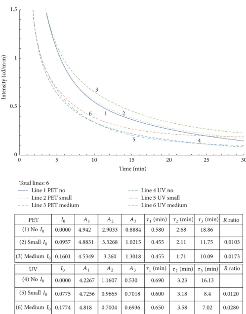
intensity in a test, and𝐼₀is the offset value of an equation. It is obvious that with a larger offset ratio value (𝑅), the processed curve (with 𝐼₀) will greatly diverge from a perfect one (without𝐼₀).Figure 1depicts the decay curves and calculated parameters for all the cases described inTable 1. In

this figure, there are three curves for PET (curves 1–3) and UV (curves 4–6) resins that are identical at the beginning. However, they gradually diverge at some point in time. Evidence shows that the ambient light only effects curves locally, but the diverge point is far away from the offset value,

𝐼₀. The calculated parameters for these cases are tabulated on the lower side of the figure. They were calculated using triple exponential equations. Examination of the first three curves reveals that the largest is𝜏₃in curve 1 (no𝐴₀) calculated using (2). Curves 2-3 use (1) to compute the associated parameters. The results indicate that with an increase in the ambient light intensity, 𝜏₃ decreases with the increase of 𝐴₃. The same behavior can be observed in curves 4–6. In that figure, curves 1 and 4 represent the perfect environmental testing, and the calculated parameters in the equation are regarded as correct. In other words, the cases performed with some ambient light will lead to an underestimation of the calculated decay times and an overestimation of the time-invariant constants.𝜏₃ is usually taken to correlate to some phosphor behaviors [7–11].

3. The Quality of the Experimental Data

The quality of the experimental data is of vital importance for generating representative equations in curve simulations. In addition to accuracy in reading and machinery, there are several crucial processes that have to be dealt with, such as environmental and temperature controls, the time interval for data reading, and the duration of the test. Automatic reading by computer is required for such tests because the data can be measured within seconds. This also minimizes human error in reading the data. Another crucial issue is how much time is required for a good measurement. The next paragraph will focus on this subject.

Ideally, it is better to prolong a test as long as possible until the calibration limit is reached; however, this may mean that several hours are required for a single test run. The cost of an insufficient data duration for a numerical process is that variations in the equation interpolation will be part of the outcome. An easy way to identify this problem is to apply the two equations separately, with and without the offset term, such as with (1) and (2). Then, check to see if the corresponding parameters in the two equations have similar values. If they are in agreement with each other, then the data are appropriate for use. This may also mean the calculated parameters are acceptable.

(3)

0 0.5 1 1.5

0 5 10 15 20 25 30

In

te

n

si

ty (cd/m

·

m)

Time (min) Total lines: 6

Line 1 PET no Line 2 PET small Line 3 PET medium

Line 4 UV no Line 5 UV small Line 6 UV medium

PET R ratio

R ratio

0.0000 4.942 2.9033 0.8884 0.580 2.68 18.86

0.0957 4.8831 3.3268 1.0215 0.455 2.11 11.75 0.0103

0.1601 4.5349 3.260 1.3018 0.455 1.71 10.09 0.0173

UV

0.0000 4.2267 1.1607 0.530 0.690 3.23 16.13

0.0775 4.7256 0.9665 0.7018 0.600 3.18 8.4 0.0120

0.1774 4.818 0.7004 0.6936 0.650 3.58 7.02 0.0280

5 4

6 3

1 2

I0 A1 A2 A3 𝜏1(min) 𝜏2(min) 𝜏3(min)

(4) No _I0

(5) Small I₀

(6) Medium _I0

(3) Medium I₀

(2) Small I₀

(1) NoI₀

Figure 1: Decay curves used in this study as defined inTable 1.

Table 2: Simulated by using equations with the𝐼₀term.

Source 𝐼₀ 𝐴₁ 𝐴₂ 𝐴₃ 𝜏₁ 𝜏₂ 𝜏₃ 𝐼₀/𝐼_initial

Original 0.0 4.90 2.90 0.87 0.60 2.70 16.90

120 min 0.00223 4.9078 2.8833 0.878 0.60 2.70 16.55 0.026%

60 min 0.01327 4.7920 2.9271 0.942 0.59 2.54 15.14 0.153%

48 min 0.02047 4.7979 2.9127 0.945 0.59 2.54 14.74 0.236%

40 min 0.14750 3.2756 3.2200 2.049 0.50 1.24 6.17 1.697%

30 min 0.18213 3.5000 3.0774 1.942 0.50 1.34 6.06 2.093%

Using some predefined parameters for a specific curve description in this study, we generated a set of data points that represent the curve before the separate application of (1) and (2) to compute the associated parameters in the equations. The data points are tabulated in Tables 2 and 3. If sufficient data are applied in the numerical interpola-tion, then, theoretically, regardless of the type of equation involved, a consistent result should be achieved. That is to say,

the calculated parameters should be similar to the predefined parameters.

This study used data points that extend up to 120 min in the decay process and collected the calculated parameters in Tables 2 and 3. In both tables, the second row marked as “original” represents the predefined parameters in an afterglow equation and the third row marked as “120 min” shows the parameters calculated by including data points

(4)

60 min 0.00 4.8727 2.9236 0.8795 0.595 2.67 16.74

30 min 0.00 4.8725 2.9239 0.8793 0.595 2.67 16.74

14 min 0.00 4.8875 2.8750 0.9250 0.600 2.66 16.08

9 min 0.00 4.8945 2.8388 0.9360 0.600 2.65 15.15

6 min 0.00 4.6317 2.2197 1.8210 0.585 1.91 7.59

0 0.5 1 1.5

0 5 10 15 20 25 30

Time (min) 2

3 2

0.0000 4.2267 1.1607 0.530 0.690 3.23 16.13

0.0775 4.7256 0.9665 0.7018 0.60 3.18 8.4

0.0000 4.6524 1.1976 0.6345 0.59 2.98 13.48

UV

0.0000 4.942 2.9033 0.8684 0.580 2.66 16.86

0.0957 4.8831 3.3268 1.0215 0.455 2.11 11.75

0.0000 4.927 2.87 0.891 0.580 2.61 17.31

1

6 4 5

5

PET

(6) Modify (3) Modify

I0 A1 A2 A3 𝜏1(min)𝜏2(min)𝜏3(min)

Line 1 no Line 2 small Line 3 modify

Line 4 no Line 5 smal Line 6 modify Total lines: 6

(4) No I₀

(5) Small I0

(2) Small _I0

(1) No I₀

In

te

n

si

ty (cd/m

·

m)

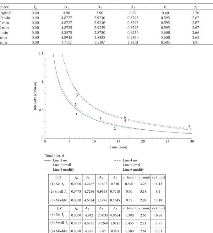
Figure 2: Modified curves with small𝑅values fromFigure 1. within a 120 min duration in the numerical process, and the

same is true for “60 min” and other cases.

The data inTable 2are calculated using an equation with the𝐼₀term. It seems that 120 min is fine for the comparison with an opponent as without 𝐼₀ case (Table 3) but with a slightly smaller𝜏₃.Table 2reveals that fewer data points in the interpolation can result in larger𝐼₀values and small𝜏₃values. The last column is the offset ratio,𝑅, and the𝑅value is a direct response to the divergence of the calculated parameters. The smaller 𝑅 value gives better results for interpolation. This study recommends that this value be kept below 1.0%, as seen

in the example used here.Table 3indicates that the calculated parameters are acceptable with inclusion of the data for more than 30 min. It is obvious that diverse results can be found in 9 min or less. Therefore, it is important to use the equation model without the𝐼₀term for interpolation of an afterglow decay curve test.

4. Data Computational Adjustment

In Figure 1, curves 1 and 4 are used and the other curves resulted from imperfect testing conditions such as dim light.

(5)

0 0.5 1 1.5

0 5 10 15 20 25 30

In

te

n

si

ty (cd/m

·

m)

Time (min)

0.0000 4.942 2.9033 0.8684 0.580 2.66 16.86

0.1601 4.5349 3.2600 1.3018 0.455 1.71 10.09

0.0000 4.7328 3.1706 1.2886 0.48 1.91 14.01

UV

0.0000 4.2267 1.1607 0.530 0.690 3.23 16.13

0.1774 4.8180 0.7004 0.6936 0.650 3.56 7.020

0.0000 4.7858 0.8785 0.6824 0.660 3.47 14.47

2 4

6 5

1

3

PET _I0 A1 A2 A3 𝜏₁(min) _𝜏2(min) 𝜏₃(min)

I0 A1 A2 A3 𝜏1(min) 𝜏2(min) 𝜏3(min)

Total lines: 6

(6) Modify (3) Modify

(4) No I₀

(1) No I₀

(2) Medium I₀

(5) Medium I₀

Line 1 no

Line 2 medium Line 5 medium

Line 3 modify

Line 4 no Line 6 modify

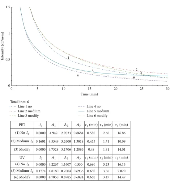
Figure 3: Modified curves with medium𝑅values fromFigure 1.

How can we transform curves 2-3 into curve 1 or 5 and curve 6 into curve 4?

To revise the 𝜏_𝑖 value calculated from (1), the lab data were adjusted by abandoning the last several terms that were smaller than the𝐼₀ term. Then, the data were reprocessed with (2). The results are plotted in Figures2and3for small and medium𝑅values, respectively. The simulation had great results for the associated𝜏₃ values. With larger𝑅values, it is less likely that a good approximation can be achieved by merely trimming off the original data for the modification process as proposed. This topic deserves further study in the future.

5. Results and Discussion

In this section, the proposed scheme discussed in the previ-ous section is applied to the data reported in five different articles [7–11] for demonstration. We purposely chose cases processed with the offset term in a numerical approximation (1), and we recalculated for the parameters in (2) by removing the last several terms in the data. In other words, using

the given parameters of an equation in previous articles, the experimental data along a decay curve can be recreated, and the last portion of the curve that is close or below the offset value is eliminated. The remaining data are used to generate a new curve from (2).Figure 4illustrates the first example. The calculated parameters are tabulated in the upper right hand side of the figure and include the original data as well as the data created for this study. The𝑅value is 5.44%. This value is thought to be proportional to the difference between the two curves and their slow-decay times (𝜏₃). The mismatch of 4.623 versus 23.19 for the two slow-decay times,𝜏₃, in this example indicates that either the𝑅value used is too large or (1) cannot be used to model this case.

In examples 2–4 from Figures5,6, and7, the 𝑅values are within 0.7%–6.8%. The regenerated curves and calculated parameters,𝐴_𝑖and𝜏_𝑖, are close to the original documented source. The results show that the calculated slow-decay times (𝜏₂or𝜏₃) are approximately 2 times the original values.

Example 5 shows an extreme situation with𝑅values as high as 10.44%.Figure 8 shows that the modified curve is close to the original one. However, the difference between the two slow-decay time values (𝜏₂) in the table is 6 times greater.

(6)

0 0.5 1

0 5 10 15 20 25 30

In

te

n

si

ty (cd/m

·

m)

Line 1 Sun and Zhao Line 2 this study Authors

(1) Sun and Zhao 0.22 2.879 0.689 0.252 0.128 0.7227 4.6237 0.0544

(2) This study 0.00 2.879 0.781 0.383 0.125 0.830 23.19

1 2

R ratio

I0 A1 A2 A3 _𝜏1(min)_𝜏2(min)𝜏3(min)

Figure 4: Example 1 with modified data from [7].

0 0.5 1 1.5

0 5 10 15 20 25 30

In

te

n

si

ty (cd/m

·

m)

Line 1 Han et al. Line 2 this study

2

Authors

(1) Han et al. 0.06775 8.4120 0.5741 0.8029 8.623 0.00748

(2) This study 0.00000 8.4704 0.5550 0.8200 13.420

1

R ratio

I0 A1 A2 𝜏1(min) 𝜏2(min)

(7)

Authors

(1) Chang et. al. 0.315 2.027 1.8348 0.4212 0.0566 0.390 1.82 0.0685

(2) This study 0.00 2.6307 1.4475 0.2561 0.085 0.430 3.74

0 0.5 1 1.5

0 5 10 15 20 25 30

In

te

n

si

ty (cd/m

·

m)

Time (min) Total lines-2

Line 1 Chang et. al. Line 2 this study

1

2

R ratio

I0 A1 A2 A3 _𝜏1(min) 𝜏2(min)_𝜏3(min)

0 0.5 1 1.5

0 5 10 15 20 25 30

In

te

n

si

ty (cd/m

·

m)

Line 1 Sharma et al. Line 2 this study

2

Authors

(1) Sharma et al. 0.03616 2.6402 1.1992 0.13592 0.94309 0.00933

(2) This study 0.00000 2.8204 1.05167 0.150 1.180

1

R ratio

(8)

Authors

(1) Lei et al. 0.4787 3.5750 0.5318 0.5735 4.7678 0.1044

(2) This study 0.0000 3.7489 0.8083 0.6260 29.510

0 0.5

0 5 10 15 20 25 30

In

te

n

si

ty (cd/m

Time (min) Total line: 2

Line 1 Lei et al. Line 2 this study

2 1

R ratio

This shows that the experimental environment for afterglow luminescence measurements should be taken seriously.

6. Conclusions

It is common to retain dim light in afterglow experimental tests for different reasons, including easy operation, operator friendliness or ease of use, and physical chemistry appli-cations of afterglow decay curve data. However, if such experimental data is directly used for numerical simulations, the consequence of having an offset term in the equation may cause confusion. The offset ratio is used to evaluate the possible effect of the offset term. This study points out that increasing the offset ratio may decrease the calculated slow-decay time (𝜏₂or𝜏₃) from the use of (1) in interpolation, that is, mainly affecting the slow-decay time component in that equation. An adjustment scheme to modify the experimental data was proposed, and it was valid for compensating for the offset term effect in the equations. That is, a perfectly dark lab room may not be required to run the associated afterglow measurements. From the examples in this study, we recommend that the offset ratio should be less than 1.0% for such a test. The two equations, with and without offset terms, were used for a numerical process and then the generated parameters from these two equations were compared to examine the quality of the obtained experimental data.

Conflict of Interests

The authors declare that there is no conflict of interests regarding the publication of this paper.

Acknowledgments

The work described in this paper consists of research projects under the auspices of the National Science Council, Taiwan,

under Contract nos. NSC 96-2221-E-035-038, NSC 101-2221-E-035-023, and NSC 102-2221-E-035-049, and the support is greatly appreciated.

References

[1] K. Holmstr¨om and J. Petersson, “A review of the parameter estimation problem of fitting positive exponential sums to empirical data,”Applied Mathematics and Computation, vol. 126, no. 1, pp. 31–61, 2002.

[2] M. Pedroza-Montero, B. Castañeda, M. I. Gil-Tolano, O. Arellano-Tánori, R. Meléndrez, and M. Barboza-Flores, “Dose effects on the long persistent luminescence properties of beta irradiated SrAl₂O₄:Eu2+, Dy3+ phosphor,”Radiation Measure-ments, vol. 45, no. 3–6, pp. 311–313, 2010.

[3] Y. Chen, X. Cheng, M. Liu, Z. Qi, and C. Shi, “Comparison study of the luminescent properties of the white-light long afterglow phosphors: Ca_𝑥MgSi₂O_5+𝑥:Dy3+(𝑥 = 1, 2, 3),”Journal of Luminescence, vol. 129, no. 5, pp. 531–535, 2009.

[4] J. R. Knisley and L. L. Glenn, “A linear method for the curve fitting of multiexponentials,”Journal of Neuroscience Methods, vol. 67, no. 2, pp. 177–183, 1996.

[5] Y. Huang, C. Tsai, and Y. Huang, “Mathematical modeling of afterglow decay curves,” inDesign and Computation of Modern

Engineering Materials, A. ¨Ochsner and H. Altenbach, Eds., vol.

54 ofAdvanced Structured Materials, Springer International Publishing AG, New York, NY, USA, 2014.

[6] S. K. Sharma, S. S. Pitale, M. M. Malik, R. N. Dubey, and M. S. Qureshi, “Luminescence studies on the blue-green emitting Sr₄Al₁₄O₂₅:Ce3+phosphor synthesized through solution com-bustion route,”Journal of Luminescence, vol. 129, no. 2, pp. 140– 147, 2009.

[7] F. Sun and J. Zhao, “Blue-green BaAl₂O₄:Eu2+,Dy3+ phos-phors synthesized via combustion synthesis method assisted by microwave irradiation,”Journal of Rare Earths, vol. 29, no. 4, pp. 326–329, 2011.

(9)

[8] S. Han, K. C. Singh, T. Cho et al., “Preparation and characteriza-tion of long persistence strontium aluminate phosphor,”Journal of Luminescence, vol. 128, no. 3, pp. 301–305, 2008.

[9] C. Chang, W. Li, X. Huang et al., “Photoluminescence and afterglow behavior of Eu2+, Dy3+and Eu3+, Dy3+in Sr₃Al₂O₆ matrix,”Journal of Luminescence, vol. 130, no. 3, pp. 347–350, 2010.

[10] B. Lei, S. Man, Y. Liu, and S. Yue, “Luminescence properties of Sm3+-doped Sr₃Sn₂O₇ phosphor,”Materials Chemistry and Physics, vol. 124, no. 2-3, pp. 912–915, 2010.

[11] S. K. Sharma, S. S. Pitale, M. M. Malik et al., “Spectral and defect analysis of Cu-doped combustion synthesized new SrAl₄O₇ phosphor,”Journal of Luminescence, vol. 130, no. 2, pp. 240–248, 2010.

(10)

Submit your manuscripts at

http://www.hindawi.com

Hindawi Publishing Corporation

http://www.hindawi.com Volume 2014

Inorganic Chemistry International Journal of

Carbohydrate

Chemistry

International Journal of

http://www.hindawi.com Volume 2014 Journal of

Chemistry

Hindawi Publishing Corporation http://www.hindawi.com

Analytical Methods in Chemistry

Journal of

Volume 2014

Bioinorganic Chemistry and Applications Hindawi Publishing Corporation

Spectroscopy

The Scientific

World Journal

Chromatography Research International Hindawi Publishing Corporation

Applied ChemistryJournal of Hindawi Publishing Corporation

Theoretical Chemistry

Journal of Hindawi Publishing Corporation

Journal of

Spectroscopy

Journal of

http://www.hindawi.com Volume 2014 Quantum Chemistry

Research Article Effects of the Offset Term in Experimental Simulation on Afterglow Decay Curve