8 Magnetism
8.1
Introduction
The topic of this part of the lecture deals are the magnetic properties of materials. Most materials are generally considered to be “non-magnetic”, which is a loose way of saying that they become magnetized only in the presence of an applied magnetic field (dia- and paramagnetism). We will see that in most cases these effects are very weak, and the magnetization is lost, as soon as the external field is removed. Much more interesting (also from a technological point of view) are those materials, which not only have a large magnetization, but also retain it even after the removal of the external field. Such materials are called permanent magnets (ferromagnetism). The property that like (unlike) poles of permanent magnets repel (attract) each other was already known to the Ancient Greeks and Chinese over 2000 years ago. They used this knowledge for instance in compasses. Since then, the importance of magnets has risen steadily. Now they play an important role in many modern technologies:
• recording media (e.g. hard disks): data is recorded on a thin magnetic coating. The
revolution in information technology owes as much to magnetic storage as to infor-mation processing with computer chips (i.e. the ubiquitous silicon chip).
• credit, debit, and ATM cards: all of these cards have a magnetic strip on one side. • TVs and computer monitors: contain a cathode ray tube that employs an
electro-magnet to guide electrons to the screen. Plasma screens and LCDs use different technologies.
• speakers and microphones: most speakers employ a permanent magnet and a
current-carrying coil to convert electric energy (the signal) into mechanical energy (move-ment that creates the sound).
• Electric motors and generators: some electric motors rely upon a combination of
an electromagnet and a permanent magnet, and, much like loudspeakers, they con-vert electric energy into mechanical energy. A generator is the reverse: it concon-verts mechanical energy into electric energy by moving a conductor through a magnetic field.
• Medicine: Hospitals use magnetic resonance imaging to spot problems in a patient’s
organs without invasive surgery.
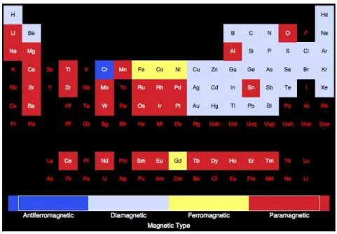
Figure 8.1: Magnetic type of the elements in the periodic table. For elements without a color designation magnetism is even smaller or not explored.
Figure 8.1 illustrates the type of magnetism in the elementary materials of the periodic table. Only Fe, Ni, Co and Gd exhibit ferromagnetism. Most magnetic materials are there-fore alloys or oxides of these elements or contain them in another form. There is, however, recent and increased research into new magnetic materials such as plastic magnets (or-ganic polymers), molecular magnets (often still based on transition metals) or molecule based magnets (in which magnetism arises from strongly localized s and p electrons). Electrodynamics gives us a first impression of magnetism. Magnetic fields act on moving electric charges or, in other words, currents. Very roughly one may understand the be-havior of materials in magnetic fields as arising from the presence of “moving charges”. (Bound) core and/or (quasi-free) valence electrons possess a spin, which in a simplified classical picture can be viewed as a rotating charge, i.e. a current. Bound electrons have an additional orbital momentum, which adds another source of current (again in a simplistic classical picture). These “microscopic currents” react in two different ways to an applied magnetic field: First, according to Lenz’ law a current is induced that creates a mag-netic field opposing the external magmag-netic field (diamagnetism). Second, the “individual magnets” represented by the electron currents align with the external field and enhance it (paramagnetism). If these effects happen for each “individual magnet” independently, they remain small. The corresponding magnetic properties of the material may then be understood from the individual behavior of the constituents, i.e. atoms/ions (insulators, semiconductors) or atoms/ions and free electrons (conductors), cf. section 8.3. The much stronger ferromagnetism, on the other hand, arises from a collective behavior of the “in-dividual magnets” in the material. In section 8.4 we will first discuss the source for such an interaction, before we move on to simple models treating either a possible coupling of localized moments or itinerant ferromagnetism.
8.2
Macroscopic Electrodynamics
Before we plunge into the microscopic sources of magnetism in solids, let us first recap a few definitions from macroscopic electrodynamics. In vacuum we have E and B as the electric field (unit: V/m) and the magnetic flux density (unit: Tesla = Vs/m2), respectively.
Note that both are vector quantities, and in principle they are also functions of space and time. Since we will only deal with constant, uniform fields in this lecture, this dependence will be dropped throughout. Inside macroscopic media, both fields can be affected by the charges and currents present in the material, yielding the two new net fields, D (electric displacement, unit: As/m2) and H (magnetic field, unit: A/m). For the formulation of
macroscopic electrodynamics (the Maxwell equations in particular) we therefore need so-called constitutive relationsbetween the external (applied) and internal (effective) fields:
D =D(E,B), H=H(E,B). (8.1)
In general, this functional dependence can be written in form of a multipole expansion. In most materials, however, already the first (dipole) contribution is sufficient. These dipole terms are called P(el. polarization) and M (magnetization), and we can write
H = (1/µo)B−M+. . . (8.2)
D = ǫoE+P+. . . , (8.3)
where ǫo = 8.85·10−12As/Vm and µo = 4π·10−7Vs/Am are the dielectric constant and
permeability of vacuum, respectively. P and M depend on the applied field, which we can formally write as a Taylor expansion in E and B. If the applied fields are not too strong, one can truncate this series after the first term (linear response), i.e. the induced polarization/magnetization is then simply proportional to the applied field. We will see below that external magnetic fields we can generate at present in the laboratory are indeed weak compared to microscopic magnetic fields, i.e. the assumption of a magnetic linear response is often well justified. As a side note, current high-intensity lasers may, however, bring us easily out of the linear response regime for the electric polarization. Corresponding phenomena are treated in the field of non-linear optics.
For the magnetization it is actually more convenient to expand in the internal field H instead of inB. In the linear response regime, we thus obtain for the induced magnetization and the electric polarization
M = (1/µo)χmag H (8.4)
P = ǫo χE, (8.5)
whereχel/mag is the dimensionless electric/magnetic susceptibility tensor. In simple
mate-rials (on which we will focus in this lecture), the linear response is often isotropic in space and parallel to the applied field. The susceptibility tensors then reduce to scalar form and we can simplify to
M = (1/µo)χmag H (8.6)
P = ǫoχel E. (8.7)
These equations are in fact often directly written as defining equations for the dimension-less susceptibilityconstantsin solid state textbooks. It is important to remember, however,
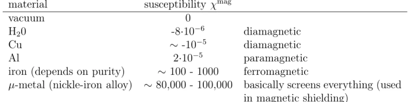
material susceptibility χmag
vacuum 0
H20 -8·10−6 diamagnetic
Cu ∼ -10−5 diamagnetic
Al 2·10−5 paramagnetic
iron (depends on purity) ∼ 100 - 1000 ferromagnetic
µ-metal (nickle-iron alloy) ∼80,000 - 100,000 basically screens everything (used in magnetic shielding)
Table 8.1: Magnetic susceptibility of some materials.
that we made the dipole approximation and restricted ourselves to isotropic media. For this case, the constitutive relations between external and internal field reduce to
H = 1
µoµr
B (8.8)
D = ǫoǫr E, (8.9)
where ǫr = 1 + χel is the relative dielectric constant, and µr = 1−χmag the relative
permeability of the medium. Forχmag <0, we haveµ < 1and|H|<|1
µ0B|. The response
of the medium reduces (or in other wordsscreens) the external field. Such a system is called diamagnetic. For the opposite case (χmag >0) we have µ > 1 and therefore |H|>|1
µ0B|.
The external field is enhanced by the material, and we talk about paramagnetism.
To connect to microscopic theories we consider the energy. The process of screening or enhancing the external field will require work, i.e. the energy of the system is changed (magnetic energy). Assume therefore that we have a material of volumeV, which we bring into a magnetic field B (which for simplicity we take to be along one dimension only). From electrodynamics we know that the energy of this magnetic field is
Emag = (1/2BH)V ⇒ 1/V dEmag = 1/2BdH+ 1/2HdB. (8.10)
From eq. (8.9) we find dB=µoµrdH and therefore HdB =BdH, which leads to
1/V dEmag =BdH = (µoH+µoM)dH =BodH+µoMdH. (8.11)
In the first term, we have realized that µoH = Bo is just the field in the vacuum, i.e.
without the material. This term therefore gives the field induced energy change, if no material was present. Only the second term is material dependent and describes the energy change of the material in reaction to the applied field. The energy change of the material itself is therefore
dEmaterialmag =−µoMV dH. (8.12)
Recalling that the energy of a dipole with magnetic moment m in a magnetic field is E = −mB, we see that the approximations leading to eq. (8.9) mean nothing else but assuming that the homogeneous solid is build up of a constant density of “molecular dipoles”, i.e. the magnetizationM is the (average) dipole moment density.
Rearranging eq. (8.12), we arrive finally at an expression that is a special case of a fre-quently employed alternative definition of the magnetization
M(H) = − 1 µoV ∂E(H) ∂H S,V , (8.13)
and in turn of the susceptibility χmag(H) = ∂M(H) ∂H S,V = − 1 µoV ∂2E(H) ∂H2 S,V . (8.14)
At finite temperatures, it is straightforward to generalize these definitions to M(H, T) =− 1 µoV ∂F(H, T) ∂H S,V χmag(H, T) =− 1 µoV ∂2F(H, T) ∂H2 S,V . (8.15) While the derivation via macroscopic electrodynamics is most illustrative, we will see that these last two equations will be much more useful for the actual quantum-mechanical computation of the magnetization and susceptibility of real systems. All we have to do, is to derive an expression for the energy of the system as a function of the applied external field. The first and second derivatives with respect to the field then yield M and χmag,
respectively.
8.3
Magnetism of atoms and free electrons
We had already discussed that magnetism arises from the “microscopic currents” con-nected to the orbital and spin moments of electrons. Each electron therefore represents a “microscopic magnet”, but how do they couple in materials, with a large number of electrons? Since any material is composed of atoms it is reasonable to first reduce the problem to that of the electronic coupling inside an atom, before attempting to describe the coupling of “atomic magnets”. Since both orbital and spin momentum of all bound electrons of an atom will contribute to its magnetic behavior, it will be useful to first re-call how the total electronic angular momentum of an atom is determined (section 8.3.1), before we turn to the effect of a magnetic field on the atomic Hamiltonian (section 8.3.2). In metals, we have the additional presence of free conduction electrons, the magnetism of which will be addressed in section 8.3.3. Finally, we will discuss in section 8.3.4, which aspects of magnetism we can already understand just on the basis of these results on atomic magnetism, i.e. in the limit of vanishing coupling between the “atomic magnets”.
8.3.1
Total angular momentum of atoms
In the atomic shell model, the possible quantum states of electrons are labeled as nlml,
where n is the principle quantum number, l the orbital quantum number, and ml the orbital magnetic quantum number. For any givenn, defining a so-called “shell”, the orbital
quantum numberlcan take only integer values between 0 and(n−1). Forl = 0,1,2,3. . ., we generally use the letters s,p, d,f and so on. Within such an nl “subshell”, the orbital magnetic number ml may have the (2l+ 1) integer values between −l and +l. The last
quantum number, the spin magnetic quantum number ms, takes the values −1/2 and
+1/2. For the example of the first two shells this leads to two 1s, two 2s, and six 2p states.
When an atom has more than one electron, the Pauli exclusion principle dictates that
each quantum state specified by the set of four quantum numbers nlmlms can only be
occupied by one electron. In all but the heaviest ions, spin-orbit coupling1 is negligible. In 1
this case, the Hamiltonian does not depend on spin or the orbital moment and therefore commutes with these quantum numbers (Russel-Saunders coupling). The total orbital and spin angular momentum for a given subshell are then good quantum numbers and are given by
L=Xml and S =
X
ms. (8.16)
If a subshell is completely filled, it is easy to verify that L=S=0. The total electronic angular momentum of an atomJ =L+S, is therefore determined by the partially filled subshells. The occupation of quantum states in a partially filled shell is given by Hund’s rules:
1. The states are occupied so that as many electrons as possible (within the limitations of the Pauli exclusion principle) have their spins aligned parallel to one another, i.e., so that the value of S is as large as possible.
2. When determined how the spins are assigned, then the electrons occupy states such that the value ofL is a maximum.
3. The total angular momentum J is obtained by combiningL and S as follows:
• if the subshell is less than half filled (i.e., if the number of electrons is<2l+ 1), then J =L−S;
• if the subshell is more than half filled (i.e., if the number of electrons is>2l+1), then J =L+S;
• if the subshell is exactly half filled (i.e., if the number of electrons is = 2l+ 1), then L= 0, J =S.
The first two Hund’s rules are determined purely from electrostatic energy considera-tions (e.g. electrons with equal spins are farther away from each other on account of the exchange-hole). Only the third rule follows from spin-orbit coupling. Each quantum state in this partially filled subshell is called amultiplet. The term comes from the spectroscopy
community and refers to multiple lines (peaks) that have the same origin (in this case the same subshell nl). Without any interaction (e.g. electron-electron, spin-orbit, etc.) all quantum states in this subshell would be energetically degenerate and the spectrum would show only one peak at this energy. The interaction lifts the degeneracy and in an ensemble of atoms different atoms might be in different quantum states. The single peak then splits into multiple peaks in the spectrum. The notation for theground-state multiplet, obtained
by Hund’s rules is not simply denotedLSJ as one would have expected. Instead, for histor-ical reasons, the notation(2S+1)L
J is used. To make matters worse, the angular momentum
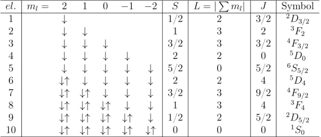
symbols are used for the total angular momentum (L= 0,1,2,3, . . .=S, P, D, F, . . .). The rules are in fact easier to apply than their description might suggest at first glance. Table 8.2 lists the filling and notation for the example of a d-shell.
8.3.2
General derivation of atomic susceptibilities
Having determined the total angular momentum of an atom, we now turn to the effect of a uniform magnetic field H (taken along the z-axis) on the electronic Hamiltonian of an atom He=Te+Ve−ion+Ve−e. Note that the focus onHe means that we neglect the
el. ml = 2 1 0 −1 −2 S L=|Pml| J Symbol 1 ↓ 1/2 2 3/2 2D 3/2 2 ↓ ↓ 1 3 2 3F 2 3 ↓ ↓ ↓ 3/2 3 3/2 4F 3/2 4 ↓ ↓ ↓ ↓ 2 2 0 5D 0 5 ↓ ↓ ↓ ↓ ↓ 5/2 0 5/2 6S 5/2 6 ↓↑ ↓ ↓ ↓ ↓ 2 2 4 5D 4 7 ↓↑ ↓↑ ↓ ↓ ↓ 3/2 3 9/2 4F 9/2 8 ↓↑ ↓↑ ↓↑ ↓ ↓ 1 3 4 3F 4 9 ↓↑ ↓↑ ↓↑ ↓↑ ↓ 1/2 2 5/2 2D 5/2 10 ↓↑ ↓↑ ↓↑ ↓↑ ↓↑ 0 0 0 1S 0
Table 8.2: Ground states of ions with partially filled d-shells (l = 2), as constructed from Hund’s rules.
effect ofHon the nuclear motion and spin. This is in general justified by the much greater mass of the nuclei (rendering the nuclear contribution to the atomic magnetic moment very small), but it would of course be crucial if we were to address e.g. nuclear magnetic resonance (NMR) experiments. Since Ve−ion and Ve−e are not affected by the magnetic
field, we are left with the kinetic energy operator.
From classical electrodynamics we know that in the presence of a magnetic field, we have to replace all momenta p (= i~∇) by the canonic momenta p→ p+eA. For a uniform
magnetic field (along the z-axis), a suitable vector potential A is A=−1
2(r×µ0H), (8.17)
for which it is straightforward to verify that it fulfills the conditions H = (∇ ×A) and
∇ ·A= 0. The total kinetic energy operator is then written Te(H) = 1 2m X k [pk+eA]2 = 1 2m X k h pk− e 2(rk×µ0H) i2 . (8.18) Expanding the square leads to
Te(B) = X k p2 k 2m + e 2mpk·(µ0H×rk) + e2 8m(rk×µ0H) 2 (8.19) = Toe + X k e 2m(rk×pk)·µ0H + e2µ2 0 8m H 2X k x2k+yk2 ,
where we have used the fact that p·A = A·p, if ∇A = 0. If we exploit that the total electronic orbital momentum operator L can be expressed as ~L = P
k(rk ×pk), and
introduce the Bohr magneton µB = (e~/2m) = 0.579·10−4eV/T, the variation of the
kinetic energy operator due to the magnetic field can be further simplified to ∆Te(B) =µ Bµ0L·H + e2µ 0 8m H 2X k x2 k+yk2 . (8.20)
If this was the only effect of the magnetic field on He, one can, however, show that the
magnetization in thermal equilibrium must always vanish (Bohr-van Leeuwen theorem). In simple terms this is, because the vector potential amounts to a simple shift inp, which integrates out, when summed over all momenta. The free energy is then independent of H and the magnetization is zero.
However, in reality the magnetization does not vanish. The problem is that we have used the wrong kinetic energy operator. We should have solved the relativistic Dirac equation
V cσp cσp −2c2+V φ χ =E φ χ (8.21) where φ = φ↑ φ↓
is an electron wave function and χ =
χ↑ χ↓
a positron one. σ is a vector of 2×2 Pauli spin matrices. We should have introduced the vector potential in the Dirac equation, but to fully understand the electron-field interaction one would have to resort to quantum electro dynamics (QED), which goes far beyond the scope of this lecture.
We therefore heuristically introduce another momentum, the electron spin, that emerges from the full relativistic treatment.The new interaction energy term has the form
∆Hspin(H) =g0µBµ0HSz, where Sz =
X
k
sz,k . (8.22)
Hereg0 is the so-called electronicg-f actor (i.e., the g-factor for one electron spin). In the
Dirac equation g0 = 2, whereas in QED one obtains
g0 = 2 h 1 + α 2π +O(α 2) +. . .i , where α= e2 ~c ≈ 1 137 , (8.23) = 2.0023. . . ,
which we usually take as just 2.
The total field-dependent Hamiltonian is therefore,
∆He(H) = ∆Te(H)+∆Hspin(H) = µ0µB(L+g0S)·H+ e2µ2 0 8m H 2X k x2k+yk2. (8.24) We will see below that the energy shifts produced by eq. (8.24) are generally quite small on the scale of atomic excitation energies, even for the highest presently attainable lab-oratory field strengths. Perturbation theory can thus be used to calculate the changes in the energies connected with this modified Hamiltonian. Remember that magnetization and susceptibility were the first and second derivative of the field-dependent energy with respect to the field, which is why we would like to write the energy as a function of H. Since we lateron we require the second derivative, terms to second order in H must be retained. Recalling second order perturbation theory, we can write the energy of the nth
non-degeneratelevel of the unperturbed Hamiltonian as
En→En+∆En(H); ∆En =< n|∆He(H)|n >+ X n′6=n |< n|∆He(H)|n′ >|2 En−En′ . (8.25)
Substituting eq. (8.24) into the above, and retaining terms to quadratic order in H, we arrive at the basic equation for the theory of the magnetic susceptibility of atoms:
∆En = µBB·< n|L+g0S|n > + e2 8mB 2 < n |X k x2k+y2k|n > + X n′6=n |< n|µBB·(L+g0S)|n′ >|2 En−En′ . (8.26)
Since we are mostly interested in the atomic ground state |0>, we will now proceed to evaluate the magnitude of the three terms contained in eq. (8.26) and their correspond-ing susceptibilities. This will also give us a feelcorrespond-ing of the physics behind the different contributions.
8.3.2.1 Second term: Larmor/Langevin diamagnetism
To obtain an estimate for the magnitude of this term, we assume spherically symmetric wavefunctions (< 0|Pk(x2
k+yk2)|0 >≈ 2/3 < 0|
P
kr2k|0>). This allows us to
approxi-mate the energy shift in the atomic ground state due to the second term as ∆E0dia ≈ e 2µ2 0H2 12m X k <0|rk|2 0> ∼ e 2µ 0H2 12m Zr¯ 2 atom , (8.27)
where Z is the total number of electrons in the atom (resulting from the sum over the k electrons in the atom), and ¯r2
atom is the mean square atomic radius. If we take Z ∼ 30
andr¯2
atom of the order of Å2, we find∆E0dia ∼10−9eV even for fields of the order of Tesla.
This contribution is therefore rather small. We make a similar observation from an order of magnitude estimate for the susceptibility,
χmag,dia = − 1 µ0V ∂2E 0 ∂H2 = − µ0e2Zr¯atom2 6mV ∼ −10 −4. (8.28)
With χmag,dia <0, this term represents a diamagnetic contribution (so-called Larmor or
Langevin diamagnetism), i.e. the associated magnetic moment screens the external field. We have thus identified the term which we qualitatively expected to arise out of the induction currents initiated by the applied magnetic field.
We will see below that this diamagnetic contribution will only determine the overall magnetic susceptibility of the atom, when the other two terms in eq. (8.26) vanish. This is only the case for atoms withJ|0>=L|0>=S|0>, i.e. for closed shell atoms or ions (e.g. the noble gas atoms). In this case, the ground state |0> is indeed non-degenerate, which justified our use of eq. (8.26) to calculate the energy level shift, and from chapter 6 on cohesion we recall that the first excited state is much higher in energy. In all but the highest temperatures, there is then also a negligible probability of the atom being in any but its ground state in thermal equilibrium. This means that the diamagnetic susceptibility will be largely temperature independent (otherwise it would have been necessary to use eq. (8.15) for the derivation of χmag,dia).
8.3.2.2 Third term: Van Vleck paramagnetism
By taking the second derivative of the third term in eq. (8.26), we obtain for its suscep-tibility χmag,vleck = 2µoµ 2 B V X n |<0|(Lz+g0Sz)|n >|2 En−E0 . (8.29)
Note that we have reversed the order in the denominator as compared to eq. (8.26), which compensates the minus sign in the definition of the susceptibility in eq. (8.14). Since the energy of any excited state will necessarily be higher than the ground state energy (En > E0), χmag,vleck > 0. The third term therefore represents a paramagnetic
contribution (so-called Van Vleck paramagnetism), which is connected to field-induced electronic transitions. If the electronic ground state is non-degenerate (and only for this case, does the above formula hold), it is precisely the normally quite large separation between electronic states which makes this term similarly small as the diamagnetic one. Van Vleck paramagnetism therefore only plays a role for atoms or ions with shells that are one electron short of being half filled (which is the only case when the third term in eq. (8.26) does not vanish, while the first term does). The magnetic behavior of such atoms or ions is determined by a balance between Larmor diamagnetism and Van Vleck para-magnetism. Both terms are small, and tend to cancel each other. The atomic lanthanide series is a notable exception. In Sm and Eu the energy spacing between the ground and excited states is small enough so that Van Vleck paramagnetism prevails and dominates (see Fig. 8.2). Here the effective magneton number µef f is plotted, which is defined in
terms of the susceptibility χ= N µ2ef fµ2B
3kBT .
8.3.2.3 First term: Paramagnetism
For any atom withJ 6= 0(which is the case for most atoms), the first term does not vanish and will then completely dominate the magnetic behavior. Anticipating this result, we will neglect the second and third term in eq. (8.26) for the moment. Atoms with J 6= 0 have a (2J+ 1)-fold degenerate ground state, which implies that the simple form of eq. (8.26) can not be applied. Instead, theα= 1, . . . ,(2J+ 1) energy shifts within the ground state subspace are given by
∆E0,α = µBB (2XJ+1) α′=1 <0α|Lz+g0Sz|0α′ >= µBB (2XJ+1) α′=1 Vα,α′, (8.30)
where we have again aligned the magnetic field with thez-axis, and have defined the inter-action matrix Vα,α′. The energy shifts are then obtained by diagonalizing the interaction
matrix within the ground state subspace. This is a standard problem in atomic physics (see e.g. Ashcroft/Mermin), and one finds that the basis diagonalizing this matrix are the states of defined J and Jz,
< JLS, Jz|Lz+g0Sz|JLS, Jz′ >= g(JLS)Jz δJz,Jz′. (8.31)
where JLS are the quantum numbers defining the atomic ground state |0> in the shell model, and g(JLS)is the so-called Landé g-factor. Settinggo≈2, this factor is obtained
as g(JLS) = 3 2 + 1 2 S(S+ 1)−L(L+ 1) J(J+ 1) . (8.32)
Figure 8.2: Van Vleck paramagnetism for Sm and Eu in the lanthanide atoms. From Van Vleck’s nobel lecture.
If we insert eq. (8.31) into eq. (8.30), we obtain
∆EJLS,Jz = g(JLS)µBJz B , (8.33)
i.e. the magnetic field splits the degenerate ground state into (2J + 1) equidistant levels separated byg(JLS)µBB(i.e.−g(JLS)µBJB,−g(JLS)µB(J−1)B, . . . ,+g(JLS)µB(J−
1)B,+g(JLS)µBJB ). This is the same effect, as the magnetic field would have on a
magnetic dipole with magnetic moment
matom =−g(JLS)µBJ. (8.34)
The first term in eq. (8.26) can therefore be interpreted as the expected paramagnetic contribution due to the alignment of a “microscopic magnet”. This is of course only true when we have unpaired electrons in partially filled shells of the atom (J 6= 0).
Before we proceed to derive the paramagnetic susceptibility that arises from this contri-bution, we note that this identification of matom via eq. (8.26) serves nicely to illustrate the difference between phenomenological and so-called first-principles theories. We have seen that the simple Hamiltonian Hspin =−µ
0matom ·H would equally well describe the
splitting of the(2J+ 1) ground state levels. If we had only known this splitting, e.g. from experiment (Zeeman effect), we could have simply used Hspin as a phenomenological,
so-called “spin Hamiltonian”. By fitting to the experimental splitting, we could even have obtained the magnitude of the magnetic moment for individual atoms (which due to their different total angular momenta is of course different for different species). Examining the fitted magnitudes, we might even have discovered that the splitting is connected to the total angular momentum. The virtue of the first-principles derivation used in this lecture, on the other hand, is that this prefactor is directly obtained, without any fitting to experimental data. This allows us not only to unambiguously check our theory by comparison with the experimental data (which is not possible in the phenomenological theory, where the fitting can often easily cover up for deficiencies in the assumed ansatz). We also directly obtain the dependence on the total angular momentum, and can even predict the properties of atoms which have not (yet) been measured. Admittedly, in many cases first-principles theories are harder to derive. Later we will see more examples of “spin Hamiltonians”, which describe the observed magnetic behavior of the material very well, but an all-encompassing first-principles theory is still lacking.
8.3.2.4 Paramagnetic susceptibility: Curie’s law
The separation of the(2J+ 1) ground state levels of a paramagnetic atom in a magnetic field isg(JLS)µ0µBH. Recalling thatµB = 0.579·10−4eV/T, we see that the splitting is
only of the order of10−4eV, even for fields of the order of Tesla. This is small compared to
kBT for realistic temperatures. At finite temperature, more than one level will therefore
be populated and we have to use statistical mechanics to evaluate the free energy. The magnetization then follows from eq. (8.15). The Helmholtz free energy
F =−kBTlnZ (8.35)
is given in terms of the partition function Z with Z =X
n
0
1
2
3
4
x
0
0.2
0.4
0.6
0.8
1
B
J(x)
J=1/2
1
3/2
2
5/2
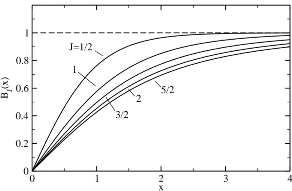
Figure 8.3: Plot of the Brillouin function BJ(x)for various values of the spin J (the total
angular momentum).
Here n is Jz = −J, . . . , J and En is our energy spacing g(JLS)µ0µBHJz. Defining η =
g(JLS)µBB)/(kBT) (i.e. the fraction of magnetic versus thermal energy), the partition
function becomes Z = J X Jz=−J e−ηJz = e −ηJ −eη(J+1) 1−eη = e− η(J+1/2) −eη(J+1/2) e−η/2 −eη/2 = sinh [(J + 1/2)η] sinh [η/2] . (8.37) With this, one finds for the magnetization
M(T) = − 1 µ0V ∂F ∂H = − 1 µ0V ∂(−kBTlnZ) ∂H (8.38) = kBT µ0V ∂ ∂H [ln (sinh[(J + 1/2)η])−ln (sinh[η/2])] = g(JLS)µBJ V BJ(η), where in the last step, we have defined the so-called Brillouin function
BJ(η) = 1 J (J+ 1 2) coth (J +1 2)η/J −12cothh η 2J i . (8.39) As shown in Fig. 8.3, BJ →1 for η ≫1, in which case eq. (8.38) simply tells us that all
atomic magnets with momentum matom, cf. eq. (8.34), have aligned to the external field,
and the magnetization reaches its maximum value of M = matom/V, i.e. the magnetic
We had, however, discussed above, that η = (g(JLS)µBB)/(kBT) will be much smaller
than unity for normal field strengths. At all but the lowest temperatures, the other limit for the Brillouin function, i.e. BJ(η → 0), will therefore be much more relevant. This
small η-expansion is
BJ(η≪1) ≈
J + 1
3 η + O(η
3) . (8.40)
In this limit, we finally obtain for the paramagnetic susceptibility χmag,para(T) = ∂M ∂H = µoµ2Bg(JLS)2J(J + 1) 3V kB 1 T = C T . (8.41)
With χmag,para>0, we have now confirmed our previous hypothesis, that the first term in
eq. (8.26) gives a paramagnetic contribution. The inverse dependence of the susceptibility on temperature is known as Curie’s law, χmag,para = C
Curie/T with CCurie the Curie
con-stant. Such a dependence is characteristic for a system with “molecular magnets” whose alignment is favored by the applied field, and that is opposed by thermal disorder. Again, we see that the first-principles derivation allows not only shows us the validity range of this empirical law (remember that it only holds in the small η-limit), but also provides the proportionality constant in terms of fundamental properties of the system.
To make a quick size estimate, we take the volume of atomic order (V ∼Å3) to find
χmag,para ∼ 10−2 at room temperature. The paramagnetic contribution is thus orders of
magnitude larger than the diamagnetic or the Van Vleck one, even at room temperature. Nevertheless, withχmag,para ≪1it is still small compared to electric susceptibilities, which
are of the order of unity. We will discuss the consequences of this in section 8.3.4, but before we have to evaluate a last remaining, additional source of magnetic behavior in metals, i.e. the free electrons.
8.3.3
Susceptibility of the free electron gas
Having determined the magnetic properties of electrons bound to ions, it is valuable to also consider the opposite extreme and examine their properties as they move nearly freely in a metal. There are again essentially two major terms in the response of free fermions to an external magnetic field. One results from the “alignment” of spins (which is a rough way of visualizing the quantum mechanical action of the field on the spins) and is calledPauli paramagnetism. The other arises from the orbital moments created by induced circular
motions of the electrons. It thus tends to screen the exterior field and is known asLandau diamagnetism.
Let us first try to analyze the origin of Pauli paramagnetism and examine its order of magnitude like we have also done for all atomic magnetic effects. For this we consider again the free electron gas, i.e. N non-interacting electrons in a volume V. In chapter 2 we had already derived the density of states (DOS) per volume
N(ǫ) = V 2π2 2me ~2 3/2 √ ǫ . (8.42)
In the electronic ground state, all states are filled following the Fermi-distribution N
V =
Z ∞
0
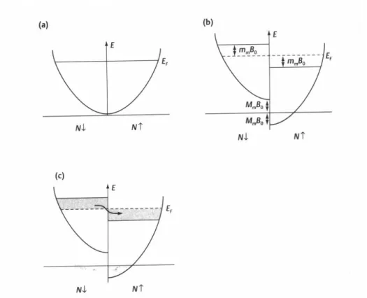
Figure 8.4: Free electron density of states and the effect of an external field: N↑corresponds to the number of electrons with spins aligned parallel and N↓ antiparallel to the z-axis. (a) No magnetic field, (b) a magnetic field, µ0H0 is applied along the z-direction, (c) as
a result of (b) some electrons with spins antiparallel to the field (shaded region on left) change their spin and move into available lower energy states with spins aligned parallel to the field.
The electron density N/V uniquely characterizes our electron gas. For sufficiently low temperatures, the Fermi-distribution can be approximated by a step function, so that all states up to the Fermi level are occupied. This Fermi level is conveniently expressed in terms of the Wigner-Seitz radius rs that we had already defined in chapter 6
ǫF = 50.1 eV rs aB 2 . (8.44)
The DOS at the Fermi level can then also be expressed in terms of rs
N(ǫF) = 1 20.7 eV rs aB −1 . (8.45)
Up to now we have not explicitly considered the spin degree of freedom, which leads to the double occupation of each electronic state with a spin up and a spin down electron. Such an explicit consideration becomes necessary, however, when we now include an external field. This is accomplished by defining spin up and spin down DOSs, N↑ and N↓, in
analogy to the spin-unresolved case. In the absence of a magnetic field, the ground state of the free electron gas has an equal number of spin-up and spin-down electrons, and the
degenerate spin-DOS are therefore simply half-copies of the original total DOS defined in eq. (8.42)
N↑(ǫ) = N↓(ǫ) = 1
2N(ǫ) , (8.46)
cf. the graphical representation in Fig. 8.4a.
An external field µ0H will now interact differently with spin up and spin down states.
Since the electron gas is fully isotropic we can always choose the spin axis that defines up and down spins to go along the direction of the applied field, and thus reduce the problem to one dimension. If we focus only on the interaction of the spin with the field and neglect the orbital response for the moment, the effect boils down to an equivalent of eq. (8.22), i.e. we have
∆Hspin(H) = µ0µBg0H·s = +µ0µBH (for spin up) (8.47)
= −µ0µBH (for spin down) (8.48)
where we have again approximated the electronic g-factorg0 by 2. The effect is therefore
simply to shift spin up electrons relative to spin down electrons. This can be expressed via the spin DOSs
N↑(ǫ) = 1
2N(ǫ−µ0µBH) (8.49)
N↓(ǫ) = 1
2N(ǫ+µ0µBH) , (8.50) or again graphically by shifting the two parabolas with respect to each other as shown in Fig. 8.4b. If we now fill the electronic states according to the Fermi-distribution, a different number of up and down electrons results and our electron gas exhibits a net magnetization due to the applied field. Since the states aligned parallel to the field are favored, the magnetization will enhance the exterior field and a paramagnetic contribution results.
For T ≈0 both parabolas are essentially filled up to a sharp energy, and the net magne-tization is simply given by the dark grey shaded region in Fig. 8.4c. Even for fields of the order of Tesla, the energetic shift of the states is µBµ0H ∼10−4eV, i.e. small on the scale
of electronic energies. The shaded region representing our net magnetization can therefore be approximated by a simple rectangle of heightµ0µBH and width 12N(ǫF), i.e. the Fermi
level DOS of the unperturbed system without applied field. We then have N↑ = N
2 + 1
2N(ǫF)µ0µBH (8.51) up electrons per volume and
N↓ = N 2 −
1
2N(ǫF)µ0µBH (8.52) down electrons per volume. Since each electron contributes a magnetic moment of µB to
the magnetization, we have
(remember that the magnetization was the dipole magnetic density, and can in our uniform system therefore be written as dipole moment per electron times DOS). This then yields the susceptibility
χmag,Pauli = ∂M
∂H = µ0µ
2
BN(ǫF) . (8.54)
Using eq. (8.45) for the Fermi level DOS of the free electron gas, this can be rewritten as function of the Wigner-Seitz radius rs
χmag,Pauli = 10−6 2.59 rs/aB . (8.55)
Recalling that the Wigner-Seitz radius of most metals is of the order of 3-5aB, we find
that the Pauli paramagnetic contribution (χmag,Pauli > 0) of a free electron gas is small.
In fact, as small as the diamagnetic susceptibility of atoms, and therefore much smaller than the paramagnetic susceptibility of atoms. For magnetic atoms in a material thermal disorder at finite temperatures prevents their complete alignment to an external field and therefore keeps the magnetism small. For an electron gas, on the other hand, it is the Pauli exclusion principle that opposes such an alignment by forcing the electrons to occupy energetically higher lying states when aligned. For the same reason, Pauli paramagnetism does not show the linear temperature dependence we observed in Curie’s law in eq. (8.41). The characteristic temperature for the electron gas is the Fermi temperature. One could therefore cast the Pauli susceptibility into Curie form, but with a fixed temperature of order TF playing the role of T. Since TF ≫ T, the Pauli susceptibility is then hundreds
of times smaller and almost always completely negligible.
Turning to Landau diamagnetism, we note that its calculation would require solving the full quantum mechanical free electron problem along similar lines as done in the last section for atoms. The field-dependent Hamilton operator would then also produce a term that screens the applied field. Taking the second derivative of the resulting total energy with respect to H, one would obtain for the diamagnetic susceptibility
χmag,Landau = −1 3χ
mag,Pauli , (8.56)
i.e. another term that is as vanishingly small as the paramagnetic response of the free electron gas. Because this term is so small and the derivation does not yield new insight compared to the one already undertaken for the atomic case, we refer to e.g. the book by M.P. Marder, Condensed Matter Physics (Wiley, 2000) for a proper derivation of this
result.
8.3.4
Atomic magnetism in solids
So far we have taken the tight-binding viewpoint of a material being an ensemble of atoms to understand its magnetic behavior. That is why we first addressed the magnetic properties of isolated atoms and ions. As an additional source of magnetism in solids we looked at free (delocalized) electrons. In both cases we found two major sources of magnetism: a paramagnetic one resulting from the alignment of existing “microscopic magnets” (either total angular momentum in the case of atoms, or spin in case of free electrons), and a diamagnetic one arising from induction currents trying to screen the external field.
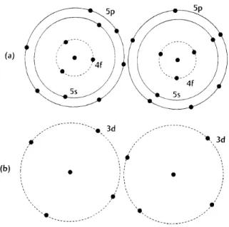
Figure 8.5: (a) In rare earth metal atoms the incomplete 4f electronic subshell is located inside the 5s and 5p subshells, so that the 4f electrons are not strongly affected by neighboring atoms. (b) In transition metal atoms, e.g. the iron group, the3d electrons are the outermost electrons, and therefore interact strongly with other nearby atoms.
• Atoms (bound electrons):
- Paramagnetism χmag,para ≈1/T ∼10−2(RT) ∆Epara
0 ∼10−4eV
- Larmor diamagnetism χmag,dia ≈const.∼ −10−4 ∆Edia
0 ∼10−9eV
• Free electrons:
- Pauli paramagnetism χmag,Pauli ≈const.∼10−6 ∆EPauli
0 ∼10−4eV
- Landau diamagnetism χmag,Landau ≈const.∼ −10−6 ∆ELandau
0 ∼10−4eV
If the coupling between the different sources of magnetism is small, the magnetic behavior of the material would simply be a superposition of all relevant terms. For insulators this would imply, for example, that the magnetic moment of each atom/ion does not change appreciably when transfered to the material and the total susceptibility would be just the sum of all atomic susceptibilities. And this is indeed primarily what one finds when going through the periodic table:
Insulators:WhenJ = 0, the paramagnetic contribution vanishes. If in additionL=S = 0 (closed-shell), the response is purely diamagnetic as in the case of noble gas solids or simple ionic crystals like the alkali halides (recall from the discussion on cohesion that the latter can be viewed as closed-shell systems!) or certain molecule (e.g. H2O) and molecular
crystals. Otherwise, the response is a balance between Van Vleck paramagnetism and Larmor diamagnetism. In all cases, the effects are small and the results from the theoretical derivation presented in the previous section are in excellent quantitative agreement with experiment.
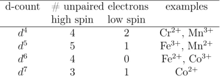
d-count # unpaired electrons examples high spin low spin
d4 4 2 Cr2+, Mn3+
d5 5 1 Fe3+, Mn2+
d6 4 0 Fe2+, Co3+
d7 3 1 Co2+
Table 8.3: High and low spin octahedral transition metal complexes.
More frequent is the situation J 6= 0, in which the response is dominated by the param-agnetic term. This is the case, when the material contains rare earth (RE) or transition metal (TM) ions (with partially filled f or d shells, respectively). These systems indeed obey Curie’s law, i.e. they exhibit susceptibilities that scale inversely with temperature. For the rare earths, even the magnitude of the measured Curie constant corresponds very well to the theoretical one given by eq. (8.41). For TM ions in insulating solids, on the other hand, the measured Curie constant can only be understood by assuming L = 0, whileS is still given by Hund’s rules. This is referred to asquenching of the orbital angular momentum and is caused by a general phenomenon known as crystal field splitting. As
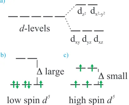
illustrated by Fig. 8.5, the f orbitals of a RE atom are located deep inside the filled s and p shells and are therefore not significantly affected by the crystalline environment. On the contrary, the d shells of a TM atom belong to the outermost valence shells and are particularly sensitive to the environment. The crystal field lifts the 5-fold degeneracy of the TM d-states, as shown for an octahedral environment in Fig. 8.6a). Hund’s rules are then in competition with the energy scale of the d-state splitting. If the energy sepa-ration is large only the three lowest states can be filled and Hund’s rules give a low spin configuration with weak diamagnetism (Fig. 8.6b) ). If the energy separation is small, Hund’s rules can still be applied to all 5 states and a high spin situation with strong paramagnetism emerges (Fig. 8.6c) ). The important thing to notice is, that although the solid perturbs the magnitude of the “microscopic magnet” connected with the partially filled shell, all individual moments inside the material are still virtually decoupled from each other (i.e. the magnetic moment in the material is that of an atom that has simply adapted to a new symmetry situation). This is why Curie’s law is still valid, but the magnetic moment becomes an effective magnetic moment that depends on the crystalline environment. Table 8.3 summarizes the configurations for some transition metal ions in an octahedral environment.
Semiconductors: Covalent materials have only partially filled shells, so they could be expected to have a finite magnetic moment. However, covalent bonds form through a pair of electrons with opposite spin, and hence the net orbital angular momentum is zero. Co-valent materials like Si (when they are not doped!!) exhibit therefore only a vanishingly small diamagnetic response. Dilute magnetic semiconductors, i.e. semiconductors doped with transition metal atoms, hold the promise to combine the powerful world of semicon-ductors with magnetism. However, questions like how pronounced the magnetism is and if room temperature magnetism can be achieved are still heavily debated and subject of an active research field.
Metals: In metals, the delocalized electrons add a new contribution to the magnetic be-havior. In simple metals like the alkalis, this new contribution is in fact the only remaining
Figure 8.6: Effect of octahedral environment on transition metal ion with 5 electrons (d5):
a) the degenerate levels split into two groups, b) for large energy separation a low spin and for small energy separation a high spin configuration c) might be favorable.
one. As discussed in the chapter on cohesion, such metals can be viewed as closed-shell ion cores and a free electron glue formed from the valence electrons. The closed-shell ion cores have J = L =S = 0 and exhibit therefore only a negligible diamagnetic response. The magnetic behavior is then dominated by the Pauli paramagnetism of the conduction electrons. Measured susceptibilities are indeed of the order as expected from eq. (8.55), and the quantitative differences arise from the exchange-correlation effects that were not treated in our free electron model. More to come on metals below...
8.4
Magnetic order: Permanent magnets
The essence of the theory we have developed up to now is, that the magnetic properties of the majority of materials can be described entirely with the picture of atomic- and free-electron magnetism. In all cases, the paramagnetic or diamagnetic response is very small, at least when compared to electric susceptibilities, which are of the order of unity. This, by the way, is also the reason why typically only electric effects are discussed in the context of interactions with electromagnetic fields. At this stage, we could therefore close the chapter on magnetism of solids as something really unimportant, if it was not for a few elemental and compound materials (formed of or containing transition metal or rare earth atoms) that exhibit a completely different magnetic behavior: enormous susceptibilities and a magnetization that does not vanish when the external field is removed. Since such so-called ferromagnetic effects are not captured by the hitherto developed theory, they
must originate from a strong coupling of the individual magnetic moments, which is what we will consider next.
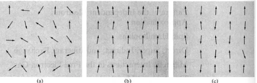
Figure 8.7: Schematic illustration of the distribution of directions of the local magnetic moments connected to “individual magnets” in a material. (a) random thermal disorder in a paramagnetic solid with insignificant magnetic interactions, (b) complete alignment either in a paramagnetic solid due to a strong external field or in a ferromagnetic solid below its critical temperature as a result of magnetic interactions. (c) Example of anti-ferromagnetic ordering below the critical temperature.
8.4.1
Ferro-, antiferro- and ferrimagnetism
The simple theory of paramagnetism in materials assumes that the individual magnetic moments (ionic shells of non-zero angular momentum in insulators or the conduction elec-trons in simple metals) do not interact with one another. In the absence of an external field, the individual magnetic moments are then thermally disordered at any finite tem-perature, i.e. they point in random directions yielding a zero net moment for the solid as a whole, cf. Fig. 8.7a. In such cases, an alignment can only be caused by an applied external field, which leads to an ordering of all magnetic moments at sufficiently low temperatures as schematically shown in Fig. 8.7b. However, a similar effect could also be obtained by coupling the different magnetic moments, i.e. by having an interaction that would favor a parallel alignment for example. Already quite short-ranged interactions, for example only between nearest neighbors, would already lead to an ordered structure as shown in Fig. 8.7b. Such interactions are often generically denoted as magnetic interaction, although
this should not be misunderstood as implying that the source of interaction is really mag-netic in nature (e.g. a magmag-netic dipole-dipole interaction, which in fact is not the reason for the ordering as we will see below).
Materials that exhibit an ordered magnetic structure in the absence of an applied external field are called ferromagnets(or permanent magnets), and their resulting (often
nonvan-ishing) magnetic moment is known as spontaneous magnetization Ms. The complexity of
the possible magnetically ordered states exceeds the simple parallel alignment case shown in Fig. 8.7b by far. In another common case the individual local moments sum to zero, and no spontaneous magnetization is present to reveal the microscopic ordering. Such mag-netically ordered states are classified as antiferromagnetic and one possible realization is
shown in Fig. 8.7c. If magnetic moments of different magnitude are present in the material, and not all local moments have a positive component along the direction of spontaneous magnetization, one talks about ferrimagnets (Ms 6= 0). Fig. 8.8 shows a few examples of
possible ordered structures. However, the complexity of possible magnetic structures is so large that some of them do not rigorously fall into any of the three categories. Those structures are well beyond the scope of this lecture and will not be covered here.
Figure 8.8: Typical magnetic orders in a simple linear array of spins. (a) ferromagnetic, (b) antiferromagnetic, and (c) ferrimagnetic.
Figure 8.9: Typical temperature dependence of the magnetizationMs, the specific heatcV
and the zero-field susceptibility χo of a ferromagnet. The temperature scale is normalized
to the critical (Curie) temperature Tc.
8.4.2
Interaction versus thermal disorder: Curie-Weiss law
Even in permanent magnets, the magnetic order does not usually prevail at all tempera-tures. Above a critical temperature Tc, the thermal energy can overcome the interaction
induced order. The magnetic order vanishes and the material (often) behaves like a simple paramagnet. In ferromagnets,Tc is known as theCurie temperature, and in
antiferromag-nets as Néel temperature (sometimes denoted TN). Note that Tc may depend strongly
on the applied field (both in strength and direction!). If the external field is parallel to the direction of spontaneous magnetization, Tc typically increases with increasing
exter-nal field, since both ordering tendencies support each other. For other field directions, a range of complex phenomena can arise as a result of the competition between both ordering tendencies.
At the moment we are, however, more interested in the ferromagnetic properties of materi-als in the absence of external fields, i.e. the existence of a finite spontaneous magnetization. The gradual loss of order with increasing temperature is reflected in the continuous drop of Ms(T) as illustrated in Fig. 8.9. Just below Tc, a power law dependence is typically
observed
Ms(T) ∼ (Tc−T)β (for T →Tc−) , (8.57)
with a critical exponent β somewhere around 1/3. Coming from the high temperature side, the onset of ordering also appears in the zero-field susceptibility, which is found to diverge as T approaches Tc
χo(T) = χ(T)|B=0 ∼ (T −Tc)−γ (for T →Tc+) , (8.58)
with γ around 4/3. This behavior already indicates that the material experiences dra-matic changes at the critical temperature, which is also reflected by a divergence in other fundamental quantities like the zero-field specific heat
¯
ms (in µB) matom (in µB) Tc (in K) Θc (in K)
Fe 2.2 6 (4) 1043 1100 Co 1.7 6 (3) 1394 1415 Ni 0.6 5 (2) 628 650 Eu 7.1 7 289 108 Gd 8.0 8 302 289 Dy 10.6 10 85 157
Table 8.4: Magnetic quantities of some elemental ferromagnets: The saturation magneti-zation at T = 0K is given in form of the average magnetic momentm¯s per atom and the
critical temperatureTc and the Curie-Weiss temperatureΘc are given in K. For
compar-ison also the magnetic moment matom of the corresponding isolated atoms is listed (the
values in brackets are for the case of orbital angular momentum quenching).
with α around 0.1. The divergence is connected to the onset of long-range order (align-ment), which sets in more less suddenly at the critical temperature resulting in a second order phase transition. The actual transition is difficult to describe theoretically and the-ories are therefore often judged by how well (or badly) they reproduce the experimentally measured critical exponents α, β and γ.
Above the critical temperature, the properties of magnetic materials often become “more normal”. In particular, for T ≫ Tc, one usually finds a simple paramagnetic behavior,
with a susceptibility that obeys the so-called Curie-Weiss law, cf. Fig. 8.9,
χo(T) ∼ (T −Θc)−1 (for T ≫Tc) . (8.60)
Θc is called the Curie-Weiss temperature. Since γ in eq. (8.58) is almost never exactly
equal to 1, Θc does not necessarily coincide with the Curie temperature Tc. This can,
for example, be seen in Table 8.4, where also the saturated values for the spontaneous magnetization at T →0K are listed.
In theoretical studies one typically converts this measured Ms(T →0 K) directly into an
average magnetic momentm¯s per atom (in units ofµB) by simply dividing by the atomic
density in the material. In this way, we can compare directly with the corresponding values for the isolated atoms, obtained asmatom =g(JLS)µBJ, cf. eq. (8.34). As apparent from
Table 8.4, the two values agree very well for the rare earth metals, but differ substantially for the transition metals. Recalling the discussion on the quenching of the orbital angular momentum of TM atoms immersed in insulating materials in section 8.3.4, we could once again try to ascribe this difference to the symmetry lowering of interactingdorbitals in the material. Yet, even using L= 0 (and thus J =S, g(JLS) = 2), the agreement does not become much better, cf. Table 8.4. In the RE ferromagnets, the saturation magnetization appears to be a result of the perfect alignment of atomic magnetic moments that are not strongly affected by the presence of the surrounding material. The TM ferromagnets (Fe, Co, Ni), on the other hand, exhibit a much more complicated magnetic structure that is not well described by the magnetic behavior of the individual atoms.
As a first summary of our discussion on ferromagnetism (or ordered magnetic states in general) we are therefore led to conclude that it must arise out of an (yet unspecified) interaction between magnetic moments. This interaction produces an alignment of the magnetic moments, and subsequently a large net magnetization that prevails even in the
absence of an external field. This means we are certainly outside the linear response regime that has been our basis for developing the dia- and paramagnetic theories in the first sec-tions of this chapter. With regard to the alignment, the interaction seems to have the same effect as an applied field acting on a paramagnet, which explains the similarity between the Curie-Weiss and the Curie law of paramagnetic solids: Interaction and external field favor alignment, and are opposed by thermal disorder. Below the critical temperature the alignment is perfect, and far above Tc the competition between alignment and disorder is
equivalent to the situation in a paramagnet (just the origin of the temperature scale has shifted).
Sources for the interacting magnetic moments can be either delocalized electrons (Pauli paramagnetism) or partially filled atomic shells (Paramagnetism). This makes it plausi-ble why ferromagnetism is a phenomenon specific to only some metals, and in particular metals with a high magnetic moment that arises from partially filled d or f shells (i.e. transition metals, rare earths, as well as their compounds). However, we cannot yet explain why only some and not all TMs and REs exhibit ferromagnetic behavior. The comparison between the measured values of the spontaneous magnetization and the atomic magnetic moments suggests that ferromagnetism in RE metals can be understood as the coupling of localized magnetic moments (due to the inert partially filledf shells). The situation is more complicated for TM ferromagnets, where the picture of a simple coupling between atomic-like moments fails. We will see below that this so-called itinerant ferromagnetism
arises out of a subtle mixture of delocalized s electrons and the more localized, but nev-ertheless not inert dorbitals.
8.4.3
Phenomenological theories of ferromagnetism
After this first overview of phenomena arising out of magnetic order, let us now try to establish a proper theoretical understanding. Unfortunately, the theory of ferromagnetism is one of the less well developed of the fundamental theories in solid state physics (a bit better for the localized ferromagnetism of the REs, worse for the itinerant ferromagnetism of the TMs). The complex interplay of single particle and many-body effects, as well as collective effects and strong local coupling makes it difficult to break the topic down into simple models appropriate for an introductory level lecture. We will therefore not be able to present and discuss a full-blownab initiotheory like in the preceding chapters. Instead
we will first consider simple phenomenological theories and refine them later, when needed. This will enable us to address some of the fundamental questions that are not amenable to phenomenological theories (like the source of the magnetic interaction).
8.4.3.1 Molecular (mean) field theory
The simplest phenomenological theory of ferromagnetism is themolecular field theorydue
to Weiss (1906). We had seen in the preceding section that the effect of the interaction between the discrete magnetic moments in a material is very similar to that of an applied external field (leading to alignment). For each magnetic moment, the net effect of the interaction with all other moments can therefore be thought of as a kind of internal field created by all other moments (and the magnetic moment itself). In this way we average over all interactions and condenses them into one effective field, i.e. molecular field theory is a typical representative of a mean field theory. Since this effective internal, or so-called
molecular field corresponds to an average over all interactions, it is reasonable to assume
that it will scale with M, i.e. the overall magnetization (density of magnetic moments). Without specifying the microscopic origin of the magnetic interaction and the resulting field, the ansatz of Weiss was to simply postulate a linear scaling with M
Hmol = µoλM , (8.61)
where λ is the so-called molecular field constant. This leads to an effective field
Heff = H+Hmol = H+µoλM , (8.62)
For simplicity, we will consider only the case of an isotropic material, so that the internal and the external point in the same direction, allowing us to write all formulae as scalar relations.
Recalling the magnetization of paramagnetic spins (Eq. 8.38) M0(T) = g(JLS)µBJ V BJ(η) withη ∼ H T (8.63) we obtain M(T) =M0 Hef f T →M0 λM T (8.64) when the external field is switched off (H=0). We now ask the question if such a field can exist without an external field? Since M appears on the left and on the right hand side of the equation we perform a graphic solution. We set x= TλM(T), which results in
M0(x) =
T
λx . (8.65)
The graphic solution is show in Fig. 8.10 and tells us that the slop of M0(0K) has to be
larger than T
λ. If this condition is fulfilled a ferromagnetic solution of our paramagnetic
mean field model is obtained, although at this point we have no microscopic understanding of λ.
For the mean-field susceptibility we then obtain withH(T) =M0(Hef fT )
χ= ∂M0 ∂H = ∂M0 ∂Hef f ∂Hef f ∂H = C T 1 + ∂M ∂H = C T (1 +λχ) (8.66) where we have used that for our paramagnet ∂M0
∂Hef f is just Curie’s law. Solving Eq. 8.66
for χ gives the Curie-Weiss law
χ= C
T −λC ∼(T −Θc)
−1
. (8.67)
Θcis the Curie-Weiss temperature. The form of the Curie-Weiss law is compatible with an
effective molecular field that scales linearly with the magnetization. Given the experimen-tal observation of Curie-Weiss like scaling, the mean field ansatz of Weiss seems therefore reasonable. However, we can already see that this simple theory fails, as it predicts an inverse scaling with temperature for all T > Tc, i.e. within molecular field theoryΘc =Tc
and γ = 1 at variance with experiment. The exponent of 1, by the way, is characteristic for any mean field theory.
Figure 8.10: Graphical solution of equation 8.64.
Given the qualitative plausibility of the theory, let us nevertheless use it to derive a first order of magnitude estimate for this (yet unspecified) molecular field. This phenomeno-logical consideration therefore follows the reverse logic to the ab initio one we prefer. In
the latter, we would have analyzed the microscopic origin of the magnetic interaction and derived the molecular field as a suitable average, which in turn would have brought us into a position to predict materials’ properties like the saturation magnetization and the crit-ical temperature. Now, we do the opposite: We will use the experimentally known values ofMs and Tc to obtain a first estimate of the size of the molecular field, which might help
us lateron to identify the microscopic origin of the magnetic interactions (about which we still do not know anything). For the estimate, recall that the Curie constant C was given by eq. (8.38) as C = Nµoµ 2 Bg(JLS)2J(J + 1) 3kBV ≈ N V µom2atom 3kB , (8.68)
where we have exploited that J(J+ 1)∼J2, allowing us to identify the atomic magnetic
moment matom =µBg(JLS)J. With this, it is straightforward to arrive at the following
estimate of the molecular field at T = 0K, Bmol(0 K) = µoλMs(0 K) =µo Tc C N V m¯s ≈ 3kBTcm¯s m2 atom (8.69) When discussing the content of Table 8.4 we had already seen that for most ferromagnets, matom is at least of the same order of m¯s, so that plugging in the numerical constants we
arrive at the following order of magnitude estimate Bmol ∼ [5Tc in K]
[matom inµB]
Looking at the values listed in Table 8.4, one realizes that molecular fields are of the order of some103Tesla, which is at least one order of magnitude more than the strongest
magnetic fields that can currently be produced in the laboratory. As take-home message we therefore keep in mind that the magnetic interactions must be quite strong to yield such a high internal molecular field.
Molecular field theory can also be employed to understand the temperature behavior of the zero-field spontaneous magnetization. As shown in Fig. 8.9 Ms(T) decays smoothly from
its saturation value at T = 0K to zero at the critical temperature. Since the molecular field produced by the magnetic interaction is indistinguishable from an applied external one, the variation of Ms(T) must be equivalent to the one of a paramagnet, only with
the external field replaced by the molecular one. Using the results from section 8.3.2 for atomic paramagnetism, we therefore obtain directly a behavior equivalent to eq. (8.38)
Ms(T) = Ms(0 K) BJ g(JLS)µBBmol kBT , (8.71)
i.e. the temperature dependence is entirely given by the Brillouin function defined in eq. (8.39).BJ(η), in fact, exhibits exactly the behavior we just discussed: it decays smoothly to
zero as sketched in Fig. 8.9. Similar to the reproduction of the Curie-Weiss law, mean field theory provides us therefore with a simple rationalization of the observed phenomenon, but fails again on a quantitative level (and also does not tell us anything about the underlying microscopic mechanism). The functional dependence of Ms(T) in both limits
T →0K and T →T−
c is incorrect, with e.g.
Ms(T →Tc−) ∼ (Tc−T)1/2 (8.72)
and thus β = 1/2 instead of the observed values around 1/3. In the low temperature limit, the Brillouin function decays exponentially fast, which is also in gross disagreement with the experimentally observedT3/2 behavior (known asBlochT3/2 law). The failure to
predict the correct critical exponents is a general feature mean field theories that cannot account for the fluctuations connected with phase transitions. The wrong low temperature limit, on the other hand, is due to the non-existence of a particular set of low-energy excitations called spin-waves (or magnons), a point that we will come back to later. 8.4.3.2 Heisenberg and Ising Hamiltonian
Another class of phenomenological theories is calledspin Hamiltonians. They are based on
the hypothesis that magnetic order is due to the coupling between discrete microscopic magnetic moments. If these microscopic moments are, for example, connected to the partially filled f-shells of RE atoms, one can replace the material by a discrete lattice model, in which each sitei has a magnetic momentmi. A coupling between two different sites i and j in the lattice can then be described by a term
Hi,jcoupling = −Jij µ2
B
mi·mj , (8.73)
whereJij is known as the exchange coupling constant between the two sites (unit: eV). In
principle, the coupling can take any value between−Jijmimj/µ2B(parallel (ferromagnetic)
Figure 8.11: Schematic illustrations of possible coupling mechanisms between localized magnetic moments: (a) direct exchange between neighboring atoms, (b) superexchange mediated by non-magnetic ions, and (c) indirect exchange mediated by conduction elec-trons.
the relative orientation of the two moment vectors. Note that this simplified interaction has no explicit spatial dependence anymore. If this is required (e.g. in a non-isotropic crystal with a preferred magnetization axis), additional terms need to be added to the Hamiltonian.
Applying this coupling to the whole material, we first have to decide which lattice sites to couple. Since we are now dealing with a phenomenological theory we have no rigorous guidelines that would tell us which interactions are important. Instead, we have to choose the interactions (e.g. between nearest neighbors or up to next-nearest neighbors) and their strengthsJij. Later, after we have solved the model, we can revisit these assumptions and
see if they were justified. We can also use experimental (or first principles) data to fit the Jij’s and hope to extract microscopic information. Often our choice is guided by intuition
concerning the microscopic origin of the coupling. For the localized ferromagnetism of the rare earths one typically assumes a short-ranged interaction, which could either be between neighboring atoms (direct exchange) or reach across non-magnetic atoms in more
complex structures (superexchange). As illustrated in Fig. 8.11 this conveys the idea that
the interaction arises out of an overlap of electronic wavefunctions. Alternatively, one could also think of an interaction mediated by the glue of conduction electrons (indirect exchange), cf. Fig. 8.11c. However, without a proper microscopic theory it is difficult to
distinguish between these different possibilities.