C H A P T E R
14
Bootstrap Methods
and Permutation Tests*
14.1 The Bootstrap Idea
14.2 First Steps in Usingthe Bootstrap
14.3 How Accurate Is a Bootstrap Distribution?
14.4 Bootstrap Confidence Intervals
14.5 Significance Testing Using
Permutation Tests
*This chapter was written by Tim Hesterberg, David S. Moore, Shaun Monaghan, Ashley Clip-son, and Rachel Epstein, with support from the National Science Foundation under grant DMI-0078706. We thank Bob Thurman, Richard Heiberger, Laura Chihara, Tom Moore, and Gudmund Iversen for helpful comments on an earlier version.
Introduction
The continuing revolution in computing is having a dramatic influence on statistics. Exploratory analysis of data becomes easier as graphs and calcula-tions are automated. Statistical study of very large and very complex data sets becomes feasible. Another impact of fast and cheap computing is less obvious: new methods that apply previously unthinkable amounts of computation to small sets of data to produce confidence intervals and tests of significance in settings that don’t meet the conditions for safe application of the usual meth-ods of inference.
The most common methods for inference about means based on a single sample, matched pairs, or two independent samples are the t procedures de-scribed in Chapter 7. For relationships between quantitative variables, we use other t tests and intervals in the correlation and regression setting (Chap-ter 10). Chap(Chap-ters 11, 12, and 13 present inference procedures for more elab-orate settings. All of these methods rest on the use of normal distributions for data. No data are exactly normal. The t procedures are useful in prac-tice because they are robust, quite insensitive to deviations from normality in the data. Nonetheless, we cannot use t confidence intervals and tests if the data are strongly skewed, unless our samples are quite large. Inference about spread based on normal distributions is not robust and is therefore of little use in practice. Finally, what should we do if we are interested in, say, a ratio of means, such as the ratio of average men’s salary to average women’s salary? There is no simple traditional inference method for this setting.
The methods of this chapter—bootstrap confidence intervals and permuta-tion tests—apply computing power to relax some of the condipermuta-tions needed for traditional inference and to do inference in new settings. The big ideas of sta-tistical inference remain the same. The fundamental reasoning is still based on asking, “What would happen if we applied this method many times?” An-swers to this question are still given by confidence levels and P-values based on the sampling distributions of statistics. The most important requirement for trustworthy conclusions about a population is still that our data can be regarded as random samples from the population—not even the computer can rescue voluntary response samples or confounded experiments. But the new methods set us free from the need for normal data or large samples. They also set us free from formulas. They work the same way (without formulas) for many different statistics in many different settings. They can, with suffi-cient computing power, give results that are more accurate than those from traditional methods. What is more, bootstrap intervals and permutation tests are conceptually simpler than confidence intervals and tests based on nor-mal distributions because they appeal directly to the basis of all inference: the sampling distribution that shows what would happen if we took very many samples under the same conditions.
The new methods do have limitations, some of which we will illustrate. But their effectiveness and range of use are so great that they are rapidly be-coming the preferred way to do statistical inference. This is already true in high-stakes situations such as legal cases and clinical trials.
Software
Bootstrapping and permutation tests are feasible in practice only with soft-ware that automates the heavy computation that these methods require. If you
are sufficiently expert, you can program at least the basic methods yourself. It is easier to use software that offers bootstrap intervals and permutation tests preprogrammed, just as most software offers the various t intervals and tests. You can expect the new methods to become gradually more common in stan-dard statistical software.
This chapter uses S-PLUS,1 the software choice of most statisticians do-ing research on resampldo-ing methods. A free version of S-PLUS is available to students. You will also need two free libraries that supplement S-PLUS: the
S+Resamplelibrary, which provides menu-driven access to the procedures de-scribed in this chapter, and theIPSdatalibrary, which contains all the data sets for this text. You can find links for downloading this software on the text Web site,www.whfreeman.com/ipsresample.
You will find that using S-PLUS is straightforward, especially if you have experience with menu-based statistical software. After launching S-PLUS, load theIPSdatalibrary. This automatically loads theS+Resamplelibrary as
well. The IPSdata menu includes a guide with brief instructions for each
procedure in this chapter. Look at this guide each time you meet something new. There is also a detailed manual for resampling under the Help menu.
The resampling methods you need are all in theResamplingsubmenu in the Statistics menu in S-PLUS. Just choose the entry in that menu that
de-scribes your setting.
S-PLUS is highly capable statistical software that can be used for every-thing in this text. If you use S-PLUS for all your work, you may want to obtain a more detailed book on S-PLUS.
14.1 The Bootstrap Idea
Here is a situation in which the new computer-intensive methods are now be-ing applied. We will use this example to introduce these methods.
E X A M P L E 1 4 . 1 telephone service. It isn’t in the public interest to have all these com-In most of the United States, many different companies offer local panies digging up streets to bury cables, so the primary local telephone company in each region must (for a fee) share its lines with its competitors. The legal term for the primary company is Incumbent Local Exchange Carrier, ILEC. The competitors are called Competing Local Exchange Carriers, or CLECs.
Verizon is the ILEC for a large area in the eastern United States. As such, it must provide repair service for the customers of the CLECs in this region. Does Verizon do repairs for CLEC customers as quickly (on the average) as for its own customers? If not, it is subject to fines. The local Public Utilities Commission requires the use of tests of significance to compare repair times for the two groups of customers.
Repair times are far from normal. Figure 14.1 shows the distribution of a ran-dom sample of 1664 repair times for Verizon’s own customers.2 The distribution has
a very long right tail. The median is 3.59 hours, but the mean is 8.41 hours and the longest repair time is 191.6 hours. We hesitate to use t procedures on such data, es-pecially as the sample sizes for CLEC customers are much smaller than for Verizon’s own customers.
0
Repair times (in hours)
z-score
Repair times (in hours)
600 500 400 300 200 100 0 50 100 150 –2 150 100 50 0 0 2 (a) (b)
FIGURE 14.1 (a) The distribution of 1664 repair times for Verizon cus-tomers. (b) Normal quantile plot of the repair times. The distribution is strongly right-skewed.
The big idea: resampling and the bootstrap distribution
Statistical inference is based on the sampling distributions of sample statis-tics. The bootstrap is first of all a way of finding the sampling distribution, at least approximately, from just one sample. Here is the procedure:Step 1: Resampling.
A sampling distribution is based on many dom samples from the population. In Example 14.1, we have just one ran-dom sample. In place of many samples from the population, create many resamples by repeatedly sampling with replacement from this one random resamplessample. Each resample is the same size as the original random sample. Sampling with replacement means that after we randomly draw an ob-sampling with
replacement servation from the original sample we put it back before drawing the next ob-servation. Think of drawing a number from a hat, then putting it back before drawing again. As a result, any number can be drawn more than once, or not at all. If we sampled without replacement, we’d get the same set of numbers we started with, though in a different order. Figure 14.2 illustrates three re-samples from a sample of six observations. In practice, we draw hundreds or thousands of resamples, not just three.
Step 2: Bootstrap distribution.
The sampling distribution of a statistic collects the values of the statistic from many samples. The bootstrap distri-bootstrapdistribution bution of a statistic collects its values from many resamples. The bootstrap distribution gives information about the sampling distribution.
THE BOOTSTRAP IDEA
The original sample represents the population from which it was drawn. So resamples from this sample represent what we would get if we took many samples from the population. The bootstrap distribu-tion of a statistic, based on many resamples, represents the sampling distribution of the statistic, based on many samples.
1.57 0.22 19.67 0.00 0.22 3.12 mean = 4.13 0.00 2.20 2.20 2.20 19.67 1.57 mean = 4.64 3.12 0.00 1.57 19.67 0.22 2.20 mean = 4.46 0.22 3.12 1.57 3.12 2.20 0.22 mean = 1.74
FIGURE 14.2 The resampling idea. The top box is a sample of sizen=6from the Verizon data. The three lower boxes are three resamples from this original sample. Some values from the original are repeated in the resamples because each resample is formed by sampling with replacement. We calculate the statistic of interest—the sample mean in this example—for the original sample and each resample.
E X A M P L E 1 4 . 2 µIn Example 14.1, we want to estimate the population mean repair time, so the statistic is the sample mean x. For our one random sample of 1664 repair times, x=8.41 hours. When we resample, we get different values of x, just as we would if we took new samples from the population of all repair times.
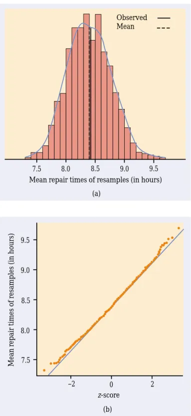
Figure 14.3 displays the bootstrap distribution of the means of 1000 resamples from the Verizon repair time data, using first a histogram and a density curve and then a normal quantile plot. The solid line in the histogram marks the mean 8.41 of the original sample, and the dashed line marks the mean of the bootstrap means. Accord-ing to the bootstrap idea, the bootstrap distribution represents the samplAccord-ing distribu-tion. Let’s compare the bootstrap distribution with what we know about the sampling distribution.
Shape:
We see that the bootstrap distribution is nearly normal. The central limit theorem says that the sampling distribution of the sample mean x is ap-proximately normal if n is large. So the bootstrap distribution shape is close to the shape we expect the sampling distribution to have.Center:
The bootstrap distribution is centered close to the mean of the orig-inal sample. That is, the mean of the bootstrap distribution has little bias as an estimator of the mean of the original sample. We know that the sampling distribution of x is centered at the population meanµ, that is, that x is an un-biased estimate ofµ. So the resampling distribution behaves (starting from the original sample) as we expect the sampling distribution to behave (start-ing from the population).Spread:
The histogram and density curve in Figure 14.3 picture the varia-tion among the resample means. We can get a numerical measure by calculat-ing their standard deviation. Because this is the standard deviation of the 1000 values of x that make up the bootstrap distribution, we call it the bootstrap bootstrapstandard error standard error of x. The numerical value is 0.367. In fact, we know that the standard deviation of x isσ /√n, whereσ is the standard deviation of indi-vidual observations in the population. Our usual estimate of this quantity is the standard error of x, s/√n, where s is the standard deviation of our one random sample. For these data, s=14.69 and
s √ n = 14.69 √ 1664 =0.360
The bootstrap standard error 0.367 agrees closely with the theory-based esti-mate 0.360.
In discussing Example 14.2, we took advantage of the fact that statistical theory tells us a great deal about the sampling distribution of the sample mean x. We found that the bootstrap distribution created by resampling matches the properties of the sampling distribution. The heavy computa-tion needed to produce the bootstrap distribucomputa-tion replaces the heavy theory (central limit theorem, mean and standard deviation of x) that tells us about the sampling distribution. The great advantage of the resampling idea is that it often works even when theory fails. Of course, theory also has its advantages: we know exactly when it works. We don’t know exactly when resampling works, so that “When can I safely bootstrap?” is a somewhat subtle issue.
7.5 8.0 8.5 9.0 9.5 Mean repair times of resamples (in hours)
(a) Observed Mean 7.5 8.0 8.5 9.0 9.5 Mean r epair times of r
esamples (in hours)
–2 0 2
z-score (b)
FIGURE 14.3 (a) The bootstrap distribution for 1000 re-sample means from the re-sample of Verizon repair times. The solid line marks the original sample mean, and the dashed line marks the average of the bootstrap means. (b) The normal quantile plot confirms that the bootstrap distribution is nearly normal in shape.
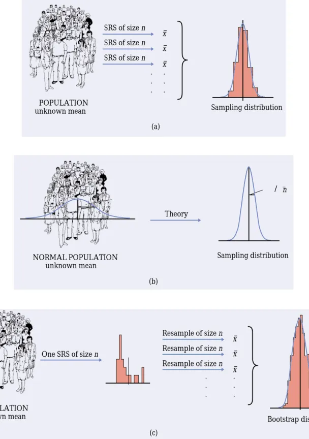
Figure 14.4 illustrates the bootstrap idea by comparing three distribu-tions. Figure 14.4(a) shows the idea of the sampling distribution of the sample mean x: take many random samples from the population, calculate the mean x for each sample, and collect these x-values into a distribution.
Figure 14.4(b) shows how traditional inference works: statistical theory tells us that if the population has a normal distribution, then the sampling dis-tribution of x is also normal. (If the population is not normal but our sample is large, appeal instead to the central limit theorem.) Ifµandσ are the mean and standard deviation of the population, the sampling distribution of x has meanµand standard deviationσ /√n. When it is available, theory is wonder-ful: we know the sampling distribution without the impractical task of actu-ally taking many samples from the population.
Figure 14.4(c) shows the bootstrap idea: we avoid the task of taking many samples from the population by instead taking many resamples from a single sample. The values of x from these resamples form the bootstrap distribution. We use the bootstrap distribution rather than theory to learn about the sam-pling distribution.
Thinking about the bootstrap idea
It might appear that resampling creates new data out of nothing. This seems suspicious. Even the name “bootstrap” comes from the impossible image of “pulling yourself up by your own bootstraps.”3 But the resampled observa-tions are not used as if they were new data. The bootstrap distribution of the resample means is used only to estimate how the sample mean of the one ac-tual sample of size 1664 would vary because of random sampling.
Using the same data for two purposes—to estimate a parameter and also to estimate the variability of the estimate—is perfectly legitimate. We do exactly this when we calculate x to estimateµand then calculate s/√n from the same data to estimate the variability of x.
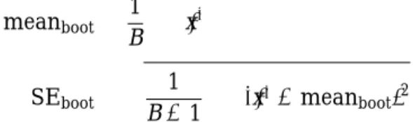
What is new? First of all, we don’t rely on the formula s/√n to estimate the standard deviation of x. Instead, we use the ordinary standard deviation of the many x-values from our many resamples.4 Suppose that we take B resamples. Call the means of these resamplesx¯∗to distinguish them from the mean x of the original sample. Find the mean and standard deviation of the x¯∗’s in the usual way. To make clear that these are the mean and standard deviation of the means of the B resamples rather than the mean x and standard deviation s of the original sample, we use a distinct notation:
meanboot= 1 B ¯ x∗ SEboot= 1 B−1 (¯x∗−meanboot)2
These formulas go all the way back to Chapter 1. Once we have the valuesx¯∗, we just ask our software for their mean and standard deviation. We will of-ten apply the bootstrap to statistics other than the sample mean. Here is the general definition.
(a) SRS of size n Sampling distribution POPULATION unknown mean x– x– · · · · · · (b) Theory Sampling distribution NORMAL POPULATION unknown mean /0_n Resample of size n Resample of size n Resample of size n (c) One SRS of size n Bootstrap distribution POPULATION unknown mean x– x– x– · · · · · ·
FIGURE 14.4 (a) The idea of the sampling distribution of the sample meanx: take very many samples, collect the x-values from each, and look at the distribution of these values. (b) The theory shortcut: if we know that the population values follow a normal distribution, theory tells us that the sampling distribution ofxis also normal. (c) The bootstrap idea: when theory fails and we can afford only one sample, that sample stands in for the population, and the distribution ofxin many resamples stands in for the sampling distribution.
BOOTSTRAP STANDARD ERROR
The bootstrap standard error SEbootof a statistic is the standard de-viation of the bootstrap distribution of that statistic.
Another thing that is new is that we don’t appeal to the central limit theo-rem or other theory to tell us that a sampling distribution is roughly normal. We look at the bootstrap distribution to see if it is roughly normal (or not). In most cases, the bootstrap distribution has approximately the same shape and spread as the sampling distribution, but it is centered at the original statistic value rather than the parameter value. The bootstrap allows us to calculate standard errors for statistics for which we don’t have formulas and to check normality for statistics that theory doesn’t easily handle.
To apply the bootstrap idea, we must start with a statistic that estimates the parameter we are interested in. We come up with a suitable statistic by appealing to another principle that we have often applied without thinking about it.
THE PLUG-IN PRINCIPLE
To estimate a parameter, a quantity that describes the population, use the statistic that is the corresponding quantity for the sample.
The plug-in principle tells us to estimate a population mean µ by the sample mean x and a population standard deviation σ by the sample stan-dard deviation s. Estimate a population median by the sample median and a population regression line by the least-squares line calculated from a sample. The bootstrap idea itself is a form of the plug-in principle: substitute the data for the population, then draw samples (resamples) to mimic the process of building a sampling distribution.
Using software
Software is essential for bootstrapping in practice. Here is an outline of the program you would write if your software can choose random samples from a set of data but does not have bootstrap functions:
Repeat 1000 times {
Draw a resample with replacement from the data. Calculate the resample mean.
Save the resample mean into a variable. }
Make a histogram and normal quantile plot of the 1000 means. Calculate the standard deviation of the 1000 means.
Number of Replications: 1000 Percentiles: 2.5% 5.0% 95.0% 97.5% mean 7.717 7.814 9.028 9.114 Summary Statistics: mean Observed 8.412 Mean 8.395 SE 0.3672 Bias –0.01698
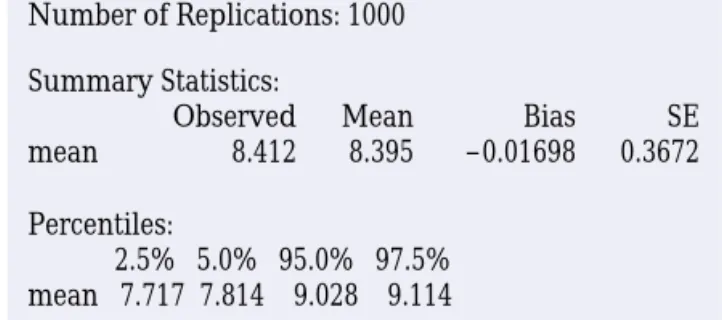
FIGURE 14.5 S-PLUS output for the Verizon data boot-strap, for Example 14.3.
E X A M P L E 1 4 . 3 times are saved as a variable, we can use menus to resample from theS-PLUS has bootstrap commands built in. If the 1664 Verizon repair data, calculate the means of the resamples, and request both graphs and printed out-put. We can also ask that the bootstrap results be saved for later access.
The graphs in Figure 14.3 are part of the S-PLUS output. Figure 14.5 shows some of the text output. TheObservedentry gives the mean x=8.412 of the original sample. Mean is the mean of the resample means, meanboot. Bias is the difference between
theMeanandObservedvalues. The bootstrap standard error is displayed underSE. The Percentilesare percentiles of the bootstrap distribution, that is, of the 1000 resample means pictured in Figure 14.3. All of these values exceptObservedwill differ a bit if you repeat 1000 resamples, because resamples are drawn at random.
SECTION 14.1
Summary
To bootstrap a statistic such as the sample mean, draw hundreds of resamples with replacement from a single original sample, calculate the statistic for each resample, and inspect the bootstrap distribution of the resampled statistics.
A bootstrap distribution approximates the sampling distribution of the statis-tic. This is an example of the plug-in principle: use a quantity based on the sample to approximate a similar quantity from the population.
A bootstrap distribution usually has approximately the same shape and spread as the sampling distribution. It is centered at the statistic (from the original sample) when the sampling distribution is centered at the parameter (of the population).
Use graphs and numerical summaries to determine whether the bootstrap dis-tribution is approximately normal and centered at the original statistic, and to get an idea of its spread. The bootstrap standard error is the standard deviation of the bootstrap distribution.
The bootstrap does not replace or add to the original data. We use the boot-strap distribution as a way to estimate the variation in a statistic based on the original data.
SECTION 14.1
Exercises
Unless an exercise instructs you otherwise, use 1000 resamples for all bootstrap exercises. S-PLUS uses 1000 resamples unless you ask for a different number. Always save your bootstrap results so that you can use them again later. 14.1 To illustrate the bootstrap procedure, let’s bootstrap a small random subset of
the Verizon data:
3.12 0.00 1.57 19.67 0.22 2.20
(a) Sample with replacement from this initial SRS by rolling a die. Rolling a 1 means select the first member of the SRS, a 2 means select the second member, and so on. (You can also use Table B of random digits, respond-ing only to digits 1 to 6.) Create 20 resamples of size n=6.
(b) Calculate the sample mean for each of the resamples.
(c) Make a stemplot of the means of the 20 resamples. This is the bootstrap distribution.
(d) Calculate the bootstrap standard error.
Inspecting the bootstrap distribution of a statistic helps us judge whether the sampling distribution of the statistic is close to normal. Bootstrap the sample mean x for each of the data sets in Exercises 14.2 to 14.5. Use a histogram and normal quantile plot to assess normality of the bootstrap distribution. On the basis of your work, do you expect the sampling distribution of x to be close to normal? Save your bootstrap results for later analysis.
14.2 The distribution of the 60 IQ test scores in Table 1.3 (page 14) is roughly mal (see Figure 1.5) and the sample size is large enough that we expect a nor-mal sampling distribution.
14.3 The distribution of the 64 amounts of oil in Exercise 1.33 (page 37) is strongly skewed, but the sample size is large enough that the central limit theorem may (or may not) result in a roughly normal sampling distribution.
14.4 The amounts of vitamin C in a random sample of 8 lots of corn soy blend (Example 7.1, page 453) are
26 31 23 22 11 22 14 31
The distribution has no outliers, but we cannot assess normality from so small a sample.
14.5 The measurements of C-reactive protein in 40 children (Exercise 7.2, page 472) are very strongly skewed. We were hesitant to use t procedures for in-ference from these data.
14.6 The “survival times” of machines before a breakdown and of cancer patients after treatment are typically strongly right-skewed. Table 1.8 (page 38) gives the survival times (in days) of 72 guinea pigs in a medical trial.5
(a) Make a histogram of the survival times. The distribution is strongly skewed.
(b) The central limit theorem says that the sampling distribution of the sample mean x becomes normal as the sample size increases. Is the sam-pling distribution roughly normal for n=72? To find out, bootstrap these data and inspect the bootstrap distribution of the mean. The central part of the distribution is close to normal. In what way do the tails depart from normality?
14.7 Here is an SRS of 20 of the guinea pig survival times from Exercise 14.6:
92 123 88 598 100 114 89 522 58 191
137 100 403 144 184 102 83 126 53 79
We expect the sampling distribution of x to be less close to normal for samples of size 20 than for samples of size 72 from a skewed distribution. These data include some extreme high outliers.
(a) Create and inspect the bootstrap distribution of the sample mean for these data. Is it less close to normal than your distribution from the previous exercise?
(b) Compare the bootstrap standard errors for your two runs. What accounts for the larger standard error for the smaller sample?
14.8 We have two ways to estimate the standard deviation of a sample mean x: use the formula s/√n for the standard error, or use the bootstrap standard error. Find the sample standard deviation s for the 20 survival times in Exercise 14.7 and use it to find the standard error s/√n of the sample mean. How closely does your result agree with the bootstrap standard error from your resam-pling in Exercise 14.7?
14.2 First Steps in Usingthe Bootstrap
To introduce the big ideas of resampling and bootstrap distributions, we stud-ied an example in which we knew quite a bit about the actual sampling dis-tribution. We saw that the bootstrap distribution agrees with the sampling distribution in shape and spread. The center of the bootstrap distribution is not the same as the center of the sampling distribution. The sampling distribution of a statistic used to estimate a parameter is centered at the actual value of the parameter in the population, plus any bias. The bootstrap distribution is cen-tered at the value of the statistic for the original sample, plus any bias. The key fact is that two biases are similar even though the two centers may not be.
The bootstrap method is most useful in settings where we don’t know the sampling distribution of the statistic. The principles are:
• Shape: Because the shape of the bootstrap distribution approximates the
shape of the sampling distribution, we can use the bootstrap distribution to check normality of the sampling distribution.
• Center: A statistic is biased as an estimate of the parameter if its sam-pling distribution is not centered at the true value of the parameter. We can check bias by seeing whether the bootstrap distribution of the statis-tic is centered at the value of the statisstatis-tic for the original sample.
More precisely, the bias of a statistic is the difference between the mean bias
of its sampling distribution and the true value of the parameter. The boot-strap estimate of bias is the difference between the mean of the bootboot-strap bootstrap
estimate of bias distribution and the value of the statistic in the original sample.
• Spread: The bootstrap standard error of a statistic is the standard
devia-tion of its bootstrap distribudevia-tion. The bootstrap standard error estimates the standard deviation of the sampling distribution of the statistic.
Bootstrap
t
confidence intervals
If the bootstrap distribution of a statistic shows a normal shape and small bias, we can get a confidence interval for the parameter by using the boot-strap standard error and the familiar t distribution. An example will show how this works.
E X A M P L E 1 4 . 4 Seattle, Washington. Table 14.1 displays the selling prices of a ran-We are interested in the selling prices of residential real estate in dom sample of 50 pieces of real estate sold in Seattle during 2002, as recorded by the county assessor.6 Unfortunately, the data do not distinguish residential property from
commercial property. Most sales are residential, but a few large commercial sales in a sample can greatly increase the sample mean selling price.
Figure 14.6 shows the distribution of the sample prices. The distribution is far from normal, with a few high outliers that may be commercial sales. The sample is small, and the distribution is highly skewed and “contaminated” by an unknown num-ber of commercial sales. How can we estimate the center of the distribution despite these difficulties?
The first step is to abandon the mean as a measure of center in favor of a statistic that is more resistant to outliers. We might choose the median, but in this case we will use a new statistic, the 25% trimmed mean.
TA B L E 1 4 . 1
Sellingprices for Seattle real estate, 2002 ($1000s)
142 175 197.5 149.4 705 232 50 146.5 155 1850
132.5 215 116.7 244.9 290 200 260 449.9 66.407 164.95
362 307 266 166 375 244.95 210.95 265 296 335
335 1370 256 148.5 987.5 324.5 215.5 684.5 270 330
z-score (b) 0
Selling price (in $1000)
Selling price (in $1000)
500 1000 1500 (a) 0 5 10 15 –2 –1 1000 1500 1500 0 500 1000 1500
FIGURE 14.6 Graphical displays of the 50 selling prices in Table 14.1. The distribution is strongly skewed, with high outliers.
TRIMMED MEAN
A trimmed mean is the mean of only the center observations in a data set. In particular, the 25% trimmed mean x25%ignores the smallest 25% and the largest 25% of the observations. It is the mean of the middle 50% of the observations.
Recall that the median is the mean of the 1 or 2 middle observations. The trimmed mean often does a better job of representing the average of typical observations than does the median. Our parameter is the 25% trimmed mean of the population of all real estate sales prices in Seattle in 2002. By the plug-in principle, the statistic that estimates this parameter is the 25% trimmed mean of the sample prices in Table 14.1. Because 25% of 50 is 12.5, we drop the 12 lowest and 12 highest prices in Table 14.1 and find the mean of the remaining 26 prices. The statistic is (in thousands of dollars)
x25%=244.0019
We can say little about the sampling distribution of the trimmed mean when we have only 50 observations from a strongly skewed distribution. For-tunately, we don’t need any distribution facts to use the bootstrap. We boot-strap the 25% trimmed mean just as we bootboot-strapped the sample mean: draw 1000 resamples of size 50 from the 50 selling prices in Table 14.1, calculate the 25% trimmed mean for each resample, and form the bootstrap distribu-tion from these 1000 values.
Figure 14.7 shows the bootstrap distribution of the 25% trimmed mean. Here is the summary output from S-PLUS:
Number of Replications: 1000
Summary Statistics:
Observed Mean Bias SE TrimMean 244 244.7 0.7171 16.83
What do we see? Shape: The bootstrap distribution is roughly normal. This suggests that the sampling distribution of the trimmed mean is also roughly normal. Center: The bootstrap estimate of bias is 0.7171, small relative to the value 244 of the statistic. So the statistic (the trimmed mean of the sample) has small bias as an estimate of the parameter (the trimmed mean of the pop-ulation). Spread: The bootstrap standard error of the statistic is
SEboot=16.83
This is an estimate of the standard deviation of the sampling distribution of the trimmed mean.
Recall the familiar one-sample t confidence interval (page 452) for the mean of a normal population:
x±t∗SE=x±t∗√s n
This interval is based on the normal sampling distribution of the sample mean x and the formula SE=s/√n for the standard error of x. When a bootstrap
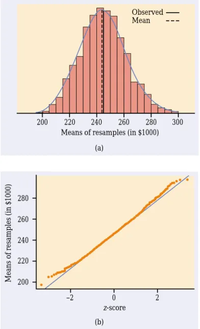
200 220 240 260 280 300 Means of resamples (in $1000)
200 220 240 260 280 –2 0 2 z-score
Means of resamples (in $1000)
(a)
(b)
Observed Mean
FIGURE 14.7 The bootstrap distribution of the 25% trimmed means of 1000 resamples from the data in Table 14.1. The boot-strap distribution is roughly normal.
distribution is approximately normal and has small bias, we can use essen-tially the same recipe with the bootstrap standard error to get a confidence interval for any parameter.
BOOTSTRAP
t
CONFIDENCE INTERVAL
Suppose that the bootstrap distribution of a statistic from an SRS of size n is approximately normal and that the bootstrap estimate of bias is small. An approximate level C confidence interval for the parameter that corresponds to this statistic by the plug-in principle is
where SEbootis the bootstrap standard error for this statistic and t∗is the critical value of the t(n−1)distribution with area C between−t∗ and t∗.
E X A M P L E 1 4 . 5 2002 Seattle real estate selling prices. Table 14.1 gives an SRS of sizeWe want to estimate the 25% trimmed mean of the population of all n = 50. The software output above shows that the trimmed mean of this sample is x25%=244 and that the bootstrap standard error of this statistic is SEboot=16.83. A
95% confidence interval for the population trimmed mean is therefore x25%±t∗SEboot=244±(2.009)(16.83)
=244±33.81
=(210.19,277.81)
Because Table D does not have entries for n−1 = 49 degrees of freedom, we used t∗=2.009, the entry for 50 degrees of freedom.
We are 95% confident that the 25% trimmed mean (the mean of the middle 50%) for the population of real estate sales in Seattle in 2002 is between $210,190 and $277,810.
Bootstrapping to compare two groups
Two-sample problems (Section 7.2) are among the most common statistical settings. In a two-sample problem, we wish to compare two populations, such as male and female college students, based on separate samples from each population. When both populations are roughly normal, the two-sample t pro-cedures compare the two population means. The bootstrap can also compare two populations, without the normality condition and without the restriction to comparison of means. The most important new idea is that bootstrap re-sampling must mimic the “separate samples” design that produced the origi-nal data.
BOOTSTRAP FOR COMPARING TWO POPULATIONS
Given independent SRSs of sizes n and m from two populations: 1. Draw a resample of size n with replacement from the first sample and a separate resample of size m from the second sample. Compute a statistic that compares the two groups, such as the difference between the two sample means.
2. Repeat this resampling process hundreds of times.
3. Construct the bootstrap distribution of the statistic. Inspect its shape, bias, and bootstrap standard error in the usual way.
E X A M P L E 1 4 . 6 customers of competing providers of telephone service (CLECs) withinWe saw in Example 14.1 that Verizon is required to perform repairs for its region. How do repair times for CLEC customers compare with times for Veri-zon’s own customers? Figure 14.8 shows density curves and normal quantile plots for the service times (in hours) of 1664 repair requests from customers of Verizon and
ILEC CLEC ILEC CLEC n = 1664 n = 23 150 100 50 0 0 50 100 150 200
Repair time (in hours)
Repair time (in hours)
(a)
–2 0 2
z-score (b)
FIGURE 14.8 Density curves and normal quantile plots of the distributions of repair times for Verizon customers and customers of a CLEC. (The density curves extend below zero because they smooth the data. There are no negative repair times.)
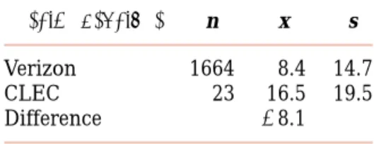
23 requests from customers of a CLEC during the same time period. The distributions are both far from normal. Here are some summary statistics:
Service provider n x¯ s
Verizon 1664 8.4 14.7
CLEC 23 16.5 19.5
Difference −8.1
The data suggest that repair times may be longer for CLEC customers. The mean repair time, for example, is almost twice as long for CLEC customers as for Verizon customers.
In the setting of Example 14.6 we want to estimate the difference of pop-ulation means,µ1−µ2. We are reluctant to use the two-sample t confidence interval because one of the samples is both small and very skewed. To com-pute the bootstrap standard error for the difference in sample means x1−x2, resample separately from the two samples. Each of our 1000 resamples con-sists of two group resamples, one of size 1664 drawn with replacement from the Verizon data and one of size 23 drawn with replacement from the CLEC data. For each combined resample, compute the statistic x1−x2. The 1000 differences form the bootstrap distribution. The bootstrap standard error is the standard deviation of the bootstrap distribution.
S-PLUS automates the proper bootstrap procedure. Here is some of the S-PLUS output:
Number of Replications: 1000
Summary Statistics:
Observed Mean Bias SE meanDiff -8.098 -8.251 -0.1534 4.052
Figure 14.9 shows that the bootstrap distribution is not close to normal. It has a short right tail and a long left tail, so that it is skewed to the left. Because
CAUTION
the bootstrap distribution is nonnormal, we can’t trust the bootstrap t confidence interval. When the sampling distribution is nonnormal, no method based on normality is safe. Fortunately, there are more general ways of using the boot-strap to get confidence intervals that can be safely applied when the bootboot-strap distribution is not normal. These methods, which we discuss in Section 14.4, are the next step in practical use of the bootstrap.
BEYOND THE BASICS
The bootstrap for a
scatterplot smoother
The bootstrap idea can be applied to quite complicated statistical methods, such as the scatterplot smoother illustrated in Chapter 2 (page 110).
0 –5 –10 –15 –20 –25 –25 –20 –15 –10 –5 0
Difference in mean repair times (in hours)
Dif
fer
ence in mean r
epair times (in hours)
(a) –2 0 2 z-score (b) Observed Mean
FIGURE 14.9 The bootstrap distribution of the differ-ence in means for the Verizon and CLEC repair time data.
E X A M P L E 1 4 . 7 state of New Jersey. We’ll analyze the first 254 drawings after the lotteryThe New Jersey Pick-It Lottery is a daily numbers game run by the was started in 1975.7 Buying a ticket entitles a player to pick a number between 000
and 999. Half of the money bet each day goes into the prize pool. (The state takes the other half.) The state picks a winning number at random, and the prize pool is shared equally among all winning tickets.
200 400 600 800 0 200 400 600 800 1000 Number Payoff Smooth Regression line
FIGURE 14.10 The first 254 winning numbers in the New Jersey Pick-It Lottery and the payoffs for each. To see patterns we use least-squares regression (line) and a scatterplot smoother (curve).
Although all numbers are equally likely to win, numbers chosen by fewer people have bigger payoffs if they win because the prize is shared among fewer tickets. Fig-ure 14.10 is a scatterplot of the first 254 winning numbers and their payoffs. What pat-terns can we see?
The straight line in Figure 14.10 is the least-squares regression line. The line shows a general trend of higher payoffs for larger winning numbers. The curve in the figure was fitted to the plot by a scatterplot smoother that follows local patterns in the data rather than being constrained to a straight line. The curve suggests that there were larger payoffs for numbers in the intervals 000 to 100, 400 to 500, 600 to 700, and 800 to 999. When people pick “random” numbers, they tend to choose numbers starting with 2, 3, 5, or 7, so these num-bers have lower payoffs. This pattern disappeared after 1976; it appears that players noticed the pattern and changed their number choices.
Are the patterns displayed by the scatterplot smoother just chance? We can use the bootstrap distribution of the smoother’s curve to get an idea of how much random variability there is in the curve. Each resample “statistic” is now a curve rather than a single number. Figure 14.11 shows the curves that result from applying the smoother to 20 resamples from the 254 data points in Figure 14.10. The original curve is the thick line. The spread of the resample curves about the original curve shows the sampling variability of the output of the scatterplot smoother.
Nearly all the bootstrap curves mimic the general pattern of the original smoother curve, showing, for example, the same low average payoffs for num-bers in the 200s and 300s. This suggests that these patterns are real, not just chance.
200 400 600 800 0 200 400 600 800 1000 Number Payoff Original smooth Bootstrap smooths
FIGURE 14.11 The curves produced by the scatterplot smoother for 20 resamples from the data displayed in Figure 14.10. The curve for the original sample is the heavy line.
SECTION 14.2
Summary
Bootstrap distributions mimic the shape, spread, and bias of sampling distributions.
The bootstrap standard error SEboot of a statistic is the standard deviation of its bootstrap distribution. It measures how much the statistic varies under random sampling.
The bootstrap estimate of the bias of a statistic is the mean of the bootstrap distribution minus the statistic for the original data. Small bias means that the bootstrap distribution is centered at the statistic of the original sample and suggests that the sampling distribution of the statistic is centered at the population parameter.
The bootstrap can estimate the sampling distribution, bias, and standard er-ror of a wide variety of statistics, such as the trimmed mean, whether or not statistical theory tells us about their sampling distributions.
If the bootstrap distribution is approximately normal and the bias is small, we can give a bootstrap t confidence interval, statistic±t∗SEboot, for the parameter. Do not use this t interval if the bootstrap distribution is not normal or shows substantial bias.
SECTION 14.2
Exercises
14.9 Return to or re-create the bootstrap distribution of the sample mean for the 72 guinea pig lifetimes in Exercise 14.6.
(a) What is the bootstrap estimate of the bias? Verify from the graphs of the bootstrap distribution that the distribution is reasonably normal (some right skew remains) and that the bias is small relative to the observed x. The bootstrap t confidence interval for the population meanµis therefore justified.
(b) Give the 95% bootstrap t confidence interval forµ.
(c) The only difference between the bootstrap t and usual one-sample t con-fidence intervals is that the bootstrap interval uses SEbootin place of the formula-based standard error s/√n. What are the values of the two stan-dard errors? Give the usual t 95% interval and compare it with your inter-val from (b).
14.10 Bootstrap distributions and quantities based on them differ randomly when
we repeat the resampling process. A key fact is that they do not differ very much if we use a large number of resamples. Figure 14.7 shows one bootstrap distribution for the trimmed mean selling price for Seattle real estate. Repeat the resampling of the data in Table 14.1 to get another bootstrap distribution for the trimmed mean.
(a) Plot the bootstrap distribution and compare it with Figure 14.7. Are the two bootstrap distributions similar?
(b) What are the values of the mean statistic, bias, and bootstrap standard error for your new bootstrap distribution? How do they compare with the previous values given on page 14-16?
(c) Find the 95% bootstrap t confidence interval based on your bootstrap dis-tribution. Compare it with the previous result in Example 14.5.
14.11 For Example 14.5 we bootstrapped the 25% trimmed mean of the 50 selling
prices in Table 14.1. Another statistic whose sampling distribution is unfa-miliar to us is the standard deviation s. Bootstrap s for these data. Discuss the shape and bias of the bootstrap distribution. Is the bootstrap t confidence interval for the population standard deviationσ justified? If it is, give a 95% confidence interval.
14.12 We will see in Section 14.3 that bootstrap methods often work poorly for the
median. To illustrate this, bootstrap the sample median of the 50 selling prices in Table 14.1. Why is the bootstrap t confidence interval not justified?
14.13 We have a formula (page 488) for the standard error of x1−x2. This formula
does not depend on normality. How does this formula-based standard error for the data of Example 14.6 compare with the bootstrap standard error?
14.14 Table 7.4 (page 491) gives the scores on a test of reading ability for two groups
of third-grade students. The treatment group used “directed reading ac-tivities” and the control group followed the same curriculum without the activities.
(a) Bootstrap the difference in meansx¯1− ¯x2and report the bootstrap stan-dard error.
(b) Inspect the bootstrap distribution. Is a bootstrap t confidence interval ap-propriate? If so, give a 95% confidence interval.
(c) Compare the bootstrap results with the two-sample t confidence interval reported on page 492.
14.15 Table 7.6 (page 512) contains the ratio of current assets to current liabilities
for random samples of healthy firms and failed firms. Find the difference in means (healthy minus failed).
(a) Bootstrap the difference in meansx¯1− ¯x2and look at the bootstrap distri-bution. Does it meet the conditions for a bootstrap t confidence interval? (b) Report the bootstrap standard error and the 95% bootstrap t confidence
interval.
(c) Compare the bootstrap results with the usual two-sample t confidence interval.
14.16 Explain the difference between the standard deviation of a sample and the
standard error of a statistic such as the sample mean.
14.17 The following data are “really normal.” They are an SRS from the standard
normal distribution N(0,1), produced by a software normal random number generator. 0.01 −0.04 −1.02 −0.13 −0.36 −0.03 −1.88 0.34 −0.00 1.21 −0.02 −1.01 0.58 0.92 −1.38 −0.47 −0.80 0.90 −1.16 0.11 0.23 2.40 0.08 −0.03 0.75 2.29 −1.11 −2.23 1.23 1.56 −0.52 0.42 −0.31 0.56 2.69 1.09 0.10 −0.92 −0.07 −1.76 0.30 −0.53 1.47 0.45 0.41 0.54 0.08 0.32 −1.35 −2.42 0.34 0.51 2.47 2.99 −1.56 1.27 1.55 0.80 −0.59 0.89 −2.36 1.27 −1.11 0.56 −1.12 0.25 0.29 0.99 0.10 0.30 0.05 1.44 −2.46 0.91 0.51 0.48 0.02 −0.54
(a) Make a histogram and normal quantile plot. Do the data appear to be “really normal”? From the histogram, does the N(0,1)distribution ap-pear to describe the data well? Why?
(b) Bootstrap the mean. Why do your bootstrap results suggest that t confi-dence intervals are appropriate?
(c) Give both the bootstrap and the formula-based standard errors for x. Give both the bootstrap and usual t 95% confidence intervals for the population meanµ.
14.18 Because the shape and bias of the bootstrap distribution approximate the
shape and bias of the sampling distribution, bootstrapping helps check whether the sampling distribution allows use of the usual t procedures. In Exercise 14.4 you bootstrapped the mean for the amount of vitamin C in a random sample of 8 lots of corn soy blend. Return to or re-create your work. (a) The sample is very small. Nonetheless, the bootstrap distribution suggests
(b) Give SEboot and the bootstrap t 95% confidence interval. How do these compare with the formula-based standard error and usual t interval given in Example 7.1 (page 453)?
14.19 Exercise 7.5 (page 473) gives data on 60 children who said how big a part they
thought luck played in solving a puzzle. The data have a discrete 1 to 10 scale. Is inference based on t distributions nonetheless justified? Explain your an-swer. If t inference is justified, compare the usual t and bootstrap t 95% con-fidence intervals.
14.20 Your company sells exercise clothing and equipment on the Internet. To
de-sign clothing, you collect data on the physical characteristics of your cus-tomers. Here are the weights in kilograms for a sample of 25 male runners. Assume these runners are a random sample of your potential male customers.
67.8 61.9 63.0 53.1 62.3 59.7 55.4 58.9 60.9
69.2 63.7 68.3 92.3 64.7 65.6 56.0 57.8 66.0
62.9 53.6 65.0 55.8 60.4 69.3 61.7
Because your products are intended for the “average male runner,” you are interested in seeing how much the subjects in your sample vary from the av-erage weight.
(a) Calculate the sample standard deviation s for these weights.
(b) We have no formula for the standard error of s. Find the bootstrap stan-dard error for s.
(c) What does the standard error indicate about how accurate the sample standard deviation is as an estimate of the population standard deviation?
(d) Would it be appropriate to give a bootstrap t interval for the population standard deviation? Why or why not?
14.21 Each year, the business magazine Forbes publishes a list of the world’s
billion-CHALLENGE aires. In 2002, the magazine found 497 billionaires. Here is the wealth, as
es-timated by Forbes and rounded to the nearest $100 million, of an SRS of 20 of these billionaires:8
8.6 1.3 5.2 1.0 2.5 1.8 2.7 2.4 1.4 3.0
5.0 1.7 1.1 5.0 2.0 1.4 2.1 1.2 1.5 1.0
You are interested in (vaguely) “the wealth of typical billionaires.” Bootstrap an appropriate statistic, inspect the bootstrap distribution, and draw conclu-sions based on this sample.
14.22 Why is the bootstrap distribution of the difference in mean Verizon and CLEC
repair times in Figure 14.9 so skewed? Let’s investigate by bootstrapping the mean of the CLEC data and comparing it with the bootstrap distribution for the mean for Verizon customers. The 23 CLEC repair times (in hours) are
26.62 8.60 0 21.15 8.33 20.28 96.32 17.97
3.42 0.07 24.38 19.88 14.33 5.45 5.40 2.68
(a) Bootstrap the mean for the CLEC data. Compare the bootstrap distribu-tion with the bootstrap distribudistribu-tion of the Verizon repair times in Fig-ure 14.3.
(b) Based on what you see in (a), what is the source of the skew in the boot-strap distribution of the difference in means x1−x2?
14.3 How Accurate Is a Bootstrap
Distribution?
∗
We said earlier that “When can I safely bootstrap?” is a somewhat subtle issue. Now we will give some insight into this issue.
We understand that a statistic will vary from sample to sample, so that in-ference about the population must take this random variation into account. The sampling distribution of a statistic displays the variation in the statistic due to selecting samples at random from the population. For example, the margin of error in a confidence interval expresses the uncertainty due to sam-pling variation. Now we have used the bootstrap distribution as a substitute for the sampling distribution. This introduces a second source of random vari-ation: resamples are chosen at random from the original sample.
SOURCES OF VARIATION AMONG BOOTSTRAP
DISTRIBUTIONS
Bootstrap distributions and conclusions based on them include two sources of random variation:
1. Choosing an original sample at random from the population. 2. Choosing bootstrap resamples at random from the original sample.
A statistic in a given setting has only one sampling distribution. It has many bootstrap distributions, formed by the two-step process just described. Bootstrap inference generates one bootstrap distribution and uses it to tell us about the sampling distribution. Can we trust such inference?
Figure 14.12 displays an example of the entire process. The population dis-tribution (top left) has two peaks and is far from normal. The histograms in the left column of the figure show five random samples from this population, each of size 50. The line in each histogram marks the mean x of that sample. These vary from sample to sample. The distribution of the x-values from all possible samples is the sampling distribution. This sampling distribution ap-pears to the right of the population distribution. It is close to normal, as we expect because of the central limit theorem.
Now draw 1000 resamples from an original sample, calculate x for each resample, and present the 1000 x’s in a histogram. This is a bootstrap distri-bution for x. The middle column in Figure 14.12 displays five bootstrap dis-tributions based on 1000 resamples from each of the five samples. The right *This section is optional.
–3 0 µ 3 6 0 µ 3 0 x x x x 3 0 3 0 3 Sample 1 0 3 0 x 3 0 x 3 Sample 2 0 x 3 0 x 3 0 x 3 Sample 3 0 x 3 0 x 3 0 x 3 Sample 4 0 x 3 0 x 3 0 x 3
Sample 5 Bootstrap distribution 6 for Sample 1 Bootstrap distribution for Sample 1 Bootstrap distribution for Sample 2 Bootstrap distribution for Sample 3 Bootstrap distribution for Sample 4 Bootstrap distribution for Sample 5 Bootstrap distribution 2 for Sample 1 Bootstrap distribution 3 for Sample 1 Bootstrap distribution 4 for Sample 1 Bootstrap distribution 5 for Sample 1 Sample mean = x– – – – – – – – – – – – – – – –
FIGURE 14.12 Five random samples (n=50) from the same population, with a bootstrap distribution for the sample mean formed by resampling from each of the five samples. At the right are five more bootstrap distributions from the first sample.
column shows the results of repeating the resampling from the first sample five more times. Compare the five bootstrap distributions in the middle col-umn to see the effect of the random choice of the original samples. Compare the six bootstrap distributions drawn from the first sample to see the effect of the random resampling. Here’s what we see:
• Each bootstrap distribution is centered close to the value of x for its origi-nal sample. That is, the bootstrap estimate of bias is small in all five cases. Of course, the five x-values vary, and not all are close to the population meanµ.
• The shape and spread of the bootstrap distributions in the middle column vary a bit, but all five resemble the sampling distribution in shape and spread. That is, the shape and spread of a bootstrap distribution do de-pend on the original sample, but the variation from sample to sample is not great.
• The six bootstrap distributions from the same sample are very similar in shape, center, and spread. That is, random resampling adds very little vari-ation to the varivari-ation due to the random choice of the original sample from the population.
Figure 14.12 reinforces facts that we have already relied on. If a bootstrap distribution is based on a moderately large sample from the population, its shape and spread don’t depend heavily on the original sample and do mimic the shape and spread of the sampling distribution. Bootstrap distributions do not have the same center as the sampling distribution; they mimic bias, not the actual center. The figure also illustrates a fact that is important for prac-tical use of the bootstrap: the bootstrap resampling process (using 1000 or more resamples) introduces very little additional variation. We can rely on a bootstrap distribution to inform us about the shape, bias, and spread of the sampling distribution.
Bootstrapping small samples
We now know that almost all of the variation among bootstrap distributions for a statistic such as the mean comes from the random selection of the orig-inal sample from the population. We also know that in general statisticians prefer large samples because small samples give more variable results. This general fact is also true for bootstrap procedures.
Figure 14.13 repeats Figure 14.12, with two important differences. The five original samples are only of size n=9, rather than the n=50 of Figure 14.12. The population distribution (top left) is normal, so that the sampling distri-bution of x is normal despite the small sample size. The bootstrap distribu-tions in the middle column show much more variation in shape and spread than those for larger samples in Figure 14.12. Notice, for example, how the skewness of the fourth sample produces a skewed bootstrap distribution. The bootstrap distributions are no longer all similar to the sampling distribution at the top of the column. We can’t trust a bootstrap distribution from a very
CAUTION
small sample to closely mimic the shape and spread of the sampling distribu-tion. Bootstrap confidence intervals will sometimes be too long or too short, or too long in one direction and too short in the other. The six bootstrap dis-tributions based on the first sample are again very similar. Because we used
–3 3 –3 3 –3 3 Bootstrap distribution for Sample 1 –3 –3 3 Bootstrap distribution 2 for Sample 1 –3 3 Bootstrap distribution 3 for Sample 1 –3 3 Bootstrap distribution 4 for Sample 1 –3 3 Bootstrap distribution 5 for Sample 1 –3 3 Bootstrap distribution 6 for Sample 1 –3 3 Bootstrap distribution for Sample 2 –3 3 Bootstrap distribution for Sample 3 –3 3 Bootstrap distribution for Sample 4 –3 3 Bootstrap distribution for Sample 5 3 Sample 1 –3 3 Sample 2 –3 3 Sample 3 –3 3 Sample 4 –3 3 Sample 5 x _ x_ x_ x _ x_ x _ x _ x _ x _ x _ x_ x _ x _ x_ x_
FIGURE 14.13 Five random samples (n=9) from the same population, with a bootstrap distribution for the sample mean formed by resampling from each of the five samples. At the right are five more bootstrap distributions from the first sample.
1000 resamples, resampling adds very little variation. There are subtle effects that can’t be seen from a few pictures, but the main conclusions are clear.
VARIATION IN BOOTSTRAP DISTRIBUTIONS
For most statistics, almost all the variation among bootstrap distribu-tions comes from the selection of the original sample from the popu-lation. You can reduce this variation by using a larger original sample. Bootstrapping does not overcome the weakness of small samples as a basis for inference. We will describe some bootstrap procedures that are usually more accurate than standard methods, but even they may not be accurate for very small samples. Use caution in any inference— including bootstrap inference—from a small sample.
The bootstrap resampling process using 1000 or more resamples in-troduces very little additional variation.
Bootstrapping a sample median
In dealing with the real estate sales prices in Example 14.4, we chose to boot-strap the 25% trimmed mean rather than the median. We did this in part be-cause the usual bootstrapping procedure doesn’t work well for the median unless the original sample is quite large. Now we will bootstrap the median in order to understand the difficulties.
Figure 14.14 follows the format of Figures 14.12 and 14.13. The popula-tion distribupopula-tion appears at top left, with the populapopula-tion median M marked. Below in the left column are five samples of size n=15 from this population, with their sample medians m marked. Bootstrap distributions for the me-dian based on resampling from each of the five samples appear in the middle column. The right column again displays five more bootstrap distributions from resampling the first sample. The six bootstrap distributions from the same sample are once again very similar to each other—resampling adds little variation—so we concentrate on the middle column in the figure.
Bootstrap distributions from the five samples differ markedly from each other and from the sampling distribution at the top of the column. Here’s why. The median of a resample of size 15 is the 8th-largest observation in the re-sample. This is always one of the 15 observations in the original sample and is usually one of the middle observations. Each bootstrap distribution therefore repeats the same few values, and these values depend on the original sample. The sampling distribution, on the other hand, contains the medians of all pos-sible samples and is not confined to a few values.
The difficulty is somewhat less when n is even, because the median is then the average of two observations. It is much less for moderately large samples, say n=100 or more. Bootstrap standard errors and confidence intervals from such samples are reasonably accurate, though the shapes of the bootstrap dis-tributions may still appear odd. You can see that the same difficulty will occur for small samples with other statistics, such as the quartiles, that are calcu-lated from just one or two observations from a sample.
–4 M 10 –4 M 10 –4 m 10 Bootstrap distribution for Sample 1 –4 m 10 Bootstrap distribution 2 for Sample 1 –4 m 10 Bootstrap distribution 3 for Sample 1 –4 m 10 Bootstrap distribution 4 for Sample 1 –4 m 10 Bootstrap distribution 5 for Sample 1 –4 m 10 Bootstrap distribution 6 for Sample 1 –4 m 10 Bootstrap distribution for Sample 2 –4 m 10 Bootstrap distribution for Sample 3 –4 m 10 Bootstrap distribution for Sample 4 –4 m 10 Bootstrap distribution for Sample 5 –4 m 10 Sample 1 –4 m 10 Sample 2 –4 m 10 Sample 3 –4 m 10 Sample 4 –4 m 10 Sample 5 Sample median = m
FIGURE 14.14 Five random samples (n=15) from the same population, with a bootstrap distribution for the sample median formed by resampling from each of the five samples. At the right are five more bootstrap distributions from the first sample.
There are more advanced variations of the bootstrap idea that improve performance for small samples and for statistics such as the median and quar-tiles. Unless you have expert advice or undertake further study, avoid
bootstrap-CAUTION
ping the median and quartiles unless your sample is rather large.
SECTION 14.3
Summary
Almost all of the variation among bootstrap distributions for a statistic is due to the selection of the original random sample from the population. Resam-pling introduces little additional variation.
Bootstrap distributions based on small samples can be quite variable. Their shape and spread reflect the characteristics of the sample and may not accu-rately estimate the shape and spread of the sampling distribution. Bootstrap inference from a small sample may therefore be unreliable.
Bootstrap inference based on samples of moderate size is unreliable for statis-tics like the median and quartiles that are calculated from just a few of the sample observations.
SECTION 14.3
Exercises
14.23 Most statistical software includes a function to generate samples from normal
distributions. Set the mean to 8.4 and the standard deviation to 14.7. You can think of all the numbers that would be produced by this function if it ran for-ever as a population that has the N(8.4,14.7)distribution. Samples produced by the function are samples from this population.
(a) What is the exact sampling distribution of the sample mean x for a sample of size n from this population?
(b) Draw an SRS of size n =10 from this population. Bootstrap the sample mean x using 1000 resamples from your sample. Give a histogram of the bootstrap distribution and the bootstrap standard error.
(c) Repeat the same process for samples of sizes n=40 and n=160. (d) Write a careful description comparing the three bootstrap distributions
and also comparing them with the exact sampling distribution. What are the effects of increasing the sample size?
14.24 The data for Example 14.1 are 1664 repair times for customers of Verizon,
the local telephone company in their area. In that example, these observations formed a sample. Now we will treat these 1664 observations as a population. The population distribution is pictured in Figures 14.1 and 14.8. It is very non-normal. The population mean isµ=8.4, and the population standard devia-tion isσ =14.7.
(a) Although we don’t know the shape of the sampling distribution of the sample mean x for a sample of size n from this population, we do know the mean and standard deviation of this distribution. What are they?
(b) Draw an SRS of size n =10 from this population. Bootstrap the sample mean x using 1000 resamples from your sample. Give a histogram of the bootstrap distribution and the bootstrap standard error.
(c) Repeat the same process for samples of sizes n=40 and n=160. (d) Write a careful description comparing the three bootstrap distributions.
What are the effects of increasing the sample size?
14.25 The populations in the two previous exercises have the same mean and
stan-dard deviation, but one is very close to normal and the other is strongly non-normal. Based on your work in these exercises, how does nonnormality of the population affect the bootstrap distribution of x? How does it affect the boot-strap standard error? Does either of these effects diminish when we start with a larger sample? Explain what you have observed based on what you know about the sampling distribution of x and the way in which bootstrap distri-butions mimic the sampling distribution.
14.4 Bootstrap Confidence Intervals
To this point, we have met just one type of inference procedure based on re-sampling, the bootstrap t confidence intervals. We can calculate a bootstrap t confidence interval for any parameter by bootstrapping the corresponding statistic. We don’t need conditions on the population or special knowledge about the sampling distribution of the statistic. The flexible and almost auto-matic nature of bootstrap t intervals is appealing—but there is a catch. These intervals work well only when the bootstrap distribution tells us that the sam-pling distribution is approximately normal and has small bias. How well must these conditions be met? What can we do if we don’t trust the bootstrap t in-terval? In this section we will see how to quickly check t confidence intervals for accuracy and learn alternative bootstrap confidence intervals that can be used more generally than the bootstrap t.
Bootstrap percentile confidence intervals
Confidence intervals are based on the sampling distribution of a statistic. If a statistic has no bias as an estimator of a parameter, its sampling distribution is centered at the true value of the parameter. We can then get a 95% con-fidence interval by marking off the central 95% of the sampling distribution. The t critical values in a t confidence interval are a shortcut to marking off the central 95%. The shortcut doesn’t work under all conditions—it depends both on lack of bias and on normality. One way to check whether t intervals (using either bootstrap or formula-based standard errors) are reasonable is to com-pare them with the central 95% of the bootstrap distribution. The 2.5% and 97.5% percentiles mark off the central 95%. The interval between the 2.5% and 97.5% percentiles of the bootstrap distribution is often used as a confi-dence interval in its own right. It is known as a bootstrap percentile conficonfi-dence interval.
BOOTSTRAP PERCENTILE CONFIDENCE INTERVALS
The interval between the 2.5% and 97.5% percentiles of the bootstrap distribution of a statistic is a 95% bootstrap percentile confidence interval for the corresponding parameter. Use this method when the bootstrap estimate of bias is small.
The conditions for safe use of bootstrap t and bootstrap percentile inter-vals are a bit vague. We recommend that you check whether these interinter-vals are reasonable by comparing them with each other. If the bias of the bootstrap distribution is small and the distribution is close to normal, the bootstrap t and percentile confidence intervals will agree closely. Percentile intervals, un-like t intervals, do not ignore skewness. Percentile intervals are therefore usu-ally more accurate, as long as the bias is small. Because we will soon meet much more accurate bootstrap intervals, our recommendation is that when
CAUTION
bootstrap t and bootstrap percentile intervals do not agree closely, neither type of interval should be used.
E X A M P L E 1 4 . 8 dence interval for the 25% trimmed mean of Seattle real estate salesIn Example 14.5 (page 14-18) we found that a 95% bootstrap t confi-prices is 210.2 to 277.8. The bootstrap distribution in Figure 14.7 shows a small bias and, though roughly normal, is a bit skewed. Is the bootstrap t confidence interval ac-curate for these data?
The S-PLUS bootstrap output includes the 2.5% and 97.5% percentiles of the bootstrap distribution. They are 213.1 and 279.4. These are the endpoints of the 95% bootstrap percentile confidence interval. This interval is quite close to the bootstrap t interval. We conclude that both intervals are reasonably accurate.
The bootstrap t interval for the trimmed mean of real estate sales in Ex-ample 14.8 is
x25%±t∗SEboot=244±33.81
We can learn something by also writing the percentile interval starting at the statistic x25%=244. In this form, it is
244.0−30.9, 244.0+35.4
Unlike the t interval, the percentile interval is not symmetric—its endpoints are different distances from the statistic. The slightly greater distance to the 97.5% percentile reflects the slight right skewness of the bootstrap distribution.
Confidence intervals for the correlation
The bootstrap allows us to find standard errors and confidence intervals for a wide variety of statistics. We have done this for the mean and the trimmed mean. We also learned how to find the bootstrap distribution for a differ-ence of means, but that distribution for the Verizon data (Example 14.6,