METHODS OF ESTIMATING THE PARAMETERS OF THE
QUASI LINDLEY DISTRIBUTION
Festus C. Opone1
Department of Mathematics, University of Benin, Benin City, Nigeria Nosakhare Ekhosuehi
Department of Mathematics, University of Benin, Benin City, Nigeria
1. INTRODUCTION
The Lindley distribution introduced by Lindley (1958) have received considerable atten-tion in developing a generalized form of the distribuatten-tion. Ghitanyet al.(2013) proposed the power Lindley distribution as an extension of the classical one-parameter Lindley distribution by considering the power transformationX =Tα1. Shankeret al.(2013)
in-troduced a two-parameter Lindley distribution which they call the Sushila distribution. Shibu and Irshad (2016) proposed the extended new generalized Lindley distribution, a variant of this distribution is the new extended generalized Lindley distribution intro-duced in Maya and Irshad (2017).
Shanker and Mishra (2013) proposed the quasi Lindley distribution (QLD) with pa-rameters(α,θ)and its probability density function is defined by
f(x,α,θ) =θ(α+xθ)e−θx
α+1 , x>0,θ >0,α >−1. (1) The QLD which is an extension of the one-parameter Lindley distribution is a two-component mixture of exponential(θ)and a special case of gamma(2,θ)distribution. Equation (1) can also be written in the form
f(x,α,θ) =p f1(x) + (1−p)f2(x), (2) where f1(x) =θe−θx and f
2(x) =θ2e−θx are the density functions of the exponential distribution(θ)and gamma distribution(2,θ)respectively andp = α+α1 is the mixing proportion.
The corresponding cumulative distribution function of the QLD is given by
F(x,α,θ) =1−(1+α+xθ)e
−θx
α+1 , x>0,θ >0,α >−1. (3) Amongst the mathematical properties of the distribution studied were; the shape of density function, cumulative distribution function, failure rate function, mean residual life function, stochastic ordering and its moments with related measures. The method of moments and maximum likelihood was used in estimation of the parameters of the dis-tribution and was applied to a real lifetime data set. It was shown that the quasi Lindley distribution can be used as an alternative model to the one-parameter Lindley distribu-tion and the popular exponential distribudistribu-tion, as it provides better fit in applicability to lifetime data. For more detail on the mathematical properties of the QLD, we refer readers to Shanker and Mishra (2013).
In spite of the mathematical properties studied, Shanker and Mishra (2013) did not address the quantile function of the distribution which can be used to generate random samples from the distribution. Although, the method of moment and maximum likeli-hood were used in estimation of the parameters of the distribution, their work fails to examine the performance and accuracy of the parameter estimates of the distribution. These pitfalls form the basis of our study.
Motivation of this paper arose from the work of Roozegar and Nadarajah (2017), which presents meaningful criticism and useful suggestions on the generalized Lindley distribution proposed by Nedjar and Zeghdoudi (2016). The remaining sections of this paper are organized as follows: Section 2 presents the quantile function of the quasi Lindley distribution. In Section 3, the method of moment and the maximum likeli-hood for parameter estimation are considered and a simulation study was conducted to examine the behaviour of the estimators of each parameter. Finally, in Section 4, we ex-amined the applicability of the QLD alongside with other related existing distributions in modeling lifetime data sets.
2. QUANTILE FUNCTION OF THE QUASILINDLEY DISTRIBUTION
Jodra (2010) derived a closed-form expression for the quantile function of probability distributions which are related to the LambertW function. This expression enables us to generate random samples from the distribution through the use of inverse transform. THEOREM1. For anyθ >0,α >−1, the quantile function of the quasi Lindley distri-bution X is defined by
x = −θ1−αθ−θ1W−1
−(1−u)(α+1) e(1+α)
, (4)
PROOF. LetF(x)be the distribution function of the QLD defined in Equation (3). For anyθ >0,α >−1 and 0< u<1, we need to setF(x) =uto obtain a system of non-linear equation which is given by
−(1+α+θx)e−θx = (u−1)(α+1). (5) Multiplying both sides of Equation (5) bye−(1+α), we obtain
−(1+α+θx)e−(θx+α+1) = −(1−u)(α+1)e−(1+α). (6) From Equation (6), we see that−(1+α+θx)is the LambertW function of the real argument−(1−u)(α+1)e−(1+α). Thus, we have
W
−(1−u)(α+1) e(1+α)
= −(1+α+θx). (7)
Moreover, for anyθ >0,α >−1 andx>0 ,it is immediate that(1+α+θx)>1 and it can also be checked that(1−u)(α+1)e−(1+α)ε(−1
e, 0)sinceuε(0, 1). Therefore, by
taking into account the properties of the negative branch of the LambertW function, Equation (7) becomes
W−1
−(1−u)(α+1) e(1+α)
= −(1+α+θx)
x = −1 θ−
α θ−
1 θW−1
−(1−u)(α+1) e(1+α)
. (8)
This completes the proof. 2
TABLE 1
Some quantiles of the QLD for selected values of the parameters.
u (θ=0.3,α=0.1) (θ=0.1,α=0.5) (θ=0.2,α=2) (θ=2,α=1)
0.01 0.2722 0.2958 0.0753 0.0272
0.02 0.4667 0.5839 0.1511 0.0505
0.03 0.6302 0.8657 0.2276 0.0715
0.04 0.7759 1.1419 0.3046 0.0911
0.05 0.9098 1.4134 0.3823 0.1094
0.06 1.0351 1.6809 0.4606 0.1268
0.07 1.1540 1.9448 0.5395 0.1435
0.08 1.2678 2.2058 0.6191 0.1597
0.09 1.3776 2.4641 0.6994 0.1753
Oluyedeet al.(2016), also suggested an explicit form of expressing the quantile func-tion of probability distribufunc-tions using numerical method. As an alternative to the in-verse transform method, random samples from probability distribution are generated by solving the system of non-linear equation defined in Equation (5) using numerical method. The quantiles in Table 1 was generated by solving the system of non-linear equation given in Equation (5).
3. PARAMETER ESTIMATION
3.1. Method of maximum likelihood (MLM)
Letx1,x2,· · ·,xnbe a random sample of sizenfrom QLD(α,θ), then the log-likelihood estimate is defined by
`(x,α,θ) =
n
X
i=1 log
θ(α+xθ)
e−θx α+1
(9)
= nlogθ−nlog(α+1) +
n
X
i=1
log(α+xθ)−nθX¯. (10)
The associated score function is defined by ∂ `
∂ θ = n θ+
n
X
i=1 x
(α+xθ)−nX¯=0, (11)
∂ `
∂ α = − n α+1+
n
X
i=1 1
(α+xθ)=0. (12)
The maximum likelihood estimators ˆθand ˆαcan be achieved using the Newton Raphson iterative method.
3.2. Method of moment (MOM)
The moment estimation is a technique for constructing an estimator of a parameter that is based on matching the sample moments with the corresponding distribution (theo-retical) moments.
Letx1,x2,· · ·,xnrepresent a random sample of sizendrawn from a probability dis-tribution for which we seek an unbiased estimator for thert hmoment. An expression
for the sample moment is given by
m0r= 1 n
n
X
r=1
Shanker and Mishra (2013) defined thert hmoment of the quasi Lindley distribution
as
µ0
r =
Γ(r+1)(α+r+1)
θr(α+1) , r=1, 2, 3, ... (14)
Takingr =1, 2, 3 and 4 in Equation (14), the first four raw moments of the QLD are obtained as
µ0 1=
1 θ
α+2
α+1
, µ02= 2 θ2
α+3
α+1
, µ03= 6 θ3
α+4
α+1
, µ04=24 θ4
α+5
α+1
.
Equating Equations (13) and (14), when r =1, an estimate for the parameterθis obtained as
ˆ θ= 1¯
X
α+2
α+1
. (15)
Similarly, to obtain an estimate for the parameterα, we divide the second moment by the square of the first moment to get an expression which is a function ofαonly.
µ0 2 µ2 1
=2(α+3)(α+1)
(α+2)2 =k. (16) Equation (16) results to a system of quadratic equation given by
(2−k)α2+4(2−k)α+ (6−4k) =0. (17) Solving the system of equations in (17), an expression for the estimate ofαis obtained as
ˆ
α=−(4−2k) +
p 4−2k
2−k , (18)
wherekis obtained by replacing the first moment(µ01)and the second moment(µ02)by m10 andm20 respectively.
3.3. Interval estimates
In this subsection, the asymptotic confidence intervals for the parameters of the QLD are presented. Under the normality condition, ˆη∼N[η,I−1(η)], i.e. the asymptotic distribution of an estimator ˆηof a parameterηis approximately normal with meanηand variance obtained by inverting the Fisher information matrix. The Fisher information matrix is given by
I(ηk) = −E
∂2`
∂ η2
=−E
∂2` (∂ θ)2
∂2` ∂ θ∂ α
∂2` ∂ α∂ θ ∂
2` (∂ α)2
, η= (θ,α)
where
∂2`
(∂ θ)2 = − n
X
i=1 x2 (α+xθ)2−
n θ2,
∂2`
∂ θ∂ α = ∂
2` ∂ α∂ θ =
n
X
i=1 x
(α+xθ)2,
∂2` (∂ α)2 =
n (α+1)2−
n
X
i=1 1
(α+xθ)2.
The approximate(1−δ)100 CIs for the parametersθandαare respectively ˆα± Zδ
2
p
var(αˆ)and ˆθ±Zδ 2
q
var(θˆ), where var(αˆ)and var(θˆ)are the variance ofα and θwhich are given by the first and second diagonal element of the variance-covariance matrixI−1(ηk)andZδ
2 is the upper( δ
2)percentile of the standard normal distribution.
3.4. Simulation study
In this subsection, we consider two methods of parameter estimation (MLM and MOM) to investigate the performance and accuracy of the parameter estimates of the QLD. The flexibility of these methods are compared through a simulation study for different parameter values as well as different sample sizes. We generated random data from the QLD using Equation (5). The Monte Carlo simulation study is repeated 1000 times for different sample sizesn=60,90,120,150 and parameter values (θ=0.35,α=0.15), (θ
=1,α=0.2) and (θ=2,α=0.3).
An algorithm for the simulation study is given by the following steps. 1. Choose the valueN(i.e. number of Monte Carlo simulation);
2. choose the valuesη0= (θ0,α0)corresponding to the parameters of the QLD(θ,α); 3. generate a sample of sizenfrom QLD;
4. compute the maximum likelihood estimates ˆη0ofη0 and the moment estimate defined in Equations (15) and (18);
5. repeat steps (3-4),N-times;
6. compute the bias=N1
N
X
i=1
(ηˆi−η0)and the mean square error (MSE)=N1 N
X
i=1 (ηˆi− η0)2.
TABLE 2
Monte Carlo simulation results forα=0.2,θ=1. n Methods Bias(α) Bias(θ) MSE(α) MSE(θ)
60 MLM 0.0338 0.0266 0.1010 0.0225
MOM 0.0527 0.0397 0.3602 0.0286
90 MLM 0.0296 0.0168 0.0481 0.0119
MOM 0.0368 0.0284 0.1206 0.0170
120 MLM 0.0256 0.0033 0.0334 0.0090
MOM 0.0271 0.0185 0.0890 0.0134
150 MLM 0.0153 0.0011 0.0291 0.0069
MOM 0.0188 0.0108 0.0574 0.0106
TABLE 3
Monte Carlo simulation results forα=0.3,θ=2. n Methods Bias(α) Bias(θ) MSE(α) MSE(θ)
60 MLM 0.0605 0.0447 0.2462 0.1003
MOM 0.0661 0.0790 0.3550 0.1151
90 MLM 0.0316 0.0258 0.0809 0.0526
MOM 0.0505 0.0450 0.1517 0.0744
120 MLM 0.0266 0.0181 0.0645 0.0409
MOM 0.0454 0.0357 0.1422 0.0646
150 MLM 0.0243 0.0058 0.0479 0.0290
TABLE 4
Monte Carlo simulation results forα=0.15,θ=0.35. n Methods Bias(α) Bias(θ) MSE(α) MSE(θ)
60 MLM 0.0467 0.0137 0.1628 0.0027
MOM 0.0625 0.0145 0.5057 0.0031
90 MLM 0.0299 0.0042 0.0552 0.0015
MOM 0.0506 0.0069 0.1114 0.0022
120 MLM 0.0263 0.0025 0.0320 0.0011
MOM 0.0461 0.0043 0.0975 0.0016
150 MLM 0.0066 0.0004 0.0231 0.0008
MOM 0.0067 0.0030 0.0501 0.0012
Evidently, as the sample sizenincreases, the values of the bias and the mean square error of the parameter estimates for both methods decreases and hence the estimation precision of the parameters increases. Although, the method of moment has a closed form expression for the parameter estimates, the method of maximum likelihood per-forms better for all sample size considered, therefore we recommend the method of max-imum likelihood in estimating the parameters of the quasi Lindley distribution.
4. DATA ANALYSIS
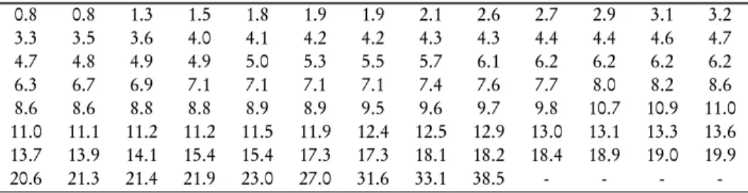
In this section, we applied the quasi Lindley distribution to a real lifetime data and com-pare its fit with the ones attained by power Lindley distribution (PLD), Sushila distribu-tion and Lindley distribudistribu-tion. Table 5 shows the waiting time (in minutes) of 100 Bank customers reported in Ghitanyet al.(2008).
TABLE 5 Waiting time data.
0.8 0.8 1.3 1.5 1.8 1.9 1.9 2.1 2.6 2.7 2.9 3.1 3.2 3.3 3.5 3.6 4.0 4.1 4.2 4.2 4.3 4.3 4.4 4.4 4.6 4.7 4.7 4.8 4.9 4.9 5.0 5.3 5.5 5.7 6.1 6.2 6.2 6.2 6.2 6.3 6.7 6.9 7.1 7.1 7.1 7.1 7.4 7.6 7.7 8.0 8.2 8.6 8.6 8.6 8.8 8.8 8.9 8.9 9.5 9.6 9.7 9.8 10.7 10.9 11.0 11.0 11.1 11.2 11.2 11.5 11.9 12.4 12.5 12.9 13.0 13.1 13.3 13.6 13.7 13.9 14.1 15.4 15.4 17.3 17.3 18.1 18.2 18.4 18.9 19.0 19.9 20.6 21.3 21.4 21.9 23.0 27.0 31.6 33.1 38.5 - - -
I−1(ηk) =
0.000299
−0.000715 −0.000715 0.0053140
and the 95% confidence intervals for the model parameters are estimated as θε(0.177291 0.245109)andαε(−0.222279 0.063478).
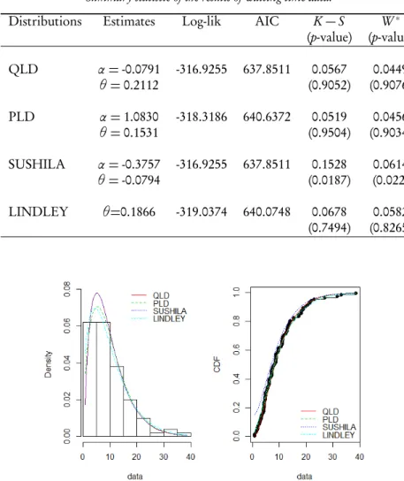
The parameter estimates, the Log-lik, Akaike information criterion (AIC), Kolmogorov-Smirnov(K−S)and the Cramér von Mises(W∗)statistic with their corresponding
p-value of the distributions for the waiting time data are shown in Table 6.
TABLE 6
Summary statistic of the results of waiting time data.
Distributions Estimates Log-lik AIC K−S W∗
(p-value) (p-value) QLD α=-0.0791 -316.9255 637.8511 0.0567 0.0449
θ=0.2112 (0.9052) (0.9076)
PLD α=1.0830 -318.3186 640.6372 0.0519 0.0456
θ=0.1531 (0.9504) (0.9034)
SUSHILA α=-0.3757 -316.9255 637.8511 0.1528 0.0614
θ=-0.0794 (0.0187) (0.022)
LINDLEY θ=0.1866 -319.0374 640.0748 0.0678 0.0582 (0.7494) (0.8265)
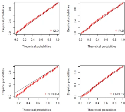
Figure 2 –Probability-Probability plot for the waiting time data.
The graphical illustration of the density and cumulative distribution fit and P-P plots of the distributions for the waiting time data is shown in Figures 1 and 2 respectively.
REFERENCES
M. GHITANY, B. ATIEH, S. NADADRAJAH(2008).Lindley distribution and its applica-tions. Mathematics and Computers in Simulation, 78, pp. 493–506.
M. GHITANY, D. AL-MUTAIRI, N. BALAKRISHNAN, I. AL-ENEZI(2013).Power Lind-ley distribution and associated inference. Computational Statistics and Data Analysis, 64, pp. 20–33.
P. JODRA (2010). Computer generation of random variables with Lindley or Pois-son–Lindley distribution via the Lambert W function. Mathematical Computations and Simulation, 81, pp. 851–859.
D. V. LINDLEY(1958).Fiducial distributions and Bayes theorem. Journal of the Royal Statistical Society, Series B, 20, no. 1, pp. 102–107.
S. NEDJAR, H. ZEGHDOUDI(2016). On gamma Lindley distribution: Properties and applications. Journal of Computational and Applied Mathematics, 298, pp. 167–174.
B.O. OLUYEDE, S. FOYA, G. WARAHENA-LIYANAGE, S. HUANG (2016). The log-logistic Weibull distribution with applications to lifetime data. Austrian Journal of Statistics, 45, pp. 43–69.
R. ROOZEGAR, S. NADARAJAH(2017).On a generalized Lindley distribution. Statistica, 77, no. 2, pp. 149–157.
R. SHANKER, A. MISHRA(2013).A quasi-Lindley distribution. African Journal of Math-ematics and Computer Science Research, 6, no. 4, pp. 64–71.
R. SHANKER, S. SHARMA, U. SHANKER, R. SHANKER(2013).Sushila distribution and its application to waiting times data. International Journal of Business Management, 3, no. 2, pp. 1–11.
D. S. SHIBU, M. R. IRSHAD(2016).Extended new generalized Lindley distribution. Sta-tistica, 76, pp. 41–56.
SUMMARY
In this paper, we review the quasi Lindley distribution and established its quantile function. A simulation study is conducted to examine the bias and mean square error of the parameter esti-mates of the distribution through the method of moment estimation and the maximum likelihood estimation. Result obtained shows that the method of maximum likelihood is a better choice of estimation method for the parameters of the quasi Lindley distribution. Finally, an applicability of the quasi Lindley disttribution to a waiting time data set suggests that the distribution demon-strates superiority over the power Lindley distribution, Sushila distribution and the classical one-parameter Lindley distribution in terms of the maximized loglikelihood, the Akaike information criterion, the Kolmogorov-Smirnov and Cramér von Mises test statistic.