Agilent Digital Modulation in Communications Systems An Introduction. Application Note 1298

Agilent

Digital Modulation in

Communications Systems

—

An Introduction

Application Note 1298

This application note introduces the concepts of digital modulation used in many communications systems today. Emphasis is placed on explaining the tradeoffs that are made to optimize efficiencies in system design.

Most communications systems fall into one of three categories: bandwidth efficient, power efficient, or cost efficient. Bandwidth efficiency describes the ability of a modulation scheme to accommodate data within a limited bandwidth. Power efficiency describes the ability of the system to reliably send information at the lowest practical power level. In most systems, there is a high priority on band-width efficiency. The parameter to be optimized depends on the demands of the particular system, as can be seen in the following two examples. For designers of digital terrestrial microwave radios, their highest priority is good bandwidth efficiency with low bit-error-rate. They have plenty of power available and are not concerned with power efficiency. They are not especially con-cerned with receiver cost or complexity because they do not have to build large numbers of them. On the other hand, designers of hand-held cellular phones put a high priority on power efficiency because these phones need to run on a battery. Cost is also a high priority because cellular phones must be low-cost to encourage more users. Accord-ingly, these systems sacrifice some bandwidth efficiency to get power and cost efficiency.

Every time one of these efficiency parameters (bandwidth, power, or cost) is increased, another one decreases, becomes more complex, or does not perform well in a poor environment. Cost is a dom-inant system priority. Low-cost radios will always be in demand. In the past, it was possible to make a radio low-cost by sacrificing power and band-width efficiency. This is no longer possible. The radio spectrum is very valuable and operators who do not use the spectrum efficiently could lose their existing licenses or lose out in the competition for new ones. These are the tradeoffs that must be considered in digital RF communications design. This application note covers

• the reasons for the move to digital modulation; • how information is modulated onto in-phase (I)

and quadrature (Q) signals;

• different types of digital modulation; • filtering techniques to conserve bandwidth; • ways of looking at digitally modulated signals; • multiplexing techniques used to share the

transmission channel;

• how a digital transmitter and receiver work; • measurements on digital RF communications

systems;

• an overview table with key specifications for the major digital communications systems; and • a glossary of terms used in digital RF

communi-cations.

These concepts form the building blocks of any communications system. If you understand the building blocks, then you will be able to under-stand how any communications system, present or future, works.

5 5 6 7 7 7 8 8 9 10 10 11 12 12 12 13 14 14 15 15 16 17 18 19 20 21 22 22 23 23 24 25 26 27 28 29 29 30

1. Why Digital Modulation?

1.1 Trading off simplicity and bandwidth 1.2 Industry trends

2. Using I/QModulation (Amplitude and Phase Control) to Convey Information

2.1 Transmitting information

2.2 Signal characteristics that can be modified 2.3 Polar display—magnitude and phase represented

together

2.4 Signal changes or modifications in polar form 2.5 I/Qformats

2.6 Iand Qin a radio transmitter 2.7 Iand Qin a radio receiver 2.8 Why use Iand Q?

3. Digital Modulation Types and Relative Efficiencies 3.1 Applications

3.1.1 Bit rate and symbol rate

3.1.2 Spectrum (bandwidth) requirements 3.1.3 Symbol clock

3.2 Phase Shift Keying (PSK) 3.3 Frequency Shift Keying 3.4 Minimum Shift Keying (MSK)

3.5 Quadrature Amplitude Modulation (QAM) 3.6 Theoretical bandwidth efficiency limits 3.7 Spectral efficiency examples in practical radios 3.8 I/Qoffset modulation

3.9 Differential modulation

3.10 Constant amplitude modulation 4. Filtering

4.1 Nyquist or raised cosine filter 4.2 Transmitter-receiver matched filters 4.3 Gaussian filter

4.4 Filter bandwidth parameter alpha 4.5 Filter bandwidth effects

4.6 Chebyshev equiripple FIR (finite impulse response) filter 4.7 Spectral efficiency versus power consumption

5. Different Ways of Looking at a Digitally Modulated Signal Time and Frequency Domain View

5.1 Power and frequency view 5.2 Constellation diagrams 5.3 Eye diagrams

32 32 32 33 33 34 34 35 35 36 37 37 37 38 38 39 39 39 40 41 41 42 43 43 44 46

6. Sharing the Channel 6.1 Multiplexing—frequency 6.2 Multiplexing—time 6.3 Multiplexing—code 6.4 Multiplexing—geography 6.5 Combining multiplexing modes 6.6 Penetration versus efficiency

7. How Digital Transmitters and Receivers Work 7.1 A digital communications transmitter

7.2 A digital communications receiver

8. Measurements on Digital RF Communications Systems 8.1 Power measurements

8.1.1 Adjacent Channel Power 8.2 Frequency measurements

8.2.1 Occupied bandwidth 8.3 Timing measurements 8.4 Modulation accuracy

8.5 Understanding Error Vector Magnitude (EVM) 8.6 Troubleshooting with error vector measurements 8.7 Magnitude versus phase error

8.8 I/Qphase error versus time 8.9 Error Vector Magnitude versus time 8.10 Error spectrum (EVM versus frequency) 9. Summary

10. Overview of Communications Systems 11. Glossary of Terms

The move to digital modulation provides more information capacity, compatibility with digital data services, higher data security, better quality communications, and quicker system availability. Developers of communications systems face these constraints:

• available bandwidth • permissible power

• inherent noise level of the system

The RF spectrum must be shared, yet every day there are more users for that spectrum as demand for communications services increases. Digital modulation schemes have greater capacity to con-vey large amounts of information than analog mod-ulation schemes.

1.1 Trading off simplicity and bandwidth

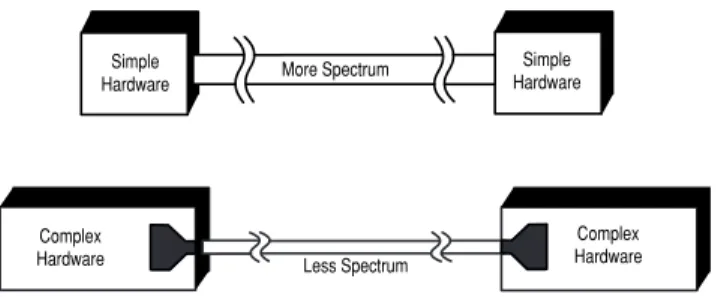
There is a fundamental tradeoff in communication systems. Simple hardware can be used in transmit-ters and receivers to communicate information. However, this uses a lot of spectrum which limits the number of users. Alternatively, more complex transmitters and receivers can be used to transmit the same information over less bandwidth. The transition to more and more spectrally efficient transmission techniques requires more and more complex hardware. Complex hardware is difficult to design, test, and build. This tradeoff exists whether communication is over air or wire, analog or digital.

Figure 1. The Fundamental Tradeoff Complex

Hardware _{Less Spectrum}

Simple Hardware Simple

Hardware

Complex Hardware More Spectrum

1.2 Industry trends

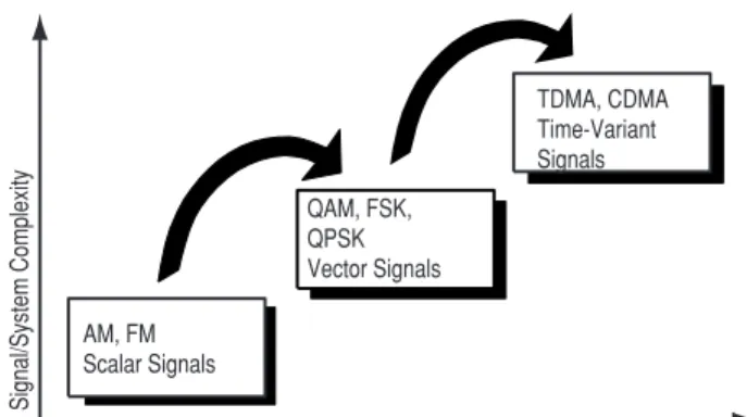
Over the past few years a major transition has occurred from simple analog Amplitude Mod-ulation (AM) and Frequency/Phase ModMod-ulation (FM/PM) to new digital modulation techniques. Examples of digital modulation include

• QPSK (Quadrature Phase Shift Keying) • FSK (Frequency Shift Keying)

• MSK (Minimum Shift Keying)

• QAM (Quadrature Amplitude Modulation) Another layer of complexity in many new systems is multiplexing. Two principal types of multiplex-ing (or “multiple access”) are TDMA (Time Division Multiple Access) and CDMA (Code Division

Multiple Access). These are two different ways to add diversity to signals allowing different signals to be separated from one another.

QAM, FSK, QPSK Vector Signals AM, FM

Scalar Signals

TDMA, CDMA Time-Variant Signals

Required Measurement Capability

Signal/System Complexity

2.1 Transmitting information

To transmit a signal over the air, there are three main steps:

1. A pure carrier is generated at the transmitter. 2. The carrier is modulated with the information

to be transmitted. Any reliably detectable change in signal characteristics can carry information.

3. At the receiver the signal modifications or changes are detected and demodulated.

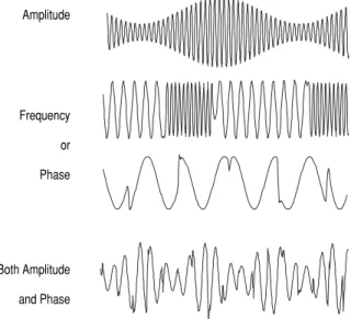
2.2 Signal characteristics that can be modified

There are only three characteristics of a signal that can be changed over time: amplitude, phase, or fre-quency. However, phase and frequency are just dif-ferent ways to view or measure the same signal change.

In AM, the amplitude of a high-frequency carrier signal is varied in proportion to the instantaneous amplitude of the modulating message signal. Frequency Modulation (FM) is the most popular analog modulation technique used in mobile com-munications systems. In FM, the amplitude of the modulating carrier is kept constant while its fre-quency is varied by the modulating message signal. Amplitude and phase can be modulated simultane-ously and separately, but this is difficult to gener-ate, and especially difficult to detect. Instead, in practical systems the signal is separated into another set of independent components: I (In-phase) and Q(Quadrature). These components are orthogonal and do not interfere with each other.

Modify a Signal "Modulate"

Detect the Modifications "Demodulate"

Any reliably detectable change in signal characteristics can carry information

Amplitude

Frequency or Phase

Both Amplitude and Phase Figure 3. Transmitting Information (Analog or Digital)

Figure 4. Signal Characteristics to Modify

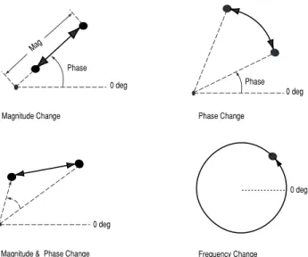
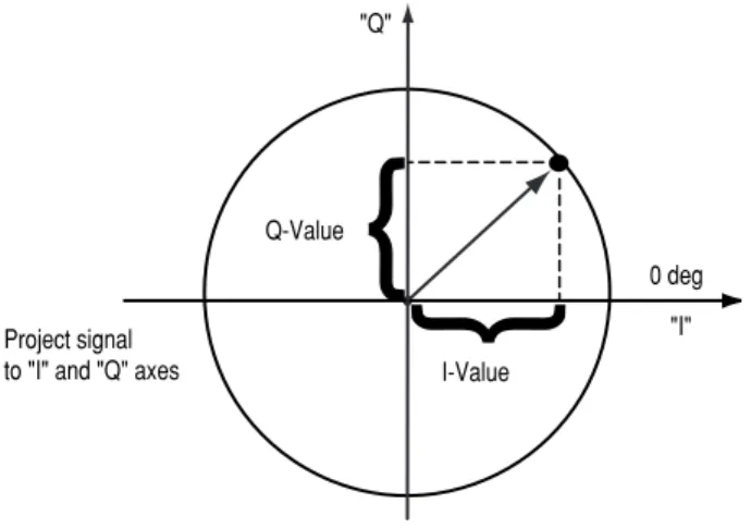
2.3 Polar display—magnitude and phase

repre-sented together

A simple way to view amplitude and phase is with the polar diagram. The carrier becomes a frequency and phase reference and the signal is interpreted relative to the carrier. The signal can be expressed in polar form as a magnitude and a phase. The phase is relative to a reference signal, the carrier in most communication systems. The magnitude is either an absolute or relative value. Both are used in digital communication systems. Polar diagrams are the basis of many displays used in digital com-munications, although it is common to describe the signal vector by its rectangular coordinates of I

(In-phase) and Q(Quadrature).

2.4 Signal changes or modifications in

polar form

Figure 6 shows different forms of modulation in polar form. Magnitude is represented as the dis-tance from the center and phase is represented as the angle.

Amplitude modulation (AM) changes only the magnitude of the signal. Phase modulation (PM) changes only the phase of the signal. Amplitude and phase modulation can be used together. Frequency modulation (FM) looks similar to phase modulation, though frequency is the controlled parameter, rather than relative phase.

Phase Mag

0 deg

Figure 5. Polar Display—Magnitude and Phase Represented Together

Phase

Mag

0 deg

Magnitude Change

Phase 0 deg

Phase Change

Frequency Change Magnitude & Phase Change

0 deg

0 deg

One example of the difficulties in RF design can be illustrated with simple amplitude modulation. Generating AM with no associated angular modula-tion should result in a straight line on a polar display. This line should run from the origin to some peak radius or amplitude value. In practice, however, the line is not straight. The amplitude modulation itself often can cause a small amount of unwanted phase modulation. The result is a curved line. It could also be a loop if there is any hysteresis in the system transfer function. Some amount of this distortion is inevitable in any sys-tem where modulation causes amplitude changes.

Therefore, the degree of effective amplitude modu-lation in a system will affect some distortion parameters.

2.5

I/Q

formats

In digital communications, modulation is often expressed in terms of Iand Q. This is a rectangular representation of the polar diagram. On a polar diagram, the Iaxis lies on the zero degree phase reference, and the Qaxis is rotated by 90 degrees. The signal vector’s projection onto the Iaxis is its “I” component and the projection onto the Qaxis is its “Q” component.

{

{

0 deg

"I" "Q"

Q-Value

I-Value Project signal

to "I" and "Q" axes

Polar to Rectangular Conversion

2.6

I

and

Q

in a radio transmitter

I/Qdiagrams are particularly useful because they mirror the way most digital communications sig-nals are created using an I/Qmodulator. In the transmitter, Iand Qsignals are mixed with the same local oscillator (LO). A 90 degree phase shifter is placed in one of the LO paths. Signals that are separated by 90 degrees are also known as being orthogonal to each other or in quadrature. Signals that are in quadrature do not interfere with each other. They are two independent compo-nents of the signal. When recombined, they are summed to a composite output signal. There are two independent signals in Iand Qthat can be sent and received with simple circuits. This simpli-fies the design of digital radios. The main advan-tage of I/Qmodulation is the symmetric ease of combining independent signal components into a single composite signal and later splitting such a composite signal into its independent component parts.

2.7

I

and

Q

in a radio receiver

The composite signal with magnitude and phase (or Iand Q) information arrives at the receiver input. The input signal is mixed with the local oscillator signal at the carrier frequency in two forms. One is at an arbitrary zero phase. The other has a 90 degree phase shift. The composite input signal (in terms of magnitude and phase) is thus broken into an in-phase, I, and a quadrature, Q, component. These two components of the signal are independent and orthogonal. One can be changed without affecting the other. Normally, information cannot be plotted in a polar format and reinterpreted as rectangular values without doing a polar-to-rectangular conversion. This con-version is exactly what is done by the in-phase and quadrature mixing processes in a digital radio. A local oscillator, phase shifter, and two mixers can perform the conversion accurately and efficiently.

90 deg Phase Shift

Local Osc. (Carrier Freq.) Q

I

Composite Output Signal

Σ

Local Osc. (Carrier Freq.)

Quadrature Component

In-Phase Component Composite

Input Signal

90 deg Phase Shift

2.8 Why use

I

and

Q

?

Digital modulation is easy to accomplish with I/Q

modulators. Most digital modulation maps the data to a number of discrete points on the I/Qplane. These are known as constellation points. As the sig-nal moves from one point to another, simultaneous amplitude and phase modulation usually results. To accomplish this with an amplitude modulator and a phase modulator is difficult and complex. It is also impossible with a conventional phase modu-lator. The signal may, in principle, circle the origin in one direction forever, necessitating infinite phase shifting capability. Alternatively, simultaneous AM and Phase Modulation is easy with an I/Qmodulator. The Iand Qcontrol signals are bounded, but infi-nite phase wrap is possible by properly phasing the Iand Qsignals.

This section covers the main digital modulation formats, their main applications, relative spectral efficiencies, and some variations of the main modulation types as used in practical systems. Fortunately, there are a limited number of modula-tion types which form the building blocks of any system.

3.1 Applications

The table below covers the applications for differ-ent modulation formats in both wireless communi-cations and video.

Although this note focuses on wireless communica-tions, video applications have also been included in the table for completeness and because of their similarity to other wireless communications.

3.1.1 Bit rate and symbol rate

To understand and compare different modulation format efficiencies, it is important to first under-stand the difference between bit rate and symbol rate. The signal bandwidth for the communications channel needed depends on the symbol rate, not on the bit rate.

Symbol rate =

Modulation format Application

MSK, GMSK GSM, CDPD

BPSK Deep space telemetry, cable modems

QPSK, π/4DQPSK Satellite, CDMA, NADC, TETRA, PHS, PDC, LMDS, DVB-S, cable (return

path), cable modems, TFTS

OQPSK CDMA, satellite

FSK, GFSK DECT, paging, RAM mobile data, AMPS, CT2, ERMES, land mobile, public safety

8, 16 VSB North American digital TV (ATV), broadcast, cable

8PSK Satellite, aircraft, telemetry pilots for monitoring broadband video systems 16 QAM Microwave digital radio, modems, DVB-C, DVB-T

32 QAM Terrestrial microwave, DVB-T

64 QAM DVB-C, modems, broadband set top boxes, MMDS 256 QAM Modems, DVB-C (Europe), Digital Video (US)

bit rate

the number of bits transmitted with each symbol

3. Digital Modulation Types and Relative Efficiencies

Bit rate is the frequency of a system bit stream. Take, for example, a radio with an 8 bit sampler, sampling at 10 kHz for voice. The bit rate, the basic bit stream rate in the radio, would be eight bits multiplied by 10K samples per second, or 80 Kbits per second. (For the moment we will ignore the extra bits required for synchronization, error correction, etc.)

Figure 10 is an example of a state diagram of a Quadrature Phase Shift Keying (QPSK) signal. The states can be mapped to zeros and ones. This is a common mapping, but it is not the only one. Any mapping can be used.

The symbol rate is the bit rate divided by the num-ber of bits that can be transmitted with each sym-bol. If one bit is transmitted per symbol, as with BPSK, then the symbol rate would be the same as the bit rate of 80 Kbits per second. If two bits are transmitted per symbol, as in QPSK, then the sym-bol rate would be half of the bit rate or 40 Kbits

per second. Symbol rate is sometimes called baud rate. Note that baud rate is not the same as bit rate. These terms are often confused. If more bits can be sent with each symbol, then the same amount of data can be sent in a narrower spec-trum. This is why modulation formats that are more complex and use a higher number of states can send the same information over a narrower piece of the RF spectrum.

3.1.2 Spectrum (bandwidth) requirements

An example of how symbol rate influences spec-trum requirements can be seen in eight-state Phase Shift Keying (8PSK). It is a variation of PSK. There are eight possible states that the signal can transi-tion to at any time. The phase of the signal can take any of eight values at any symbol time. Since 23_{= 8, there are three bits per symbol. This means}

the symbol rate is one third of the bit rate. This is relatively easy to decode.

01 00

10 11

QPSK Two Bits Per Symbol

QPSK State Diagram

BPSK One Bit Per Symbol Symbol Rate = Bit Rate

8PSK Three Bits Per Symbol Symbol Rate = 1/3 Bit Rate

3.1.3 Symbol Clock

The symbol clock represents the frequency and exact timing of the transmission of the individual symbols. At the symbol clock transitions, the trans-mitted carrier is at the correct I/Q(or magnitude/ phase) value to represent a specific symbol (a specific point in the constellation).

3.2 Phase Shift Keying

One of the simplest forms of digital modulation is binary or Bi-Phase Shift Keying (BPSK). One appli-cation where this is used is for deep space teleme-try. The phase of a constant amplitude carrier sig-nal moves between zero and 180 degrees. On an I

and Qdiagram, the Istate has two different values. There are two possible locations in the state dia-gram, so a binary one or zero can be sent. The symbol rate is one bit per symbol.

A more common type of phase modulation is Quadrature Phase Shift Keying (QPSK). It is used extensively in applications including CDMA (Code Division Multiple Access) cellular service, wireless local loop, Iridium (a voice/data satellite system) and DVB-S (Digital Video Broadcasting — Satellite). Quadrature means that the signal shifts between phase states which are separated by 90 degrees. The signal shifts in increments of 90 degrees from 45 to 135, –45, or –135 degrees. These points are chosen as they can be easily implemented using an

I/Qmodulator. Only two Ivalues and two Qvalues are needed and this gives two bits per symbol. There are four states because 22_{= 4. It is therefore}

a more bandwidth-efficient type of modulation than BPSK, potentially twice as efficient.

BPSK One Bit Per Symbol

QPSK Two Bits Per Symbol

3.3 Frequency Shift Keying

Frequency modulation and phase modulation are closely related. A static frequency shift of +1 Hz means that the phase is constantly advancing at the rate of 360 degrees per second (2 πrad/sec), relative to the phase of the unshifted signal. FSK (Frequency Shift Keying) is used in many applications including cordless and paging sys-tems. Some of the cordless systems include DECT (Digital Enhanced Cordless Telephone) and CT2 (Cordless Telephone 2).

In FSK, the frequency of the carrier is changed as a function of the modulating signal (data) being transmitted. Amplitude remains unchanged. In binary FSK (BFSK or 2FSK), a “1” is represented by one frequency and a “0” is represented by another frequency.

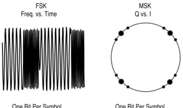
3.4 Minimum Shift Keying

Since a frequency shift produces an advancing or retarding phase, frequency shifts can be detected by sampling phase at each symbol period. Phase shifts of (2N + 1) π/2radians are easily detected with an I/Qdemodulator. At even numbered sym-bols, the polarity of the Ichannel conveys the transmitted data, while at odd numbered symbols

the polarity of the Qchannel conveys the data. This orthogonality between Iand Qsimplifies detection algorithms and hence reduces power con-sumption in a mobile receiver. The minimum fre-quency shift which yields orthogonality of Iand Q

is that which results in a phase shift of ±π/2 radi-ans per symbol (90 degrees per symbol). FSK with this deviation is called MSK (Minimum Shift Keying). The deviation must be accurate in order to generate repeatable 90 degree phase shifts. MSK is used in the GSM (Global System for Mobile

Communications) cellular standard. A phase shift of +90 degrees represents a data bit equal to “1,” while –90 degrees represents a “0.” The peak-to-peak frequency shift of an MSK signal is equal to one-half of the bit rate.

FSK and MSK produce constant envelope carrier signals, which have no amplitude variations. This is a desirable characteristic for improving the power efficiency of transmitters. Amplitude varia-tions can exercise nonlinearities in an amplifier’s amplitude-transfer function, generating spectral regrowth, a component of adjacent channel power. Therefore, more efficient amplifiers (which tend to be less linear) can be used with constant-envelope signals, reducing power consumption.

MSK Q vs. I FSK

Freq. vs. Time

One Bit Per Symbol One Bit Per Symbol

MSK has a narrower spectrum than wider devia-tion forms of FSK. The width of the spectrum is also influenced by the waveforms causing the fre-quency shift. If those waveforms have fast transi-tions or a high slew rate, then the spectrum of the transmitter will be broad. In practice, the waveforms are filtered with a Gaussian filter, resulting in a narrow spectrum. In addition, the Gaussian filter has no time-domain overshoot, which would broaden the spectrum by increasing the peak deviation. MSK with a Gaussian filter is termed GMSK (Gaussian MSK).

3.5 Quadrature Amplitude Modulation

Another member of the digital modulation family is Quadrature Amplitude Modulation (QAM). QAM is used in applications including microwave digital radio, DVB-C (Digital Video Broadcasting—Cable), and modems.

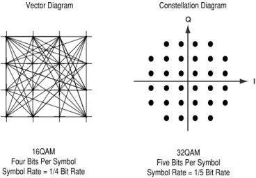
In 16-state Quadrature Amplitude Modulation (16QAM), there are four Ivalues and four Qvalues. This results in a total of 16 possible states for the signal. It can transition from any state to any other state at every symbol time. Since 16 = 24_{, four bits}

per symbol can be sent. This consists of two bits for Iand two bits for Q. The symbol rate is one fourth of the bit rate. So this modulation format

produces a more spectrally efficient transmission. It is more efficient than BPSK, QPSK, or 8PSK. Note that QPSK is the same as 4QAM.

Another variation is 32QAM. In this case there are six Ivalues and six Qvalues resulting in a total of 36 possible states (6x6=36). This is too many states for a power of two (the closest power of two is 32). So the four corner symbol states, which take the most power to transmit, are omitted. This reduces the amount of peak power the transmitter has to generate. Since 25_{= 32, there are five bits per}

sym-bol and the symsym-bol rate is one fifth of the bit rate. The current practical limits are approximately 256QAM, though work is underway to extend the limits to 512 or 1024 QAM. A 256QAM system uses 16 I-values and 16 Q-values, giving 256 possible states. Since 28_{= 256, each symbol can represent}

eight bits. A 256QAM signal that can send eight bits per symbol is very spectrally efficient. However, the symbols are very close together and are thus more subject to errors due to noise and distortion. Such a signal may have to be transmit-ted with extra power (to effectively spread the symbols out more) and this reduces power efficiency as compared to simpler schemes.

16QAM Four Bits Per Symbol Symbol Rate = 1/4 Bit Rate

I Q

32QAM Five Bits Per Symbol Symbol Rate = 1/5 Bit Rate

Vector Diagram Constellation Diagram

Compare the bandwidth efficiency when using 256QAM versus BPSK modulation in the radio example in section 3.1.1 (which uses an eight-bit sampler sampling at 10 kHz for voice). BPSK uses 80 Ksymbols-per-second sending 1 bit per symbol. A system using 256QAM sends eight bits per sym-bol so the symsym-bol rate would be 10 Ksymsym-bols per second. A 256QAM system enables the same amount of information to be sent as BPSK using only one eighth of the bandwidth. It is eight times more bandwidth efficient. However, there is a tradeoff. The radio becomes more complex and is more susceptible to errors caused by noise and dis-tortion. Error rates of higher-order QAM systems such as this degrade more rapidly than QPSK as noise or interference is introduced. A measure of this degradation would be a higher Bit Error Rate (BER).

In any digital modulation system, if the input sig-nal is distorted or severely attenuated the receiver will eventually lose symbol lock completely. If the receiver can no longer recover the symbol clock, it cannot demodulate the signal or recover any infor-mation. With less degradation, the symbol clock can be recovered, but it is noisy, and the symbol locations themselves are noisy. In some cases, a symbol will fall far enough away from its intended position that it will cross over to an adjacent posi-tion. The Iand Qlevel detectors used in the demodulator would misinterpret such a symbol as being in the wrong location, causing bit errors. QPSK is not as efficient, but the states are much

farther apart and the system can tolerate a lot more noise before suffering symbol errors. QPSK has no intermediate states between the four corner-symbol locations, so there is less opportunity for the demodulator to misinterpret symbols. QPSK requires less transmitter power than QAM to achieve the same bit error rate.

3.6 Theoretical bandwidth efficiency limits

Bandwidth efficiency describes how efficiently the allocated bandwidth is utilized or the ability of a modulation scheme to accommodate data, within a limited bandwidth. The table below shows the theoretical bandwidth efficiency limits for the main modulation types. Note that these figures cannot actually be achieved in practical radios since they require perfect modulators, demodula-tors, filter, and transmission paths.

If the radio had a perfect (rectangular in the fre-quency domain) filter, then the occupied band-width could be made equal to the symbol rate. Techniques for maximizing spectral efficiency include the following:

• Relate the data rate to the frequency shift (as in GSM).

• Use premodulation filtering to reduce the occupied bandwidth. Raised cosine filters, as used in NADC, PDC, and PHS, give the best spectral efficiency.

• Restrict the types of transitions.

Modulation Theoretical bandwidth

format efficiency limits

MSK 1 bit/second/Hz

BPSK 1 bit/second/Hz

QPSK 2 bits/second/Hz

8PSK 3 bits/second/Hz

16 QAM 4 bits/second/Hz

32 QAM 5 bits/second/Hz

64 QAM 6 bits/second/Hz

Effects of going through the origin

Take, for example, a QPSK signal where the normalized value changes from 1, 1 to –1, –1. When changing simulta-neously from I and Q values of +1 to I and Q values of –1, the signal trajectory goes through the origin (the I/Q value of 0,0). The origin represents 0 carrier magnitude. A value of 0 magnitude indicates that the carrier amplitude is 0 for a moment.

Not all transitions in QPSK result in a trajectory that goes through the origin. If I changes value but Q does not (or vice-versa) the carrier amplitude changes a little, but it does not go through zero. Therefore some symbol transi-tions will result in a small amplitude variation, while others will result in a very large amplitude variation. The clock-recovery circuit in the receiver must deal with this ampli-tude variation uncertainty if it uses ampliampli-tude variations to align the receiver clock with the transmitter clock. Spectral regrowth does not automatically result from these trajectories that pass through or near the origin. If the amplifier and associated circuits are perfectly linear, the spectrum (spectral occupancy or occupied bandwidth) will be unchanged. The problem lies in nonlinearities in the circuits.

A signal which changes amplitude over a very large range will exercise these nonlinearities to the fullest extent. These nonlinearities will cause distortion products. In con-tinuously modulated systems they will cause “spectral regrowth” or wider modulation sidebands (a phenomenon related to intermodulation distortion). Another term which is sometimes used in this context is “spectral splatter.” However this is a term that is more correctly used in asso-ciation with the increase in the bandwidth of a signal caused by pulsing on and off.

3.7 Spectral efficiency examples in

practical radios

The following examples indicate spectral efficien-cies that are achieved in some practical radio systems.

The TDMA version of the North American Digital Cellular (NADC) system, achieves a 48 Kbits-per-second data rate over a 30 kHz bandwidth or 1.6 bits per second per Hz. It is a π/4 DQPSK based system and transmits two bits per symbol. The theoretical efficiency would be two bits per second per Hz and in practice it is 1.6 bits per second per Hz.

Another example is a microwave digital radio using 16QAM. This kind of signal is more susceptible to noise and distortion than something simpler such as QPSK. This type of signal is usually sent over a direct line-of-sight microwave link or over a wire where there is very little noise and interference. In this microwave-digital-radio example the bit rate is 140 Mbits per second over a very wide bandwidth of 52.5 MHz. The spectral efficiency is 2.7 bits per second per Hz. To implement this, it takes a very clear line-of-sight transmission path and a precise and optimized high-power transceiver.

Digital modulation types—variations

The modulation types outlined in sections 3.2 to 3.4 form the building blocks for many systems. There are three main variations on these basic building blocks that are used in communications systems: I/Qoffset modulation, differential modula-tion, and constant envelope modulation.

3.8

I/Q

offset modulation

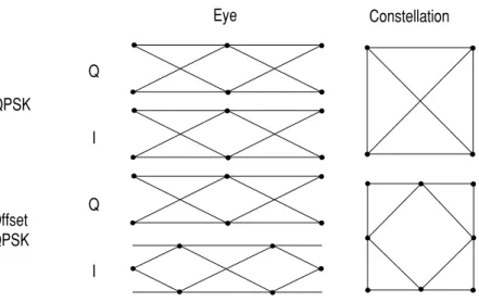
The first variation is offset modulation. One exam-ple of this is Offset QPSK (OQPSK). This is used in the cellular CDMA (Code Division Multiple Access) system for the reverse (mobile to base) link. In QPSK, the Iand Qbit streams are switched at the same time. The symbol clocks, or the Iand Q

digital signal clocks, are synchronized. In Offset

QPSK (OQPSK), the Iand Qbit streams are offset in their relative alignment by one bit period (one half of a symbol period). This is shown in the dia-gram. Since the transitions of Iand Qare offset, at any given time only one of the two bit streams can change values. This creates a dramatically different constellation, even though there are still just two

I/Qvalues. This has power efficiency advantages. In OQPSK the signal trajectories are modified by the symbol clock offset so that the carrier ampli-tude does not go through or near zero (the center of the constellation). The spectral efficiency is the same with two Istates and two Qstates. The reduced amplitude variations (perhaps 3 dB for OQPSK, versus 30 to 40 dB for QPSK) allow a more power-efficient, less linear RF power amplifier to be used.

QPSK

Offset QPSK

Q

I

Q

I

Eye Constellation

3.9 Differential modulation

The second variation is differential modulation as used in differential QPSK (DQPSK) and differential 16QAM (D16QAM). Differential means that the information is not carried by the absolute state, it is carried by the transition between states. In some cases there are also restrictions on allowable tran-sitions. This occurs in π/4DQPSK where the carrier trajectory does not go through the origin. A DQPSK transmission system can transition from any sym-bol position to any other symsym-bol position. The π/4 DQPSK modulation format is widely used in many applications including

• cellular

–NADC- IS-54 (North American digital cellular) –PDC (Pacific Digital Cellular)

• cordless

–PHS (personal handyphone system) • trunked radio

–TETRA (Trans European Trunked Radio) The π/4DQPSK modulation format uses two QPSK constellations offset by 45 degrees (π/4radians). Transitions must occur from one constellation to the other. This guarantees that there is always a change in phase at each symbol, making clock recovery easier. The data is encoded in the magni-tude and direction of the phase shift, not in the absolute position on the constellation. One advan-tage of π/4DQPSK is that the signal trajectory does not pass through the origin, thus simplifying trans-mitter design. Another is that π/4DQPSK, with root raised cosine filtering, has better spectral efficiency than GMSK, the other common cellular modulation type.

QPSK π_{/4 DQPSK}

Both formats are 2 bits/symbol

3.10 Constant amplitude modulation

The third variation is constant-envelope modula-tion. GSM uses a variation of constant amplitude modulation format called 0.3 GMSK (Gaussian Minimum Shift Keying).

In constant-envelope modulation the amplitude of the carrier is constant, regardless of the variation in the modulating signal. It is a power-efficient scheme that allows efficient class-C amplifiers to be used without introducing degradation in the spectral occupancy of the transmitted signal. However, constant-envelope modulation techniques occupy a larger bandwidth than schemes which are linear. In linear schemes, the amplitude of the transmitted signal varies with the modulating digi-tal signal as in BPSK or QPSK. In systems where

bandwidth efficiency is more important than power efficiency, constant envelope modulation is not as well suited.

MSK (covered in section 3.4) is a special type of FSK where the peak-to-peak frequency deviation is equal to half the bit rate.

GMSK is a derivative of MSK where the bandwidth required is further reduced by passing the modu-lating waveform through a Gaussian filter. The Gaussian filter minimizes the instantaneous fre-quency variations over time. GMSK is a spectrally efficient modulation scheme and is particularly useful in mobile radio systems. It has a constant envelope, spectral efficiency, good BER perform-ance, and is self-synchronizing.

MSK (GSM)

Amplitude (Envelope) Varies From Zero to Nominal Value

QPSK

Amplitude (Envelope) Does Not Vary At All

Filtering allows the transmitted bandwidth to be significantly reduced without losing the content of the digital data. This improves the spectral effi-ciency of the signal.

There are many different varieties of filtering. The most common are

• raised cosine

• square-root raised cosine • Gaussian filters

Any fast transition in a signal, whether it be ampli-tude, phase, or frequency, will require a wide occu-pied bandwidth. Any technique that helps to slow down these transitions will narrow the occupied bandwidth. Filtering serves to smooth these transi-tions (in Iand Q). Filtering reduces interference because it reduces the tendency of one signal or one transmitter to interfere with another in a Frequency-Division-Multiple-Access (FDMA) system. On the receiver end, reduced bandwidth improves sensitivity because more noise and interference are rejected.

Some tradeoffs must be made. One is that some types of filtering cause the trajectory of the signal (the path of transitions between the states) to overshoot in many cases. This overshoot can occur in certain types of filters such as Nyquist. This

overshoot path represents carrier power and phase. For the carrier to take on these values it requires more output power from the transmitter ampli-fiers. It requires more power than would be neces-sary to transmit the actual symbol itself. Carrier power cannot be clipped or limited (to reduce or eliminate the overshoot) without causing the spec-trum to spread out again. Since narrowing the spectral occupancy was the reason the filtering was inserted in the first place, it becomes a very fine balancing act.

Other tradeoffs are that filtering makes the radios more complex and can make them larger, especially if performed in an analog fashion. Filtering can also create Inter-Symbol Interference (ISI). This occurs when the signal is filtered enough so that the symbols blur together and each symbol affects those around it. This is determined by the time-domain response or impulse response of the filter.

4.1 Nyquist or raised cosine filter

Figure 18 shows the impulse or time-domain response of a raised cosine filter, one class of Nyquist filter. Nyquist filters have the property that their impulse response rings at the symbol rate. The filter is chosen to ring, or have the impulse response of the filter cross through zero, at the symbol clock frequency.

0 0.5 1

-10 _{-5 0 5 10}

h i

t i One symbol

Figure 18. Nyquit or Raised Cosine Filter

The time response of the filter goes through zero with a period that exactly corresponds to the sym-bol spacing. Adjacent symsym-bols do not interfere with each other at the symbol times because the response equals zero at all symbol times except the center (desired) one. Nyquist filters heavily filter the signal without blurring the symbols together at the symbol times. This is important for transmit-ting information without errors caused by Inter-Symbol Interference. Note that Inter-Inter-Symbol Interference does exist at all times except the sym-bol (decision) times. Usually the filter is split, half being in the transmit path and half in the receiver path. In this case root Nyquist filters (commonly called root raised cosine) are used in each part, so that their combined response is that of a Nyquist filter.

4.2 Transmitter-receiver matched filters

Sometimes filtering is desired at both the trans-mitter and receiver. Filtering in the transtrans-mitter reduces the adjacent-channel-power radiation of the transmitter, and thus its potential for interfer-ing with other transmitters.

Filtering at the receiver reduces the effects of broadband noise and also interference from other transmitters in nearby channels.

To get zero Inter-Symbol Interference (ISI), both filters are designed until the combined result of the filters and the rest of the system is a full Nyquist filter. Potential differences can cause problems in manufacturing because the transmitter and receiver are often manufactured by different companies. The receiver may be a small hand-held model and the transmitter may be a large cellular base sta-tion. If the design is performed correctly the results are the best data rate, the most efficient radio, and reduced effects of interference and noise. This is why root-Nyquist filters are used in receivers and transmitters as √Nyquist x√Nyquist = Nyquist. Matched filters are not used in Gaussian filtering.

4.3 Gaussian filter

In contrast, a GSM signal will have a small blurring of symbols on each of the four states because the Gaussian filter used in GSM does not have zero Inter-Symbol Interference. The phase states vary somewhat causing a blurring of the symbols, as shown in Figure 17. Wireless system architects must decide just how much of the Inter-Symbol Interference can be tolerated in a system and com-bine that with noise and interference.

Actual Data

Root Raised Cosine Filter

DAC

Detected Bits Root Raised

Cosine Filter

Transmitter

Receiver

Demodulator Modulator

Gaussian filters are used in GSM because of their advantages in carrier power, occupied bandwidth, and symbol-clock recovery. The Gaussian filter is a Gaussian shape in both the time and frequency domains, and it does not ring like the raised cosine filters do. Its effects in the time domain are rela-tively short and each symbol interacts significantly (or causes ISI) with only the preceding and suc-ceeding symbols. This reduces the tendency for particular sequences of symbols to interact which makes amplifiers easier to build and more efficient.

4.4 Filter bandwidth parameter alpha

The sharpness of a raised cosine filter is described by alpha (). Alpha gives a direct measure of the occupied bandwidth of the system and is calculated as

occupied bandwidth = symbol rate X (1 + ).

If the filter had a perfect (brick wall) characteristic with sharp transitions and an alpha of zero, the occupied bandwidth would be

for = 0, occupied bandwidth = symbol rate X (1 + 0) = symbol rate.

Hz Ch1

Spectrum

LogMag

10 dB/div

GHz

0 0.2 0.4 0.6 0.8 1

0 0.2 0.4 0.6 0.8 1

α = 0.3

α = 0.5

α = 0

α = 1.0

Fs : Symbol Rate

In a perfect world, the occupied bandwidth would be the same as the symbol rate, but this is not practical. An alpha of zero is impossible to implement. Alpha is sometimes called the “excess bandwidth factor” as it indicates the amount of occupied bandwidth that will be required in excess of the ideal occupied bandwidth (which would be the same as the symbol rate).

At the other extreme, take a broader filter with an alpha of one, which is easier to implement. The occupied bandwidth will be

for = 1, occupied bandwidth = symbol rate X (1 + 1) = 2 X symbol rate.

An alpha of one uses twice as much bandwidth as an alpha of zero. In practice, it is possible to imple-ment an alpha below 0.2 and make good, compact, practical radios. Typical values range from 0.35 to 0.5, though some video systems use an alpha as low as 0.11. The corresponding term for a Gaussian filter is BT (bandwidth time product). Occupied bandwidth cannot be stated in terms of BT because

a Gaussian filter’s frequency response does not go identically to zero, as does a raised cosine. Common values for BT are 0.3 to 0.5.

4.5 Filter bandwidth effects

Different filter bandwidths show different effects. For example, look at a QPSK signal and examine how different values of alpha effect the vector diagram. If the radio has no transmitter filter as shown on the left of the graph, the transitions between states are instantaneous. No filtering means an alpha of infinity.

Transmitting this signal would require infinite bandwidth. The center figure is an example of a signal at an alpha of 0.75. The figure on the right shows the signal at an alpha of 0.375. The filters with alphas of 0.75 and 0.375 smooth the transi-tions and narrow the frequency spectrum required. Different filter alphas also affect transmitted power. In the case of the unfiltered signal, with an alpha of infinity, the maximum or peak power of the carrier is the same as the nominal power at the symbol states. No extra power is required due to the filtering.

QPSK Vector Diagrams

No Filtering α = 0.75 α = 0.375

Take an example of a π/4DQPSK signal as used in NADC (IS-54). If an alpha of 1.0 is used, the transi-tions between the states are more gradual than for an alpha of infinity. Less power is needed to handle those transitions. Using an alpha of 0.5, the trans-mitted bandwidth decreases from 2 times the sym-bol rate to 1.5 times the symsym-bol rate. This results in a 25% improvement in occupied bandwidth. The smaller alpha takes more peak power because of the overshoot in the filter’s step response. This produces trajectories which loop beyond the outer limits of the constellation.

At an alpha of 0.2, about the minimum of most radios today, there is a need for significant excess power beyond that needed to transmit the symbol values themselves. A typical value of excess power needed at an alpha of 0.2 for QPSK with Nyquist filtering would be approximately 5 dB. This is more than three times as much peak power because of the filter used to limit the occupied bandwidth. These principles apply to QPSK, offset QPSK, DQPSK, and the varieties of QAM such as 16QAM, 32QAM, 64QAM, and 256QAM. Not all signals will behave in exactly the same way, and exceptions

include FSK, MSK, and any others with constant-envelope modulation. The power of these signals is not affected by the filter shape.

4.6 Chebyshev equiripple FIR (finite impulse

respone) filter

A Chebyshev equiripple FIR (finite impulse response) filter is used for baseband filtering in IS-95 CDMA. With a channel spacing of 1.25 MHz and a symbol rate of 1.2288 MHz in IS-95 CDMA, it is vital to reduce leakage to adjacent RF channels. This is accomplished by using a filter with a very sharp shape factor using an alpha value of only 0.113. A FIR filter means that the filter’s impulse response exists for only a finite number of samples. Equi-ripple means that there is a “Equi-rippled” magnitude frequency-respone envelope of equal maxima and minima in the pass- and stopbands. This FIR filter uses a much lower order than a Nyquist filter to implement the required shape factor. The IS-95 FIR filter does not have zero Inter Symbol Interference (ISI). However, ISI in CDMA is not as important as in other formats since the correlation of 64 chips at a time is used to make a symbol decision. This “coding gain” tends to average out the ISI and min-imize its effect.

4.7 Spectral efficiency versus power

consumption

As with any natural resource, it makes no sense to waste the RF spectrum by using channel bands that are too wide. Therefore narrower filters are used to reduce the occupied bandwidth of the transmission. Narrower filters with sufficient accu-racy and repeatability are more difficult to build. Smaller values of alpha increase ISI because more symbols can contribute. This tightens the require-ments on clock accuracy. These narrower filters also result in more overshoot and therefore more peak carrier power. The power amplifier must then accommodate the higher peak power without dis-tortion. The bigger amplifier causes more heat and electrical interference to be produced since the RF current in the power amplifier will interfere with other circuits. Larger, heavier batteries will be required. The alternative is to have shorter talk time and smaller batteries. Constant envelope modulation, as used in GMSK, can use class-C amplifiers which are the most efficient. In summary, spectral efficiency is highly desirable, but there are penalties in cost, size, weight, complexity, talk time, and reliability.

There are a number of different ways to view a sig-nal. This simplified example is an RF pager signal at a center frequency of 930.004 MHz. This pager uses two-level FSK and the carrier shifts back and forth between two frequencies that are 8 kHz apart (930.000 MHz and 930.008 MHz). This frequency spacing is small in proportion to the center fre-quency of 930.004 MHz. This is shown in Figure 24(a). The difference in period between a signal at 930 MHz and one at 930 MHz plus 8 kHz is very small. Even with a high performance oscilloscope, using the latest in high-speed digital techniques, the change in period cannot be observed or measured. In a pager receiver the signals are first downcon-verted to an IF or baseband frequency. In this example, the 930.004 MHz FSK-modulated signal is mixed with another signal at 930.002 MHz. The FSK modulation causes the transmitted signal to switch between 930.000 MHz and 930.008 MHz.

The result is a baseband signal that alternates between two frequencies, –2 kHz and +6 kHz. The demodulated signal shifts between –2 kHz and +6 kHz. The difference can be easily detected. This is sometimes referred to as “zoom” time or IF time. To be more specific, it is a band-converted signal at IF or baseband. IF time is important as it is how the signal looks in the IF portion of a receiver. This is how the IF of the radio detects the different bits that are present. The frequency domain representation is shown in Figure 24(c). Most pagers use a two-level, Frequency-Shift-Keying (FSK) scheme. FSK is used in this instance

because it is less affected by multipath propaga-tion, attenuation and interference, common in urban environments. It is possible to demodulate it even deep inside modern steel/concrete buildings, where attenuation, noise and interference would otherwise make reliable demodulation difficult.

Time-Domain Baseband

Time-Domain "Zoom"

Freq.-Domain Narrowband 24 (a)

24 (c) 24 (b)

8 kHz

Figure 24. Time and Frequency Domain View

5. Different Ways of Looking at a Digitally Modulated Signal Time

and Frequency Domain View

5.1 Power and frequency view

There are many different ways of looking at a digi-tally modulated signal. To examine how transmit-ters turn on and off, a power-versus-time measure-ment is very useful for examining the power level changes involved in pulsed or bursted carriers. For example, very fast power changes will result in fre-quency spreading or spectral regrowth. This is also known as frequency “splatter.” Very slow power changes waste valuable transmit time, as the trans-mitter cannot send data when it is not fully on. Turning on too slowly can also cause high bit error rates at the beginning of the burst. In addition, peak and average power levels must be well under-stood, since asking for excessive power from an amplifier can lead to compression or clipping. These phenomena distort the modulated signal and usually lead to spectral regrowth as well.

5.2 Constellation diagrams

As discussed, the rectangular I/Qdiagram is a polar diagram of magnitude and phase. A two-dimensional diagram of the carrier magnitude and phase (a standard polar plot) can be represented differently by superimposing rectangular axes on the same data and interpreting the carrier in terms of in-phase (I) and quadrature-phase (Q) compo-nents. It would be possible to perform AM and PM on a carrier at the same time and send data this way; it is easier for circuit design and signal pro-cessing to generate and detect a rectangular, linear set of values (one set for Iand an independent set for Q).

The example shown is a π/4Differential Quadrature Phase Shift Keying (π/4DQPSK) signal as described in the North American Digital Cellular (NADC) TDMA standard. This example is a 157-symbol DQPSK burst.

Frequency

Time

Amplitude

Time Power vs.

Time Freq. vs. Time

DQPSK, 157 Symbols and "Trajectory"

Constellation Diagram

DQPSK, 157 Symbol Constellation with Noise

Polar Diagram

Q

I

The polar diagram shows several symbols at a time. That is, it shows the instantaneous value of the carrier at any point on the continuous line between and including symbol times, represented as I/Qor magnitude/phase values.

The constellation diagram shows a repetitive “snapshot” of that same burst, with values shown only at the decision points. The constellation dia-gram displays phase errors, as well as amplitude errors, at the decision points. The transitions between the decision points affects transmitted bandwidth. This display shows the path the carrier is taking but does not explicitly show errors at the decision points. Constellation diagrams provide insight into varying power levels, the effects of fil-tering, and phenomena such as Inter-Symbol Interference.

The relationship between constellation points and bits per symbol is

M=2n_{where M = number of constellation points}

n = bits/symbol or n = log2(M)

This holds when transitions are allowed from any constellation point to any other.

5.3 Eye diagrams

Another way to view a digitally modulated signal is with an eye diagram. Separate eye diagrams can be generated, one for the I-channel data and another for the Q-channel data. Eye diagrams display Iand

Qmagnitude versus time in an infinite persistence mode, with retraces. The Iand Qtransitions are shown separately and an “eye” (or eyes) is formed at the symbol decision times. QPSK has four dis-tinct I/Qstates, one in each quadrant. There are only two levels for Iand two levels for Q. This forms a single eye for each Iand Q. Other schemes use more levels and create more nodes in time through which the traces pass. The lower example is a 16QAM signal which has four levels forming three distinct “eyes.” The eye is open at each symbol. A “good” signal has wide open eyes with compact crossover points.

I

-Mag

Q-Mag

Time QPSK

16QAM

I-Mag

Time

5.4 Trellis diagrams

Figure 28 is called a “trellis” diagram, because it resembles a garden trellis. The trellis diagram shows time on the X-axis and phase on the Y-axis. This allows the examination of the phase transi-tions with different symbols. In this case it is for a GSM system. If a long series of binary ones were sent, the result would be a series of positive phase

transitions of, in the example of GSM, 90 degrees per symbol. If a long series of binary zeros were sent, there would be a constant declining phase of 90 degrees per symbol. Typically there would be intermediate transmissions with random data. When troubleshooting, trellis diagrams are useful in iso-lating missing transitions, missing codes, or a blind spot in the I/Qmodulator or mapping algorithm.

Phase

Time

GMSK Signal

(GSM) Phase

vs.

Time

The RF spectrum is a finite resource and is shared between users using multiplexing (sometimes called channelization). Multiplexing is used to separate different users of the spectrum. This sec-tion covers multiplexing frequency, time, code, and geography. Most communications systems use a combination of these multiplexing methods.

6.1 Multiplexing—frequency

Frequency Division Multiple Access (FDMA) splits the available frequency band into smaller fixed fre-quency channels. Each transmitter or receiver uses a separate frequency. This technique has been used since around 1900 and is still in use today. Trans-mitters are narrowband or frequency-limited. A narrowband transmitter is used along with a receiver that has a narrowband filter so that it can demodu-late the desired signal and reject unwanted signals, such as interfering signals from adjacent radios.

6.2 Multiplexing—time

Time-division multiplexing involves separating the transmitters in time so that they can share the same frequency. The simplest type is Time Division Duplex (TDD). This multiplexes the transmitter and receiver on the same frequency. TDD is used, for example, in a simple two-way radio where a button is pressed to talk and released to listen. This kind of time division duplex, however, is very slow. Modern digital radios like CT2 and DECT use Time Division Duplex but they multiplex hundreds of times per second. TDMA (Time Division Multi-ple Access) multiMulti-plexes several transmitters or receivers on the same frequency. TDMA is used in the GSM digital cellular system and also in the US NADC-TDMA system.

Narrowband Transmitter

Narrowband Receiver

TDMA Time Division Multiple-Access 1

2 3

TDD Time Division Duplex

Amplitude

Time

T R T R

A A A

B B B

C C C

A B C

Figure 29. Multiplexing—Frequency Figure 30. Multiplexing—Time

6.3 Multiplexing—code

CDMA is an access method where multiple users are permitted to transmit simultaneously on the same frequency. Frequency division multiplexing is still performed but the channel is 1.23 MHz wide. In the case of US CDMA telephones, an addi-tional type of channelization is added, in the form of coding.

In CDMA systems, users timeshare a higher-rate digital channel by overlaying a higher-rate digital sequence on their transmission. A different sequence is assigned to each terminal so that the signals can be discerned from one another by correlating them with the overlaid sequence. This is based on codes that are shared between the

base and mobile stations. Because of the choice of coding used, there is a limit of 64 code channels on the forward link. The reverse link has no practical limit to the number of codes available.

6.4 Multiplexing—geography

Another kind of multiplexing is geographical or cellular. If two transmitter/receiver pairs are far enough apart, they can operate on the same fre-quency and not interfere with each other. There are only a few kinds of systems that do not use some sort of geographic multiplexing. Clear-channel international broadcast stations, amateur stations, and some military low frequency radios are about the only systems that have no geographic bound-aries and they broadcast around the world.

˜˜

Frequency

Amplitude

Time

F1

1 2

3 4

1 2

3 4

F1'

Figure 31. Multiplexing—Code

6.5 Combining multiplexing modes

In most of these common communications sys-tems, different forms of multiplexing are generally combined. For example, GSM uses FDMA, TDMA, FDD, and geographic. DECT uses FDMA, TDD, and geographic multiplexing. For a full listing see the table in section ten.

6.6 Penetration versus efficiency

Penetration means the ability of a signal to be used in environments where there is a lot of atten-uation, noise, or interference. One very common example is the use of pagers versus cellular phones. In many cases, pagers can receive signals even if the user is inside a metal building or a steel-reinforced concrete structure like a modern skyscraper. Most pagers use a two-level FSK signal where the frequency deviation is large and the modulation rate (symbol rate) is quite slow. This makes it easy for the receiver to detect and demod-ulate the signal since the frequency difference is large (the symbol locations are widely separated) and these different frequencies persist for a long time (a slow symbol rate).

However, the factors causing good pager signal penetration also cause inefficient information transmission. There are typically only two symbol locations. They are widely separated (approximately 8 kHz), and a small number of symbols (500 to 1200) are sent each second. Compare this with a cellular system such as GSM which sends 270,833 symbols each second. This is not a big problem for the pager since all it needs to receive is its unique address and perhaps a short ASCII text message. A cellular phone signal, however, must transmit live duplex voice. This requires a much higher bit rate and a much more efficient modulation tech-nique. Cellular phones use more complex modula-tion formats (such as π/4DQPSK and 0.3 GMSK) and faster symbol rates. Unfortunately, this greatly reduces penetration and one way to compensate is to use more power. More power brings in a host of other problems, as described previously.

7.1 A digital communications transmitter

Figure 33 is a simplified block diagram of a digital communications transmitter. It begins and ends with an analog signal. The first step is to convert a continuous analog signal to a discrete digital bit stream. This is called digitization.

The next step is to add voice coding for data com-pression. Then some channel coding is added. Channel coding encodes the data in such a way as to minimize the effects of noise and interference in the communications channel. Channel coding adds extra bits to the input data stream and removes redundant ones. Those extra bits are used for error correction or sometimes to send training sequences for identification or equalization. This can make synchronization (or finding the symbol clock) easier for the receiver. The symbol clock represents the frequency and exact timing of the transmission of the individual symbols. At the symbol clock transi-tions, the transmitted carrier is at the correct I/Q

(or magnitude/phase) value to represent a specific symbol (a specific point in the constellation). Then the values (I/Qor magnitude/phase) of the trans-mitted carrier are changed to represent another symbol. The interval between these two times is the symbol clock period. The reciprocal of this is the symbol clock frequency. The symbol clock

phase is correct when the symbol clock is aligned with the optimum instant(s) to detect the symbols. The next step in the transmitter is filtering. Fil-tering is essential for good bandwidth efficiency. Without filtering, signals would have very fast transitions between states and therefore very wide frequency spectra—much wider than is needed for the purpose of sending information. A single filter is shown for simplicity, but in reality there are two filters; one each for the Iand Qchannels. This creates a compact and spectrally efficient signal that can be placed on a carrier.

The output from the channel coder is then fed into the modulator. Since there are independent Iand

Qcomponents in the radio, half of the information can be sent on Iand the other half on Q. This is one reason digital radios work well with this type of digital signal. The Iand Qcomponents are separate. The rest of the transmitter looks similar to a typical RF transmitter or microwave transmitter/ receiver pair. The signal is converted up to a higher intermediate frequency (IF), and then further up-converted to a higher radio frequency (RF). Any undesirable signals that were produced by the upconversion are then filtered out.

A/D

Mod

I _I

Q Q

IF RF

Processing/ Compression/ Error Corr

Encode Symbols

Figure 33. A Digital Transmitter

7.2 A digital communications receiver

The receiver is similar to the transmitter but in reverse. It is more complex to design. The incoming (RF) signal is first downconverted to (IF) and demodulated. The ability to demodulate the signal is hampered by factors including atmospheric noise, competing signals, and multipath or fading. Generally, demodulation involves the following stages:

1. carrier frequency recovery (carrier lock) 2. symbol clock recovery (symbol lock)

3. signal decomposition to Iand Qcomponents 4. determining Iand Qvalues for each symbol

(“slicing”)

5. decoding and de-interleaving 6. expansion to original bit stream

7. digital-to-analog conversion, if required In more and more systems, however, the signal starts out digital and stays digital. It is never ana-log in the sense of a continuous anaana-log signal like audio. The main difference between the transmit-ter and receiver is the issue of carrier and clock (or symbol) recovery.

Both the symbol-clock frequency and phase (or timing) must be correct in the receiver in order to

demodulate the bits successfully and recover the transmitted information. A symbol clock could be at the right frequency but at the wrong phase. If the symbol clock was aligned with the transitions between symbols rather than the symbols them-selves, demodulation would be unsuccessful. Symbol clocks are usually fixed in frequency and this frequency is accurately known by both the transmitter and receiver. The difficulty is to get them both aligned in phase or timing. There are a variety of techniques and most systems employ two or more. If the signal amplitude varies during mod-ulation, a receiver can measure the variations. The transmitter can send a specific synchronization signal or a predetermined bit sequence such as 10101010101010 to “train” the receiver’s clock. In systems with a pulsed carrier, the symbol clock can be aligned with the power turn-on of the carrier. In the transmitter, it is known where the RF carrier and digital data clock are because they are being generated inside the transmitter itself. In the receiver there is not this luxury. The receiver can approximate where the carrier is but has no phase or timing symbol clock information. A difficult task in receiver design is to create carrier and symbol-clock recovery algorithms. That task can be made easier by the channel coding performed in the transmitter.

AGC Demod Q

I I

Q

Adaption/ Process/

Decompress D/A

IF RF

Decode Bits

Complex tradeoffs in frequency, phase, timing, and modulation are made for interference-free, multiple-user communications systems. It is neces-sary to accurately measure parameters in digital RF communications systems to make the right tradeoffs. Measurements include analyzing the mod-ulator and demodmod-ulator, characterizing the trans-mitted signal quality, locating causes of high Bit-Error-Rate, and investigating new modulation types. Measurements on digital RF communications systems generally fall into four categories: power, frequency, timing, and modulation accuracy.

8.1 Power measurements

Power measurements include carrier power and associated measurements of gain of amplifiers and insertion loss of filters and attenuators. Signals

used in digital modulation are noise-like. Band-power measurements (Band-power integrated over a certain band of frequencies) or power spectral density (PSD) measurements are often made. PSD measurements normalize power to a certain band-width, usually 1 Hz.

8.1.1 Adjacent channel power

Adjacent channel power is a measure of interference created by one user that effects other users in near-by channels. This test quantifies the energy of a digitally modulated RF signal that spills from the intended communication channel into an adjacent channel. The measurement result is the ratio (in dB) of the power measured in the adjacent channel to the total transmitted power. A similar measure-ment is alternate channel power which looks at the same ratio two channels away from the intended communication channel.

TRACE A: Ch1 IQ Ref Time

A Ofs 38.500000 sym 3.43 dB 23.465 deg

100 uV

I-Q

20 uV/div

-100 uV

Amplitude

Frequency

GSM-TDMA Signal

t

Figure 35. Power Measurement

Figure 36. Power and Timing Measurements

For pulsed systems (such as TDMA), power meas-urements have a time component and may have a frequency component, also. Burst power profile (power versus time) or turn-on and turn-off times may be measured. Another measurement is aver-age power when the carrier is on or averaver-aged over many on/off cycles.

8.2 Frequency measurements

Frequency measurements are often more complex in digital systems since factors other than pure tones must be considered. Occupied bandwidth is an important measurement. It ensures that opera-tors are staying within the bandwidth that they have been allocated. Adjacent channel power is also used to detect the effects one user has on other users in nearby channels.

8.2.1 Occupied bandwidth

Occupied bandwidth (BW) is a measure of how much frequency spectrum is covered by the signal in question. The units are in Hz, and measurement of occupied BW generally implies a power percent

age or ratio. Typically, a portion of the total power in a signal to be measured is specified. A common percentage used is 99%. A measurement of power versus frequency (such as integrated band power) is used to add up the power to reach the specified percentage. For example, one would say “99% of the power in this signal is contained in a band-width of 30 kHz.” One could also say “The occupied bandwidth of this signal is 30 kHz” if the desired power ratio of 99% was known.

Typical occupied bandwidth numbers vary widely, depending on symbol rate and filtering. The figure is about 30 kHz for the NADC π/4DQPSK signal and about 350 kHz for a GSM 0.3 GMSK signal. For digital video signals occupied bandwidth is typically 6 to 8 MHz.

Simple frequency-counter-measurement techniques are often not accurate or sufficient to measure center frequency. A carrier “centroid” can be calcu-lated which is the center of the distribution of frequency versus PSD for a modulated signal.

f

_o