Non-performance Pay and Relational Contracting:
Evidence from CEO Compensation
Jed DeVaro
∗Jin-Hyuk Kim
†Nick Vikander
‡October 2016
Abstract
CEOs are routinely compensated for aspects of firm performance that are beyond their control. This is puzzling from an agency perspective, which assumes performance pay should be efficient. Working within an agency framework, we provide a rational for this seemingly inefficient feature of CEO compensation by invoking the idea of informal agreements, specifically the theory of relational contracting. We derive observable implications to distinguish relational from formal contracting, and using ExecuComp data, find that CEOs’ annual cash and equity incentive payments positively correlate with the cyclical component of sales and respond to measures of persistence as relational contracting theory predicts.
JEL Classification: D86, J33, M12
Keywords: relational contracts; CEO compensation; pay-for-luck; skimming view
1
Introduction
Weak ties between CEO pay and firm performance provoke outcries from shareholders and
the general public, particularly when firm performance is poor. But when firm performance
depends largely on factors that are beyond the CEO’s control, pay-for-performance amounts
to “pay-for-luck”. Moreover, empirical evidence suggests that such pay-for-luck regularly
occurs.1
The pay-for-luck phenomenon is at odds with the contracting view of executive
compen-sation, which predicts that luck should not affect incentive pay. The contracting view says
that CEOs should be offered efficient performance pay, for the purpose of reducing agency
problems between the CEO and shareholders. According to the Informativeness Principle,
only performance measures that provide the shareholders with information about the CEO’s
desired action should be used in the incentive contract (Shavell, 1979; Holmstr¨om, 1979),
whereas luck is unrelated to CEO actions and should therefore not affect compensation.
Why do firms pay CEOs for luck when the contracting view says they should not?
Bertrand and Mullainathan (2000, 2001) argue that CEOs influence how their own pay
is set. This “skimming view” of compensation is similar to Bebchuk and Fried’s (2003,
2004) “managerial power hypothesis”, which postulates that pay-for-luck is driven by a lack
of arm’s-length relationship between the CEO and the board. These arguments suggest
that observed pay-for-luck is inefficient and reflects the CEO’s ability to extract rents from
shareholders.
We offer an alternative explanation for pay-for-luck that does not rely on inefficiency and
that is consistent with the empirical evidence we present from ExecuComp and CompuStat
data. The novel element of our analysis is that we consider relational contracts, where the
firm retains the option to renege on paying a promised bonus, in contrast to formal contracts, 1For example, measuring luck as the portion of firm performance that can be predicted by exogenous price
which are directly enforceable in court.2 We show that when luck is persistent, relational
contracts can explain pay-for-luck in a manner consistent with the Informativeness Principle.3
Compensation is efficient, given the constraints imposed under relational contracting, in
particular that the firm can always renege on its promises.
The idea behind our mechanism is that today’s realization of luck often provides useful
information for predicting luck tomorrow, which in turn has implications for the future value
of the employment relationship. Such information is irrelevant under formal contracting,
in which the firm is contractually obligated to pay a promised bonus. But it is relevant
under relational contracting, when the firm will only pay the promised bonus if the future
value of the employment relationship is sufficiently high. Moreover, this difference between
formal and relational contracts is amplified when luck is more persistent.4 The greater the
persistence of luck, the more informative today’s luck realization is about the likely state of
the employment relationship tomorrow, and the more today’s luck will influence CEO effort
and contract design under relational contracting.
We start by developing a theoretical framework for analyzing the effect of the “state”
(i.e., a persistent measure of luck) on performance pay under both formal and relational
contracting. Specifically, we consider a simple Markovian environment where the state can
take on two possible values (high or low). The CEO exerts effort to influence the probability 2Examples of formal contracts are piecewise-linear bonus contracts called 80/120 plans (Murphy, 1999)
and severance payments received in the event of an involuntary separation. Unlike with formal contracting, under relational contracting the principal lacks the ability to commit to the terms of performance pay, which leaves open the possibility of reneging on a promised payment.
3Persistence in luck has not featured prominently in the literature on executive compensation; however,
luck may be persistent within firms for many reasons. For instance, an initial success in advertising, word-of-mouth and innovation can have a lasting effect on a firm’s sales. Similarly, negative publicity, consumer lawsuits and natural disasters can undermine the firm’s reputation as well as sales while inadvertently boosting rival firms’ sales. These examples are at least partially firm specific and are mostly beyond the control of the CEO.
4There is empirical evidence that the measures of luck used in the literature are persistent. For example,
of successful production, expecting that success will result in a larger bonus. The principal
is contractually obligated to pay any promised bonus under formal contracting, whereas
reneging is possible under relational contracting.
We show that under formal contracting, the principal offers the same bonus for success in
both states. In contrast, under relational contracting, when the discount factor is sufficiently
low, the principal offers a bonus that is smaller than under formal contracting and that is
conditional on the state: a larger bonus is paid in the high state than in the low state,
because a high state increases the principal’s credibility not to renege on his promise. Put
another way, optimal performance pay for the CEO can exhibit pay-for-luck if contracting
is relational. Since the optimal formal contract does not involve pay-for-luck, this result
provides a way to empirically detect relational contracting in CEO compensation.
Empirically, we find that a measure of the state is positively and robustly correlated
with the CEO’s cash and equity incentives, consistent with our theoretical predictions under
relational contracting. Borrowing from the literature on the propagation of business cycle
shocks, we construct our state proxy by applying the Hodrick-Prescott (HP) filter to the
time series of a firm’s sales to obtain the cyclical component of these sales. Applying the
filter to our sample of individual firms’ time-series data yields a firm-specific, autocorrelated
proxy for luck. We find that the effect of the state on CEO pay is stronger for firms with
a more persistent state variable. Hence, our results suggest that conditioning CEO pay on
(persistent) luck may be efficient. We also investigate the skimming view of compensation
using the corporate governance index that has been widely adopted since Gompers et al.
(2003), interacted with our state proxy. The skimming view suggests that pay-for-luck is
inefficient and driven by managerial power, and should therefore be more prevalent in poorly
governed firms. However, we find little evidence that CEO compensation is more positively
correlated with our measure of state when shareholder rights are weaker.5
5Cronqvist and Fahlenbrach (2013) also cast doubt on the skimming view, by showing that CEO contracts
A key contribution to the pay-for-luck literature is Bertrand and Mullainathan (2001),
and our study differs from theirs in several respects. First, we provide a formal theoretical
explanation for pay-for-luck. Second, the persistence of luck is not recognized in their study
but is central to ours. Many measures of luck (including the oil price movements and
industry performance used in that study) are autocorrelated, which suggests a dynamic
setting in which today’s luck realizations convey useful information about the future value
of an employment relationship. Third, their proxies for luck are not firm specific.
Economy-wide shocks, such as swings in oil prices or exchange rates, or industry average performance,
can only capture the components of luck that vary at the country- or industry-level. But
firms experience variation in luck even within narrowly-defined industries, and the luck can
be firm-specific and persistent. Applying the HP filter to firm sales and using the cyclical
component provides a novel firm-specific empirical measure of the state, and we consider the
implications of varying the degree of persistence in the measure.6
Alternative explanations to ours for the efficiency of pay-for-luck have been proposed.
One is that pay-for-luck may be optimal if the value of CEOs’ outside options varies with their
firms’ performance, and re-contracting is costly, so that firms adjust CEO pay for retention
purposes (Oyer, 2004).7 To allow for this possibility, our theoretical analysis assumes that
the agent’s outside option may vary with the state, and we show that such correlation can
indeed affect compensation. However, this effect operates entirely through the base salary
offered in each period and has no effect on performance pay. We show that even if outside
options vary, a positive correlation between the state (i.e., luck) and bonus payments can only
be optimal under relational contracting. Our approach also squares well with the argument
of Holmstr¨om (2005) that increased demand (or the CEO’s outside option) is not likely to
fully explain changes in CEO pay, and it is important to examine dynamic models where 6A potential limitation of virtually any firm-specific state measure (including ours) is that there is the
potential for CEO effort to be embedded within it. To mitigate such concerns, we include firm accounting performance as a covariate in our regressions, which controls for the direct impact of CEO effort.
7Gabaix and Landier (2008) and Tervio (2008) explore related assignment models of managerial talent
commitment problems and implicit incentives play a role.8
Although formal contracts are used in executive compensation, there are strong reasons
to expect that relational contracts are also important. In a cross-sectional study, Gillan et al.
(2009) argue that roughly half of the S&P 500 CEOs work without any explicit employment
contracts and that even explicit contracts often leave details about future compensation
lev-els to the discretion of the board. Moreover, an emerging body of empirical work provides
support for relational contracting, but this work has focused on inter-firm (supply)
rela-tionships rather than intra-firm (employment) relarela-tionships.9 Our study contributes to this
literature by exploring how relational contracts can affect CEO compensation, focusing on
the key role played by luck’s persistence, and highlighting a connection between relational
contracting and pay-for-luck.
Another factor suggesting the relevance of relational contracting is that even formal CEO
contracts can have relational elements. For example, in the case of an “80/120” bonus plan,
the board might be able to exercise discretion either in the performance metrics used or in
judgments about whether certain performance standards have been achieved. Murphy and
Oyer (2004) find that nearly two thirds of surveyed companies based executive incentives in
part on subjective assessments of individual performance and “alternatively, the boards of
directors may make discretionary adjustments.”10 Murphy and Jensen (2012) further
artic-ulate the scope for discretion in executive compensation by noting that “sometimes these
shadow plans have little or nothing to do with the performance criteria specified in the
shareholder approved plans.”
We focus on CEOs because bonus payments are particularly important and prevalent for
executives. Our goal, theoretically and empirically, is to highlight how an analysis of the 8Prior work on dynamic CEO contracting and/or pay-for-luck includes Axelson and Baliga (2009),
Gopalan et al. (2010), and Noe and Rebello (2011). For more details, see Edmans and Gabaix’s (2009) survey of recent optimal contracting approaches to CEO pay.
9See, e.g., McMillan and Woodruff (1999), Banerjee and Duflo (2000), Johnson et al. (2002), Gil (2013),
Gil and Marion (2013), Zanarone (2013), Barron et al. (2015), Calzolari et al. (2015), Gil and Zanarone (2015), and Macchiavello and Morjaria (2015).
10This survey also documents how certain firms claim not to use discretion but nonetheless report having
determinants of bonus payments can shed light on the presence of relational contracting,
so an occupational setting in which bonuses are widespread and an important component
of compensation is appealing. Focusing on a particular job title also eliminates much of
the heterogeneity in tasks and job assignments that would pose econometric problems in
broader samples of workers. Further, our theoretical model offers a new explanation for
pay-for-luck, which is a phenomenon the literature discusses in the context of CEOs. However,
our theoretical arguments should also be applicable to other worker groups where there is
discretion in compensation (e.g., bankers). Future empirical work based on non-executives
would be helpful to clarify the extent to which our results generalize.11
The study is organized as follows. Section 2 describes the theoretical model, and Section
3 presents its predictions and a discussion of their robustness. Section 4 describes the data
set construction, and Section 5 contains estimation results. Section 6 concludes. All proofs
are in the Appendix.
2
The Model
The purpose of the model is twofold. First, it offers an explanation for pay-for-luck that does
not rely on inefficiency. Second, it contrasts the observable implications of formal contracting
versus relational contracting, which sets the stage for an empirical investigation of whether
evidence of relational contracting can be found in executive compensation.
We consider a repeated relationship between a principal and an agent, both of whom are
risk neutral. Time has an infinite horizon with discrete periods indexed by t = 1,2, . . .. In
each period t, the agent chooses effort, which influences whether his work succeeds or fails.
Specifically, the agent’s contribution to output is xSfor a success andxF for a failure, where
xS > xF >0. Output in each period, xt, depends on the agent’s contribution and also on a 11Our mechanism is based on contractual incompleteness, and such incompleteness is relatively
stochastic component, ∆t, which we refer to as the state.12
The period-t state, ∆t, is a measure of luck, capturing factors that influence output but
that are beyond the agent’s control. The state can take either of two values and evolves
according to a Markov process: ∆t ∈ {−∆,∆}, where 0 < ∆ < xF, and P(∆t+1 = ∆t) =
θ ∈(1/2,1) is the stationary transition probability. We say that the period-t state is high if
∆t= ∆ and that it is low if ∆t =−∆. Both states are a priori equally likely, i.e., P(∆1 =
∆) =P(∆1 =−∆) = 1/2. Thus, the per-period (total) output is xt∈ {xF + ∆t, xS+ ∆t}.
The fact that θ exceeds 1/2 implies that luck is persistent.
In each period t, the agent chooses effort et ∈ [0,1] subject to moral hazard. The cost
of effort is C(et), where C(0) = 0, C0(0) = 0, C0(e) ≥ 0, C00(e) > 0, C000(e) ≥ 0, and
lime→1C0(e) = ∞. A technology maps the agent’s effort into the probability of success,
for which we assume first-order stochastic dominance. That is, the probability of success,
p(et)≡p(xt =xS|et), is increasing in effort, where p(0) = 0,p0(e)>0, p00(e)<0, p000(e)≤0.
The principal observes whether the agent’s work succeeds or fails. For now, we leave open
the possibility that the principal also directly observes the agent’s effort choice. In Section 3
we describe how the assumption about whether or not the principal observes agent effort is
unimportant for our analysis, in the sense that it has no impact on the qualitative, observable
implications we derive for how relational contracting differs from formal contracting.
At the beginning of the game, the principal offers the agent a contract, (S, B), where S
is a set of base salaries, and B is a set of bonuses. For each period t, the contract specifies a
salary s∈S to be paid at the start of that period, and a bonus b∈B to be paid at the end
of that period. The principal can commit to bonus payments when output xt is verifiable
(formal contracting) but not when it is unverifiable.13 In the latter case, the principal must
rely on relational contracting, where the incentive to pay the agent a promised bonus depends 12The canonical models of stationary relational contracts are well known (see, e.g., Bull, 1987; MacLeod
and Malcomson, 1989; Baker et al., 1994; Levin, 2003; Kvaløy and Olsen, 2009; Malcomson, 2012, 2015). The innovation in our framework is the presence of a stochastic state that influences profits, which allows us to address the issue of pay-for-luck.
on the future value of continuing the employment relationship. Both the principal and agent
discount future payoffs with factor δ∈(0,1).
At the start of every period t, the state is publicly revealed, the principal offers the base
salary specified under S, and the agent chooses whether to participate in that period. If the
agent does not participate, then he takes the outside option, which yields payoff vH ≥ 0 if
the state is high andvL≥0 if the state is low, and the principal earns a payoff of zero. If the
agent participates in periodt, then he receives the base salary and chooses effortet. Output
xt is then realized and observed by both parties. The principal makes the bonus payment
specified under B, or possibly reneges on this payment under relational contracting, and
the period ends. The agent then chooses whether or not to continue the relationship. The
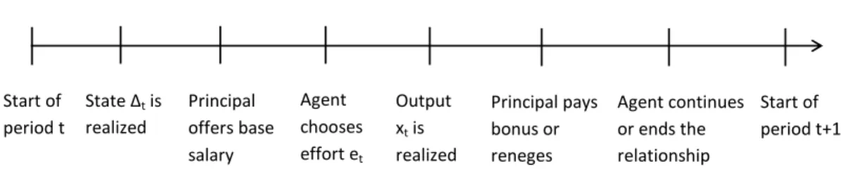
timing of play within each period is summarized in Figure 1 for the case where the agent
participates.
Figure 1: Timing of play within each period
State Δt is
realized
Agent chooses effort et
Output xt is
realized
Principal pays bonus or reneges Start of
period t
Start of period t+1 Agent continues
or ends the relationship Principal
offers base salary
We focus on stationary perfect public equilibria where, on the equilibrium path, period-t
payments and actions depend only on (i) the period-t state, ∆t, and (ii) either period-t
effort, et, if effort is observable, or period-t output, xt, if it is not.14 We can therefore
write S = (sH, sL), denoting the base salary in the high and the low state. If effort is
observable, we can write bonus schedules B(e|H) and B(e|L), which map effort e ∈ [0,1]
to payments in the high and low state respectively. If effort is unobservable, we can write 14Note that period-t output is a noisy signal of period-t effort. Hence, the principal will not condition
B = (bSH, bF H, bSL, bF L), where bSH and bF H denote the bonuses for success and failure,
respectively, when the state is high (andbSL andbF L are defined analogously when the state
is low). Without serious loss, we assume limited liability: S ≥ 0, B ≥ 0, B(e|I) ≥ 0 for
all e∈[0,1],I ∈ {H, L}. We also assume trigger strategies specifying the harshest credible
punishment if the principal deviates from the equilibrium by reneging on a bonus specified
in the relational contract; that is, the agent then ends the employment relationship, takes
his outside option, and the principal earns zero. If the relationship continues to periodt+ 1,
then the players face the same choices as in period t.
We adopt the convention that all compensation not related to agent performance is
cap-tured in the base salary, rather than the bonuses. With observable effort, this amounts to
im-posing mine∈[0,1]B(e|I) = 0,I ∈ {H, L}. Pay-for-luck is then equivalent toB(e|H)6=B(e|L)
for at least some value e ∈ [0,1]; that is, the bonus schedule depends on the realized
state. With unobservable effort, the convention amounts to imposing min(bSH, bF H) =
min(bSL, bF L) = 0. Since offering a higher bonus for failure than for success can never
induce positive effort, it follows that the principal will set bF H =bF L = 0, so we can write
B = (bSH,0, bSL,0) ≡ (bH, bL).15 Pay-for-luck is then equivalent to bH 6= bL; that is, the
bonus for success depends on the realized state. Finally, we assume throughout the analysis
that the agent’s outside options, vH ≥0 and vL ≥0, are sufficiently small for the principal
to always induce participation in each period under the optimal contract; that is, in any
given period, the compensation required to induce the agent to work does not exceed the
expected output produced by working.16
15This convention will pin down the optimal bonuses under formal contracting when the agent’s
partici-pation constraint binds, so where the agent requires a positive base salary. Under relational contracting, the principal would have a strict incentive to abide by this convention to reduce his own temptation to renege on paying the bonuses.
16This assumption rules out the possibility that the bonus varies trivially with the state simply because
3
Theoretical Analysis
3.1
Optimal contracts
We derive the optimal contracts under formal and relational contracting. These contracts
are optimal from the principal’s perspective, in the sense of maximizing expected profits.
Our interest is in generating testable predictions, to ascertain whether there is evidence
of relational contracting in CEO compensation. The testable predictions will follow from
Propositions 1 and 2, derived later in this section. These results show that under formal
con-tracting, bonus payments are independent of the state, whereas under relational concon-tracting,
bonuses may depend on the state and, moreover, the sensitivity of bonuses to the state is
increasing in state persistence.
Deriving these formal results requires taking a stand on whether the principal can observe
agent effort. However, it turns out that Propositions 1 and 2 hold regardless of whether or
not effort is observable. There is therefore no loss in assuming, as we do, that the principal
does not observe effort (see Section 3.2 on robustness for further discussion). We also view
unobservable effort as a natural assumption in the context of CEOs. It implies that agents
will be rewarded for good outcomes more than for bad ones, and that agents acquire strictly
positive surplus, where both implications appear reasonable for CEOs (see Section 3.2 for
further discussion).
We first provide expressions for the expected payoffs of the principal and the agent.
Henceforth, let eH (eL) denote the agent’s optimal effort choice in the high (low) state,
conditional on participation. Suppose that the period-t state is high (i.e., ∆t = ∆). Then
given contract (S, B) and effort choice eH, the principal’s expected period-t profits are
and the agent’s expected payoff is
uH((S, B), eH) = p(eH)bH +sH −C(eH). (2)
Similarly, the principal’s expected profits when the state is low are
πL((S, B), eL) = p(eL)(xS −∆−bL) + (1−p(eL))(xF −∆)−sL, (3)
and the agent’s expected payoff is
uL((S, B), eL) =p(eL)bL+sL−C(eL). (4)
For any t0 ≥ t, define Pt0,t ≡ P(∆t0 = ∆t), which is the probability that the state in
period t0 is the same as the state in period t. Given that P(∆t+1 = ∆t) = θ, we can define
Pt0,t recursively by
Pt0,t =θPt0−1,t+ (1−θ)(1−Pt0−1,t), (5)
fort0 ≥t+ 1, withPt,t= 1. Givenθ >1/2, the correlation between states in any two periods
is positive and increasing in θ.17
The present discounted value of expected profits as of a period when the state is high is
ΠH((S, B), eH, eL) =
∞
X
t=1
δt−1
Pt,1πH((S, B), eH) + (1−Pt,1)πL((S, B), eL)
, (6)
with πH((S, B), eH) given by (1) and πL((S, B), eL) given by (3). Similarly, the present
discounted value of expected profits as of a period when the state is low is
ΠL((S, B), eH, eL) =
∞
X
t=1
δt−1
Pt,1πL((S, B), eL) + (1−Pt,1)πH((S, B), eH)
. (7)
Given a stationary contract and unobservable effort, the agent’s optimal effort choice in
any period t depends only on the incentives offered in that period. Both states are a priori
equally likely, so the principal’s program under formal contracting is
max (S,B) Π =
1
2ΠH((S, B), eH, eL) + 1
2ΠL((S, B), eH, eL), subject to (8)
eH = arg max e∈[0,1]
uH((S, B), e), (9)
eL= arg max e∈[0,1]
uL((S, B), e), (10)
(S, B) = (sH, sL, bH, bL)≥0. (11)
Notice from (2) and (9), and from (4) and (10), that the optimal effort level in a given
state depends only on the bonus offered for success in that state. We can therefore write
eH = e(bH) and eL =e(bL). Recall our assumption that vH and vL are relatively small, so
the principal finds it optimal to induce the agent’s participation in each period, regardless
of the state. That is, the principal will offer a contract that meets the agent’s participation
constraints,
uH((S, B), eH)≥vH, (12)
uL((S, B), eH)≥vL. (13)
Under relational contracting, the principal must have an incentive to pay each bonus
specified under B as promised. Given trigger strategies, the optimal way for the principal
to renege on a bonus is to withhold it completely, so the benefit of reneging equals the
size of the bonus. The cost of reneging is the expected future profits lost when the agent
contracting includes additional, dynamic enforcement constraints,
bH ≤δ
θΠH(sH, sL, bH, bL, eH, eL) + (1−θ)ΠL(sH, sL, bH, bL, eH, eL)
, (14)
bL≤δ
θΠL(sH, sL, bH, bL, eH, eL) + (1−θ)ΠH(sH, sL, bH, bL, eH, eL)
, (15)
where both the cost and benefit from reneging may depend on the current state.
The following lemma shows that the optimal effort level is increasing in the size of the
bonus but at a decreasing rate. As a result, expected profits in any given period will be a
concave function of the promised bonus.
Lemma 1 Let I ∈ {H, L}, and consider the agent’s optimal effort e(bI) in state I,
condi-tional on participating. Then 0 ≤ e(bI) < 1, where the inequality is strict for all bI > 0.
Moreover, e(bI) is unique, with e0(bI)>0 and e00(bI)<0.
We now state our first main result, where superscripts f and r denote formal and
rela-tional contracting, respectively.
Proposition 1 If output is verifiable, the principal will choose formal contracting and offer
the same bonus in both states: bf ≡bf
H =b
f
L >0. If output is nonverifiable so that contracting
is relational, and the agent’s outside options vH and vL are sufficiently small, then the
principal will offer a different bonus in each state when the discount factor is sufficiently
low: for any θ ∈ (1/2,1), there exists δ0 ∈ (0,1) such that 0 < brL < brH ≤ bf for all
δ∈[0, δ0) and brH =bLr =bf for all δ∈[δ0,1].
Proposition 1 says that under relational contracting, the agent may be paid for luck, in
the sense that incentive payments can be positively correlated with the state. In contrast,
pay-for-luck never occurs under formal contracting. The intuition behind the result is as
follows. A large bonus will generate high effort, which increases expected output, but it will
takes into account these two opposing effects by setting the optimal bonus that gives profits
of zero on the margin. Marginal profits are independent of the state, since the state does
not affect the relationship between bonus and effort or the relationship between effort and
success. It follows that the principal offers the same bonus, bf, in both states under formal
contracting.
The difference under relational contracting is that the principal faces a commitment
prob-lem. He would like to offer the same profit-maximizing bonus as under formal contracting,
but he needs an incentive to actually pay this bonus when the agent succeeds. Put another
way, the principal cannot credibly offer a bonus that violates his dynamic enforcement
con-straint. The bonus bf will not be credible if it exceeds the discounted value of expected
future profits, which is what occurs if the discount factor is sufficiently low. With a low
discount factor, the principal can credibly promise a larger bonus in the high state than in
the low state, since the high state offers a looser dynamic enforcement constraint; intuitively,
this is because profits are higher in the high state and states are positively correlated over
time. Total profits are lower than under formal contracting, since marginal profits are strictly
positive at the constrained optimum.18
As Proposition 1 states, correlation between the state and the optimal bonus is a
dis-tinguishing feature of relational contracting compared to formal contracting. This is not
necessarily true for correlation between the state and the optimal base salary. The proof of
Proposition 1 shows that the optimal base salary under formal contracting depends on the
agent’s outside option whenever the participation constraint binds. It follows that a
corre-lation between outside options and state can generate correcorre-lation between state and base
salary. Thus, with formal contracting, the principal may well adjust the base salary over
time for retention purposes, to take into account changes in outside options, but it would 18Notice that neither contract specified in Proposition 1 is first best. This follows from our assumption
always set the same bonus bf >0. This means that variations in the agent’s outside option
cannot explain state-contingent bonuses in our framework.
In the empirical section, we will describe the measures of the components of executive
compensation and our choice of state proxy. The bonus in our theoretical model is any
compensation given after output is realized. Hence, its empirical counterpart can comprise
either cash bonuses or equity grants but not fixed salary. There are differences between cash
bonuses and equity grants; for instance, an equity award need not be immediately cashed
out. However, the data capture the grant-date value of stocks and options, and as long as
the executive perceives the grant-date value as the reward for that period’s outcome, then
our model should apply to equity as well as to cash bonuses.
The following proposition describes how the optimal bonus depends on the degree of
persistence of the state over time.
Proposition 2 Consider the optimal bonuses bf, br
H, and brL given by Proposition 1. Then
bf is independent of θ, whereas br
H −brL is increasing in θ whenever bLr < bf, brH < bf.
Proposition 2 states that the sensitivity of bonus payments to the state with relational
contracting should be higher for firms facing a more persistent state, whereas under formal
contracting the optimal bonus remains the same regardless of the state’s persistence (i.e.,
there is no “pay for luck”). This result accords well with the Informativeness Principle.
When persistence is low, the current state provides little information about future profits.
The principal then faces similar credibility issues across states and offers similar bonuses.
As the state becomes more persistent, the difference in expected future profits between the
high and low states increases. This persistence differentially affects the principal’s credibility
across states and leads to increasingly different bonuses being offered.
The preceding results have the following testable implications. If the state has a strong
positive correlation over time, then bonus payments under relational contracting are more
employment relationship. This means that the difference between the bonus in the high state
and the low state is large. In contrast, in the extreme case where the state is independent
over time, the bonus is insensitive to the state, as it would be under formal contracting.
Thus, persistence of the state is key for empirically detecting relational contracting.
3.2
Alternative Modeling Assumptions
We now briefly describe how our theoretical results on relational versus formal contracting
are robust to relaxing various assumptions. Specifically, we consider the impact of (i) agent
effort being observable; (ii) the presence of more than two states and non-Markov state
transitions; and (iii) agent risk aversion. The overall conclusion in all these cases is that our
main qualitative results continue to hold.19
First, we have derived results showing that Propositions 1 and 2 continue to hold if effort
is observable. That is, the optimal bonus is still independent of the state under formal
contracting but not under relational contracting, and the sensitivity of bonus payments to
the state under relational contracting is increasing in state persistence. Observability of effort
does have some impact on the structure of compensation, as it affects how much information
the principal possesses. When effort is observable, the principal offers the agent a positive
bonus, equal to the cost of effort, for the desired effort level, and offers zero bonus for all
other choices of effort. Doing so allows the principal to capture all surplus under both formal
and relational contracting. But it has no impact on the distinguishing features of relational
contracting versus formal contracting, i.e., the correlation between state and bonus size, and
the relationship between bonus payments and persistence.
Second, our assumptions of a binary state variable and of Markov state transitions help
keep the analysis tractable but are not important for the economic mechanism driving our
results. The positive relationship between state and bonus size under relational
Proposition 1, where we impose the auxiliary assumptions of binary effort and zero outside
options but where we also allow forN ≥2 states and non-Markov transitions.20 This result
shows a positive relationship between state and bonus under relational contracting, but not
under formal contracting, regardless of whether we relax only the assumption of binary state,
only the assumption of Markov transitions, or both assumptions. The crucial feature about
state transitions is not their (non-)Markov character but rather that there be some notion
of persistence. That is, for any particular threshold value of the state, a higher state today
makes it more likely that the state exceeds that particular threshold in the future, captured
in our original modeling framework by the assumption θ >1/2.
Third, another question is whether Proposition 1, which shows that bonus payments are
both smaller and more variable under relational contracting compared to formal contracting,
continues to hold under risk aversion. A risk-averse agent would dislike this variability in
bonuses payments under relational contracting. All else being equal, it might seem plausible
that risk aversion would push up the size of bonus payments under relational contracting
above their level under formal contracting, to compensate the agent for the higher variability.
It turns out that this is not the case. In fact, Proposition 1 continues to hold with agent
risk aversion, so relational contracting continues to yield both smaller and more variable
bonus payments. The economic intuition for this result is that the dynamic enforcement
constraint under relational contracting pushes the principal to implement lower effort than
under formal contracting. This is the case if the agent is risk averse, just as it is if the agent
is risk neutral. Since the agent exerts lower effort under relational contracting, he requires
lower compensation, and hence receives smaller bonuses.21
20The auxiliary assumptions allow us to maintain tractability in a setting where the state variable can
assume arbitrarily many values and where transitions may depend on the entire history of earlier state realizations.
21Moreover, in our setting, the principal has no interest in offering high compensation in both states as a
4
Data and Measures
We extract CEO compensation data from the ExecuComp database from 1992 to 2014.22
Specifically, our sample includes all individuals who have (or have had) the CEO title from the
historical S&P 1500 Index constituent firms, which covers 90% of the market capitalization
in the U.S. stock market. Compensation items include salary, cash bonus, equity-based
payments (i.e., stock and option awards) as well as total compensation (see Table 1 for
summary statistics and data definitions). All compensation variables are deflated to 2009
dollars, and matched to the firm-level financial data to be described shortly. We also include
the CEO’s age, tenure (measured in years from the date the individual became CEO), and
an indicator for the CEO’s first year, because there might be signing bonuses when a CEO
first joins a firm (in which case first-year compensation would be overestimated relative to
what the CEO would normally be paid).
The company financial data are drawn from the CompuStat Annual database from 1987
to 2014. These include a company’s sales, deflated to 2009 dollars, which we use to extract
a firm-specific state proxy. The reason for the lead time prior to 1992 is to increase the data
length for the filtering mechanism to be described shortly.23 Consistent with Bertrand and
Mullainathan (2001), we include the logarithm of shareholder wealth (Mkval) and income
before extraordinary items divided by total assets (IB/AT) to control for firm size and CEO
effort, respectively. In addition, we include market-to-book (MtB) and the leverage ratio
(Lev) to control for growth potential and the free cash flow effect, respectively. We also
include the Gompers–Ishii–Metrick index of corporate governance (G index), where a higher
score indicates more restrictions on shareholder rights or a greater number of anti-takeover
measures, to test the skimming view of pay-for-luck.24
22Comprehensive data on executive compensation in publicly-traded companies are available from 1992,
when the SEC revised its proxy and reporting rules, which required greater disclosure of top executive compensation.
23We drop firms with fewer than ten observations (N ≈ 1800), to achieve reliable filtering results, and
firms with a gap in the sales data (N ≈1300) because gaps are disallowed by the filtering method we use to construct a measure of the state.
The idea behind the construction of our measure of the state variable borrows from the
theory of business cycles, which is concerned with extracting and understanding the cyclical
component of a country’s GDP fluctuations in time series data. The point is to separate
the frequency of business cycles (which typically range from one to several years) from the
nonstationary, long-run trend or high-frequency noise. Although a company’s output is
much smaller than (and different from) a country’s, these time series filtering methods can
be fruitfully applied to companies, and a key point is that there is variation in the nature of
cycles across companies within the same country. For example, even if a company’s business
cycle wavelength is similar in duration to a country’s business cycle, each firm can have a
different amplitude in the time series as well as a different timing of crest and trough. One
considerable advantage of this approach is that the filtering can be applied to each firm’s
time series data, and thus persistent luck need not be common for all firms in a sector or
economy, which allows us to empirically address across-firm comparative statics results such
as Proposition 2.
Specifically, to construct a measure of the state proxy, we apply the Hodrick-Prescott
(HP) filter to the time series of a firm’s annual sales to obtain its cyclical component.25
Numerous studies have shown that the HP filter does a good job of isolating the business
cycle component from long-run trends (e.g., Kydland and Prescott, 1990; Backus and Kehoe,
1992). In considering the relative variance between the cyclical and trend components, we
set the HP smoothing parameter equal to 6.25, following the recent treatment by Ravn and
Uhlig (2002), but also to 100 in a robustness check, following the original suggestion by
Backus and Kehoe (1992). Furthermore, to ensure the robustness of our results, we also
apply a new band-pass filter due to Christiano and Fitzgerald (2003), which is a natural
when we use this variable in our regressions. The G index was published in July 1993, July 1995, February 1998, November 1999, January 2002, January 2004, and January 2006. We imputed the 1992 value with the 1993 value, 1994 with 1995, 1996 and 1997 with 1998, 1999 with 2000, 2001 with 2002, 2003 with 2004, and 2005 with 2006.
25The HP filter smooths a data series y = (y
1, ..., yT)0 by minimizing, over all τ ∈ RT, the function
PT
t=1(yt−τt)2+λP T−1
t=2 (τt+1−2τt+τt−1)2, whereλis a smoothing parameter that for our annual data is
extension of the HP filter.
Figure 2(a) illustrates the HP filtering result (with a smoothing parameter of 6.25) for
the first firm in our sample (i.e., AAR Corporation). The solid line is the original (deflated)
sales data (Sale), and the dotted line nearby is the long-run trend (Sale tr). The cyclical
component (Sale cy) is the deviation of the original data from the trend and is represented
by the dashed line around the horizontal axis. That is, the HP filter leaves the mean of the
original data and the long-run trends almost the same and creates the cyclical component,
which is our state proxy, around mean zero with a sizeable standard deviation. In Table 1,
the HP-filtered state proxy is denoted byStateRU when the HP smoothing parameter is 6.25,
and by StateBK when it is 100. The band-pass filtered state proxy is denoted by StateCF.
Figure 2(b) shows the three different state proxies for AAR Corp. The series tend to comove
but they nonetheless also exhibit some distinct variation.
Finally, we measure the degree of state persistence in two ways. The first measure
is the correlation coefficient between the firm’s state proxy and its once-lagged variable.
Table 1 shows that this correlation (Corr) is positive in the three measurement cases. The
correlation coefficient does not explicitly consider the structure of state dependence assumed
in our model. Hence, we construct an alternative measure of state persistence by fitting
the AR(1) time-series model to each firm’s state proxy and use the coefficient on the
first-lagged dependent variable as another measure of state persistence. Table 1 shows that the
autoregressive coefficient (AR1) is positive, which ensures that the autocorrelation at any
lag is also positive. We estimate this regression individually for every firm, so bothCorr and
AR1 are constant within firms and vary across firms. Thus, when empirically evaluating the
comparative statics result in Proposition 2, our interpretation is that varying θ represents
Figure 2
(a) HP filtering of a firm’s sales
(b) Comparison of three filters
5
Empirical Evidence
5.1
Main results
Our goal in the empirical analysis is to explain the variation in CEO “bonus” compensation
over time and across firms as a function of the state proxy and the persistence of the state
proxy, to evaluate whether the evidence is consistent with the optimal relational contracting
results in Propositions 1 and 2.26 We then test an implication of the skimming view, which 26Our test for relational contracting, which is based on the empirical relationship between the bonus and
implies that pay-for-luck should be stronger in the more poorly governed firms. Because the
G index (a measure of corporate governance) varies relatively little over time, both
predic-tions on state persistence and corporate governance, which are the key effects of interests,
are essentially based on across-firm variation.
Since our theoretical model does not distinguish between cash and equity-based bonuses,
we use both CEO cash bonuses (Bonus) and stock and option awards (Equity) as primary
dependent variables. We also use CEO total compensation (which includes, e.g., deferred
compensation), net of base salary, as a dependent variable (Non Salary=Total−Salary),
which we take as the total measure of CEO compensation that is subject to the board’s
discretion. Our reason for focusing on the above measures of compensation, rather than on
base salary, is that our theoretical model does not provide a clear distinguishing test between
relational and formal contracting when salary is the dependent variable.27
Firstly, Proposition 1 posits that the state has positive direct effects on CEO bonus
compensation under relational contracting. Using the empirical proxies discussed above, we
estimate the following regression to test this prediction:
Yit =β0+β1Stateit+Xitβ+φi+ξt+εit,
where for each CEO-firm combination,Yitis CEOi’s year-tsalary, cash bonus, equity awards,
and total compensation net of salary; Stateit is the cyclical component of firm sales; Xit
contains the aforementioned firm and CEO characteristics and also industry-specific (2-digit
NAICS) linear time trends; φi is a CEO-firm fixed effect; ξt is a year effect; and εit is a
disturbance term that may be correlated within CEO-firm pairs.28
absence of formal contracts does not necessarily imply the existence of relational contracts.
27See the discussion following Proposition 1, describing how under formal contracting, the state has no
impact on bonus size but may have an impact on base salary.
28Because our unit of analysis is a CEO-firm pair, and there is only one CEO per firm per year, the subscript irefers to both the CEO and the firm. Therefore, there are no CEO (or firm) fixed effects identified separately from the CEO-firm fixed effect,φi. The linear trend terms contained inXitareP
22
s=1Indsi×T imet, where Indsi is an indicator for the industry of firmi, andT imetis a linear index measured in increments of single
Specifically, Proposition 1 predicts β1 = 0 under formal contracting, and β1 > 0 under
relational contracting when the dependent variable is Bonus, Equity, and Non Salary, if at
least some firms in the sample have a sufficiently low discount factor. As alluded to above, our
model does not have an unambiguous prediction for the sign ofβ1under formal and relational
contracting when the dependent variable is Salary, but we also present these regression
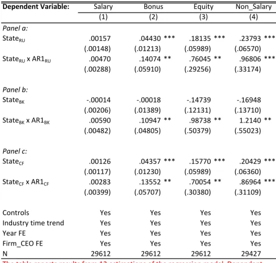
results for the sake of completeness. Estimation results are presented in Table 2, which
reveal that β1 is positive and significant in all columns, except in the first column (Salary),
and in all panels (using different filtering). This is consistent with our basic prediction on
relational contracting. Each measure of CEO “bonus” payments (i.e., cash bonus, equity
awards and total net of salary) is, on average, positively correlated with the firm-specific
state proxy.
Secondly, if the data-generating process is characterized at least in part by relational
contracting, then Proposition 2 posits that firms with a more persistent state should be
driving this result. We test this prediction by using the following interactive specification:
Yit =β0+β1Stateit+β2(Stateit×Corrit) +Xitβ+φi+ξt+εit.
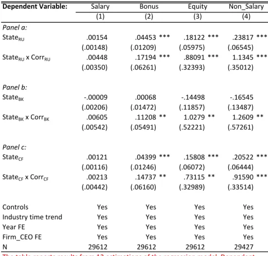
Results from this interactive model are reported in Table 3. The analogous specification
using AR1it, instead of Corrit, as a measure of state persistence is estimated and also
reported in Table 4. In columns (2)-(4), and in all panels (a)-(c), across the two tables,
the coefficient estimates on the interaction term, β2, is positive and statistically significant.
Thus, the results appear supportive of the hypothesis that relational contracting plays a role
in generating the “pay-for-luck” phenomenon in CEO compensation.
The above results are qualitatively and quantitatively robust to the inclusion and
exclu-sion of industry-specific time trends. We also used a log specification where theYit variables
are in logs, and where sales in logs are subjected to the HP filter to derive the state proxy.
sample sizes are roughly two thirds of those reported here, due to zero or negative entries
and the gaps in the time series data that such entries create for the filtering.
5.2
Alternative explanations for pay-for-luck
We now briefly discuss three possible alternative explanations for pay-for-luck and relate
them to our empirical findings. One alternative focuses on changes to CEO outside options.
This view, described in Section 1, is that firms may compensate CEOs for factors beyond
their control not for incentive reasons but rather for retention purposes. If a CEO’s outside
option varies with the state, then compensation might also need to vary with the state so
as to meet the CEO’s participation constraint. The theoretical analysis in Section 3 shows
that this mechanism may generate correlation between the state and the optimal base salary,
but it cannot generate correlation between the state and the optimal bonus under formal
contracting. Given our empirical results, this suggests that varying outside options is unlikely
to explain pay-for-luck in performance pay.
Another alternative explanation relates to liquidity constraints. The idea here is that a
liquidity-constrained firm might use part of any unexpected cash flow (i.e., due to “luck”)
to award CEO bonuses. However, if pay-for-luck were due only to liquidity constraints, then
the impact of the state on CEO compensation should not depend on the state’s persistence;
all that would matter would be current unexpected cash flow. In addition, our empirical
specifications include company financials such as leverage, which plays an important role in
the free cash flow and moral hazard theory (Jensen, 1986), but our results still show that
persistence matters. While these results do not rule out a possible link between liquidity
constraints and CEO compensation, they suggest that such constraints will not be sufficient
to explain the pay-for-luck observed in our data.
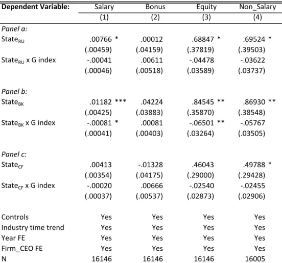
We now turn to the skimming view of executive compensation, which concerns the
forms of pay. We use the G index to estimate the following interactive specification:
Yit=β0+β1Stateit+β2(Stateit×G indexit) +β3G indexit+Xitβ+φi+ξt+εit.
The coefficient of interest is β2. According to the skimming view, β2 is expected to be
positive, because the higher the G index the weaker are shareholder rights. Table 5 displays
the results, where there is no evidence that β2 is positive and significant. If anything, in
some specifications in panel (b), the coefficient estimates on β2 are negative and significant.
Hence, these results are inconsistent with the hypothesis that managerial entrenchment leads
to the observed pay-for-luck phenomenon.
6
Conclusion
We have presented a theoretical contracting model in which formal and relational contracts
have different implications for how bonus payments respond to persistent “luck.” Drawing
on a large sample of publicly-traded companies, and using empirical measures of the
firm-specific state and its persistence, we found evidence consistent with the relational contracting
view of CEO bonus compensation. A reason why firms seem to reward CEOs for luck is that
the expected future value of the employment relationship is larger in good states of the world
than in bad ones, so that the firm’s credibility to pay bonuses (as well as the CEO’s incentive
to exert effort) is higher in good states. Thus, pay-for-luck can be rationalized within the
standard agency framework. In addition to offering an explanation for pay-for-luck that
does not rely on inefficiency, we have provided empirical evidence consistent with the use of
relational contracts in executive compensation.
One policy implication concerns the efficiency losses caused by caps on executive pay.
During the global financial crisis of 2008, when failing firms were getting public bailouts and
of 2009 imposed caps on CEO pay.29 Our analysis implies that under relational contracting,
if a cap on executive bonuses is imposed that binds in some states of the world, then the
distortion the cap causes on pay contracts should vary with state persistence. To the extent
that persistence differs across industries and production environments, this has implications
for how the damage (in terms of distortions in pay contracts) varies across industries. The
caps may be more damaging in industries/settings where the persistence is high, and
pay-for-luck is relatively important, than in settings where the opposite is true. Thus, our analysis
offers an explanation for why the distortions of pay caps may vary across industries and
suggests in which settings these regulations can be expected to have the most bite.
Appendix
Proof of Lemma 1. We prove the case for I = H, where the proof is entirely analogous
for I = L. From (2), the optimal effort eH = arg max e∈[0,1]
uH(bH, e) is uniquely defined by the
first-order condition
p0(eH)bH −C0(eH) = 0, (16)
with the second-order condition, p00(eH)bH −C00(eH) < 0, is satisfied by C00(e) > 0 and
p00(e) <0. Neither condition depends on ∆, meaning that effort only depends indirectly on
the state, through the bonus offered in that state.
IfbH = 0, then (16) reduces toC0(eH) = 0, so thatC0(0) = 0 impliese(0) = 0. If instead
bH >0, then (16) will be violated at eH = 0, since p0(0) > 0 and C0(0) = 0. (16) will also
be violated at eH = 1, since p0(1) is finite and lime→1C0(e) =∞. It follows that eH ∈[0,1)
with eH ∈(0,1) for bH >0.
Implicitly differentiating (16) with respect to bH yields
where we drop the arguments for p0, p00 and C00. Rearranging gives
e0(bH) =
p0 C00−p00b
H .
The second-order condition and p0 >0 then imply e0(bH)>0. Now implicitly differentiating
(17) with respect to bH yields
p000(e0(bH))2bH +p00e00(bH)bH + 2p00e0(bH)−C000(e0H(bH))2−C00e00(bH) = 0,
and rearranging gives
e00(bH) =
(p000bH −C000)(e0(bH))2+ 2p00e0(bH) C00−p00b
H
.
The numerator is strictly negative by p000 ≤ 0, C000 ≥ 0, p00 < 0 and e0(bH) > 0. The
denominator is strictly positive by the second-order condition. It follows thate00(bH)<0.
Proof of Proposition 1. Relational contracting only differs from formal contracting
through additional constraints (14) and (15). It follows immediately that the principal will
use formal contracting whenever it is feasible, so whenever output is verifiable.
Suppose for now that the optimal contract always induces the agent to participate,
re-gardless of the realization of the state. By (6) and (7), Π = 12ΠH + 12ΠL is increasing in πH
and πL, where specifically
ΠH(sH, sL, bH, bL) =
∞
X
t=1
δt−1Pt,1
πH(sH, bH) +
∞
X
t=1
δt−1(1−Pt,1)
πL(sL, bL), (18)
and
ΠL(sH, sL, bH, bL) =
∞
X
t=1
δt−1Pt,1
πL(sL, bL) +
∞
X
t=1
δt−1(1−Pt,1)
Write (1) as
πH(sH, bH) = p(e(bH))(xS−xF −bH)−sH +xF + ∆, (20)
and write (3) as
πL(sL, bL) =p(e(bL))(xS−xF −bL)−sL+xF −∆. (21)
The first- and second-order conditions for profits with respect to bonus are independent
of base salary and are the same in both states. Therefore, we write these conditions as
π0(b) = 0, π00(b)<0, with
p0(e)e0(b)(xS−xF −b)−p(e) = 0, (22)
p00(e)e02+p0(e)e00(b)
(xS−xF −b)−2p0(e)e0(b)<0.
The first-order condition is violated at b = 0, where π0(0) > 0, since e(0) = 0 and
e0(0) >0 by Lemma 1, and since p(0) = 0 andp0(0) >0. It is also violated for b≥xS−xF,
whereπ0(b)<0, since e(b)>0 ande0(b)>0 by Lemma 1, and since p(e)>0 andp0(e)>0.
The second-order condition is satisfied for all b < xS−xF, since e00(b)<0 by Lemma 1,
and sincep00(e)<0. It follows thatbf ≡bfH =bfL= arg max b≥0
πH(sH, b) = arg max b≥0
πL(sL, b)∈
(0, xS −xF) is uniquely defined by (22).
The optimal bonus bf is independent of the state and the base salary. Thus, the only
reason for the principal to offer a positive base salary in either state is to induce agent
participation. This means that the optimal contract under formal contracting isS∗ = (0,0)
and B∗ = (bf, bf), if this contract satisfies participation constraints (12) and (13). More
generally the optimal contract is S= (max(vH −u(S∗, B∗),0), max(vL−u(S∗, B∗),0)) and
B = (bf, bf). That is, the principal only offers a positive base salary s
the participation constraint bind.
The principal will induce participation in both states if doing so yields non-negative
profits under the optimal contract: πH(sH = 0, bf) −max(vH − u(S∗, B∗),0) ≥ 0 and
πL(sL = 0, bf)−max(vL−u(S∗, B∗),0)≥0, with πH(sH = 0, bf) given by (20) and πL(sL=
0, bf) given by (21). These inequalities reduce to π
H(sH = 0, bf)≥0 and πL(sL = 0, bf)≥0 when vH =vL = 0, sinceu(S∗, B∗)≥0 follows from the fact that the agent can always earn
zero payoff by exerting zero effort. Note that the principal could always earn positive profits
by offering zero bonus: ∆< xF impliesπL(sL= 0, bL= 0) >0 andπH(sH = 0, bH = 0) >0;
hence πH(sH = 0, bf)> 0 and πL(sL = 0, bf)> 0 follow by the optimality of bf. Thus, the
principal finds it optimal to always induce participation if and only ifvH ∈[0, vH] andvL∈
[0, vL], wherevH ≡πH(sH = 0, bf) +u(S∗, B∗)>0 and vL≡πL(sL= 0, bf) +u(S∗, B∗)>0.
We now turn to the optimal contract under relational contracting. We will consider
contracts with zero base salary, sH = sL = 0, and derive the optimal bonuses brH and b r L, supposing that the participation constraints (12) and (13) are satisfied. We will then argue
that the contract thus derived is in fact optimal and satisfies the participation constraints
when outside options vH ≥0 and vL≥0 are sufficiently small.
Denoting b =bL, and substituting (6) and (7) into (14) gives
bH ≤δ
∞
X
t=1
δt−1[θPt,1+ (1−θ)(1−Pt,1)]πH(bH) +
∞
X
t=1
δt−1[(1−θ)Pt,1+θ(1−Pt,1)]πL(b) !
,
(23)
where πH(bH) is evaluated at e(bH) and πL(b) is evaluated at e(b).
Similarly, denoting b=bH, and substituting (6) and (7) into (15) gives
bL ≤δ
∞
X
t=1
δt−1[θPt,1+ (1−θ)(1−Pt,1)]πL(bL) +
∞
X
t=1
δt−1[(1−θ)Pt,1 +θ(1−Pt,1)]πH(b) !
,
(24)
where πL(bL) is evaluated at e(bL) and πH(b) is evaluated at e(b).
br
L ≤bf. If either inequality were violated, then setting (bf, bf) instead of (brH, brL) would yield strictly higher profits Π = 12ΠH +12ΠL by (18) and (19), where πH0 (b)<0 andπ
0
L(b)<0 for b > bf. Moreover, setting (bf, bf) instead of (brH, brL) would decrease the left-hand side and
increase the right-hand side of both (23) and (24). Hence, if (23) and (24) are satisfied by
(br
H, brL), they must also be satisfied by (bf, bf).
The constraint (23) holds strictly at bH = 0, since πH(0) = xF + ∆ > 0 by (20) and
πL(0) = xF −∆ > 0 by (21). The right-hand side of (23) is concave in bH on [0, bf] while
the left-hand side is linear. It follows that for any given b, there is at most one value of
bH ≤bf for which (23) binds, and this value (if it exists) will be strictly positive. Define the
function bH(b) on domain [0, bf] as the minimum of this value andbf. Since π0H(bH)>0 for
bH ∈[0, bf), the optimal bonus in the high state givenbL=b is precisely bH(b).
By the same reasoning, for any b, there is at most one value of bL ≤ bf for which (24)
binds, and this value (if it exists) will be strictly positive. Define the function bL(b) on
domain [0, bf] as the minimum of this value and bf. Since πL0 (bL) > 0 for bL ∈ [0, bf), the
optimal bonus in the low state given bH =b is preciselybL(b).
The optimal bonus pair (br
H, brL) must satisfybH(bL(brH)) = brH, withbrL=bL(brH). Define the correspondence f(b) by f(bH(b))≡b, so that f(b) is the inverse of bH(b). Then (brH, brL)
must also satisfy bL(brH) = f(brH), again with brL = bL(brH). Geometrically, f(b) is the
reflection of bH(b) about the 45 degree line, and (bHr , brL) lies at an intersection of f(b) and
bL(b).
The function bL(b) is continuous, with domain [0, bf] and range [bL(0), bL(bf)], where
bL(0) >0 and bL(bf)≤bf. The function bH(b) is continuous, with domain [0, bf] and range
[bH(0), bH(bf)], where bH(0) > 0 and bH(bf) ≤ bf. It follows that its inverse f(b) is also
continuous, with domain [bH(0), bH(bf)] and range [0, bf], withf(bH(0)) = 0.
We now show that b0H(b)>0 andb00H(b)<0 whenever bH(b)< bf, and thatb0L(b)>0 and
b00L(b)<0 wheneverbL(b)< bf. The fact thatb0H(b)>0 implies that the correspondencef(b)
is single valued for all b < bf, with f0(b) > 0, where b00
H(b) < 0 implies f
that bH(b) < bf, so that (23) binds at bH < bf, and fix the value of bH. The right-hand
side of (23) is increasing in b, since π0L(b) > 0 for all b < bf. It follows that (23) no longer
binds after a marginal increase in b. Since the left-hand-side of (23) is convex in bH and the
right-hand-side is concave, it follows that b0H(e)>0, and hence f0(b)>0.
Similarly, suppose that bL(b) < bf, so that (24) binds at bL < bf, and fix the value
of bL. The right-hand side of (24) is increasing in b, since πH0 (b) > 0 for all b < bf. It
follows that (24) no longer binds after a marginal increase inb. Hence,b0L(b)>0. Implicitly
differentiating (23) with respect to b and rearranging gives
b0H(b) =
δ
P∞ t=1δ
t−1
(1−θ)Pt,1+θ(1−Pt,1)
π0L(b)
1−δ
P∞ t=1δt−1
θ Pt,1+ (1−θ)(1−Pt,1)
π0
H(bH)
. (25)
The numerator and the denominator of (25) are both positive byπL0 (b)>0 andb0H(b)>0.
An increase in b will decrease the numerator since π00L(b)<0, and increase the denominator
sinceb0H(b)>0 andπH00(bH)<0. This means thatb00H(b)<0 wheneverbH(b)< bf. Implicitly
differentiating (24) with respect to b and rearranging yields
b0L(b) =
δ
P∞ t=1δ
t−1
(1−θ)Pt,1+θ(1−Pt,1)
πH0 (b)
1−δ
P∞ t=1δt−1
θPt,1+ (1−θ)(1−Pt,1)
π0
L(bL)
. (26)
The numerator and the denominator of (26) are both positive byπH0 (b)>0 andb0L(b)>0.
An increase in b will decrease the numerator since π00H(b)<0 and increase the denominator
since b0L(b) > 0 and π00L(bL) < 0. This means that b00L(b) < 0 whenever bL(b) < bf, so that
f00(b)>0, as required.
Given continuity on their respective domain and range, there exists some br
H ∈(0, bf] for which bL(brH) = f(brH), so where the curves bL(b) and f(b) intersect. Since bL(b) is concave
whilef(b) is strictly convex, this point of intersection is unique. It defines the optimal bonus
pair, br
To compare the size of the two bonuses, note that br
L = brH holds if and only if bL(b) and f(b) intersect on the 45 degree line. This is the case if bL(b) = b implies f(b) = b or,
equivalently, bH(b) = b. In contrast, bLr < brH holds if and only if bL(b) intersects the 45
degree line before f(b) does. This is the case if bL(b) = b implies f(b) < b or, equivalently,
bH(b)> b.
We now prove that bH(b) = bf whenever bL(b) = bf and that bH(b) > bL(b) whenever
bL(b)< bf. It is sufficient to show that (23) holds strictly whenever (24) is satisfied.
Substi-tuting (20) and (21) into (23) and (24) shows the latter two constraints are symmetric with
respect to bH and bL except for terms involving ∆.
Specifically, the expression δ(2θ−1)P∞ t=1δ
t−1(2P
t,1−1)∆ enters with a positive sign on the right-hand side of (23) and a negative sign on the right-hand side of (24). We claim that
Pt,1 >1/2 for allt≥1 which, together with θ >1/2, implies this expression is itself strictly
positive. Hence, (23) holds strictly whenever (24) is satisfied.
We prove the claim Pt,1 > 1/2 by induction. Recall from (5) the recursive definition
P1,1 = 1 and Pt,1 = θPt−1,1 + (1 −θ)(1 − Pt−1,1) for all t ≥ 2. Clearly Pt,1 > 1/2 for
t = 1. Now fix t0 ≥ 2, and suppose that Pt,1 > 1/2 for all t = 1, . . . t0 −1 and write
Pt0,1 = θPt0−1,1 + (1−θ)(1−Pt0−1,1). The induction hypothesis implies Pt0−1,1 > 1/2 and
(1−Pt0−1,1)<1/2. Combined with θ >1/2, this yields Pt0,1 >1/2.
Note that the right-hand side of (24) increases without bound as δtends to 1. Fixb =bf
and defineδ0 ∈(0,1) as the value ofδfor which (24) binds. Then (24) holds for all b∈[0, bf]
if and only if δ ∈[δ0,1]. Therefore, we havebrL< brH for all δ ∈(0, δ0) and brL=brH =bf for
allδ ∈[δ0,1].
We now conclude by showing that the contract with zero base salary, sH = sL = 0,
along with bonus (br
H, brL) is in fact optimal if it satisfies participation constraints (12) and (13), and that these constraints are satisfied when outside options vH ≥ 0 and vL ≥ 0 are
sufficiently small.
de-creasing in sH and sL, throughπH(sH, bH) andπL(sL, bL). This means that holding bonuses
and agent effort constant, both constraints are more difficult to satisfy when sH > 0 or
sL >0 than when sH =sL = 0. Recall from (9) and (10) that the agent’s optimal effort was
independent of sH and sL. Hence, the contract in question is optimal if it induces the agent
to participate.
Lemma 1 showed that the agent’s payoff is strictly concave in effort, with optimal effort
e(b) > 0 for any b > 0, so in particular e(bHr ) > 0 and e(brL) > 0. Hence, expected payoffs
u(0, brH) and u(0, brL) are strictly greater than zero, which is what the agent could earn in
each state by exerting zero effort. It then follows from (12) and (13) that the contract in
question satisfies both participation constraints for vH and vL sufficiently small.
Proof of Proposition 2. The bonus bf under formal contracting is defined by the
first-order condition (22), which is independent ofθ. As in the proof of Proposition 1, define
the optimal bonus pair (brH, brL) by bH(bL(brH)) = brH or, equivalently, bL(brH) = f(brH), with
brL =bL(brH).
We first show that ∂bH
∂b < ∂bL
∂b for any b such that bL(b)< b
f and b
H(b)< bf. Recall that ∂bH
∂b and
∂bL
∂b are given by expressions (25) and (26). Since π
0
H(b) = π
0
L(b), these expression only differ by the terms π0H(bH) and π0L(bL) in their respective denominators. Combining
bH(b) > bL(b) from the proof of Proposition 1 with πH00(b) = π
00
L(b) < 0 for all b < bf gives πH0 (bH)< πL0(bL), so that (25) and (26) imply ∂b∂bH < ∂b∂bL.
We now show that ∂bH
∂θ >0 whenever b < bH(b)< b
f and that ∂bL
∂θ <0 wheneverbL(b)< b < bf. Suppose that (23) binds at bH ∈(b, bf), and fix the value of bH. Differentiating the
right-hand side of (23) with respect to θ gives
δ
∞
X
t=1
δt−1 2Pt,1−1 +Pt,01(2θ−1)
(πH(bH)−πL(b))
, (27)
where Pt,01 denotes the derivative of Pt,1 with respect toθ.