STATISTICAL ESSAYS MOTIVATED BY GENOME-WIDE ASSOCIATION STUDY
Ling Wang
A dissertation submitted to the faculty of the University of North Carolina at Chapel Hill in partial fulfillment of the requirements for the degree of Doctor of Philosophy in the
Department of Statistics and Operations Research.
Chapel Hill 2015
Approved by:
Haipeng Shen
Guang Guo
Chuanshu Ji
Edward Carlstein
c 2015 Ling Wang
ABSTRACT
LING WANG: STATISTICAL ESSAYS MOTIVATED BY GENOME-WIDE ASSOCIATION STUDY.
(Under the direction of Haipeng Shen and Guang Guo.)
Genome-wide association studies (GWAS) have been gaining popularity in recent years,
and have generated a lot of interests in statistics. In this dissertation, motivated by GWAS, we
develop statistical methods to identify significant Single-Nucleotide Polymorphisms (SNPs)
that are associated with certain phenotype traits of interest. Usually in GWAS, the number of
SNPs are much larger than the number of individuals. Hence identifying significant SNPs and
estimating their effects is a high-dimensional selection and estimation problem, or sometimes
referred to as the largepand smalln(pn) paradigm.
In this research, we propose three approaches to estimate the proportion of SNPs that are
significantly associated with the trait of interest in GWAS, as well as the distribution of their
effects. The first one (Chapter 2) extends the earlier work by Yang et al. [2011a] that models
the SNP effects as random effects in a linear mixed model. We instead assume a mixture
prior on the random effects, which consists of a pointmass at zero, for those non-significant
SNPs, plus a normal component for those significant SNPs. We develop a fast Markov Chain
Monte Carlo (MCMC) algorithm to estimate the model parameters. The proposed algorithm
reduces the computation time significantly by calculating the posterior conditional on a set
of latent variables, that index whether the SNPs are associated with the trait of interest or not.
In the second project (Chapter 3), we relax the prior distribution to a mixture point mass
plus a non-parametric distribution. Two types of sieve estimators are proposed based on a
least squares (LS) method for probability distributions under the framework of measurement
empir-ical distribution/characteristic functions and the model distribution/characteristic functions,
respectively. In addition, we use roughness penalization to improve the smoothness of the
resulting estimators and reduce the estimation variance. We also establish the asymptotic
properties of the estimators.
In the third project (Chapter 4), we propose an estimator for the normal mean problem
that can adapt to the sparsity of the mean signals as well as incorporate correlation among
the signals. The estimator effectively decomposes the arbitrary covariance matrix of the
ob-served signals into two parts: principal factors that derive the strong dependence and weakly
dependent error terms. By taking out the largest common factors, the correlation among the
signals are significantly weakened. An automatic nonparametric empirical Bayesian method
is then used to estimate the sparsity and identify the nonzero means.
We apply all the proposed estimators to the Framingham Heart Study data to identify
the SNPs that are associated with the body mass index (BMI). The estimators are able to
identify several SNPs on theFTOgene, which have been shown to be associated with BMI
ACKNOWLEDGMENTS
This is great opportunity to pay my deepest gratitude to my advisors, Professor Haipeng
Shen and Professor Guang Guo, whose guidance, encouragement and support enabled me to
enjoy my research and complete my dissertation work. Prof. Shen helped me in learning a lot
of knowledge in Statistics and provided many opportunities for various kinds of collaborative
research. Prof. Guo led me into the current research field of Human Genetics and gave me
great support in my research.
From them, I improved myself a lot in getting motivated from real problems, in
formu-lating scientific problems and developing novel methods. Thanks to their stimuformu-lating
sug-gestions, encouragement and complete support through my time at Chapel Hill. Beyond and
above their obligations as a thesis advisors, they have been an integral advocate to any and
all of my potential future pursuits.
I also wish to express my sincere appreciation to the committee members, Professor
Ed-ward Carlstein, Professor Chuanshu Ji, Professor J. S. Marron, and Professor Richard Smith,
for their valuable comments and suggestions on this dissertation.
For the projects reported in Chapters 2 and 3, the author gratefully thanks the reviewers
ofBMC GenomicsandJournal of the Korean Statistical Society for their helpful comments and constructive suggestions.
Finally, I would like to thank my husband Zongqiang Liao for everything he has done for
me as a family. This dissertation would not have been possible without his love, support, and
TABLE OF CONTENTS
LIST OF TABLES . . . viii
LIST OF FIGURES . . . ix
CHAPTER 1: INTRODUCTION . . . 1
1.1 Background on Genome-Wide Association Study . . . 1
1.2 Background on Genome-Wide Complex Trait Analysis . . . 2
1.3 Outline . . . 3
CHAPTER 2: MIXTURE SNPS EFFECT ON PHENOTYPE IN GENOME-WIDE ASSOCIATION STUDIES . . . 7
2.1 Background . . . 7
2.2 Methods . . . 10
2.3 Results and Discussion . . . 13
2.3.1 Simulation Studies . . . 13
2.3.2 Real Data Set Results . . . 16
2.4 Conclusion . . . 21
CHAPTER 3: LEAST SQUARES SIEVE ESTIMATION OF MIXTURE DISTRIBUTIONS WITH BOUNDARY EFFECTS. . . 26
3.1 Introduction . . . 26
3.2 The Model and The Estimators . . . 28
3.2.1 The Model . . . 28
3.2.2 LS Based on Cumulative Distribution Functions . . . 30
3.2.3 LS Based on Characteristic Functions . . . 31
3.2.4 Penalization on Roughness . . . 32
3.4 Simulation Studies . . . 35
3.4.1 Study 1: One Point Mass, Correct Specification of Measurement Error Distribution . . . 35
3.4.2 Study 2: One Point Mass, Misspecified Error Distribution . . . 39
3.4.3 Study 3: One Point Mass, Misspecified Variance of the Error Distribution . . . 41
3.4.4 Study 4: Two Point Masses . . . 42
3.5 Application to the Framingham Heart Study Data . . . 42
3.5.1 Data Description . . . 44
3.5.2 Analysis Results . . . 44
3.6 Conclusion . . . 46
CHAPTER 4: MIXTURE PRIOR FOR SPARSE SIGNAL WITH DEPENDENT COVARIANCE STRUCTURE . . . 48
4.1 Introduction . . . 48
4.2 Model and Estimation . . . 51
4.2.1 Model . . . 51
4.2.2 Principal Factor Approximation . . . 52
4.2.3 Empirical Bayesian Estimation . . . 54
4.3 Simulation Studies . . . 58
4.4 Real Data Analysis . . . 63
4.4.1 Data Description . . . 63
4.4.2 Distribution of marginal SNPs Effects . . . 64
4.4.3 Analysis Results . . . 64
4.5 Conclusion . . . 66
APPENDIX 1: APPENDIX TO CHAPTER 3 . . . 67
LIST OF TABLES
2.1 Example 1 - Simulation Results with number of SNPs as 10,000 . . . 15
2.2 Example 2 - Simulation Results with Number of SNPs as 100,000 . . . 17
2.3 Example 2 - Detection Rate using HBM with Number of SNPs as 100,000 . . . 17
2.4 Real Data Estimation Results using HBM and MLM . . . 19
2.5 Per Allele Change in BMI for Association SNPs Identified by HBM . . . 22
2.6 The Framingham Heart Study: PVE Estimation Using Propor-tion of SNPs Based on P-value Thresholda . . . 23
2.7 The HBM Algorithm . . . 25
3.8 Bias, Standard Deviation and MSE of The Five Estimators: ML, LS-cdf, LS-chf, Penalized LS-cdf and Penalized LS-chf . . . 38
3.9 Comparison of Robustness of the ML, LS-cdf and LS-chf Estimators . . . 40
3.10 Study 4: Comparison of LS-cdf and LS-chf with Two Point Masses . . . 43
4.11 Different Distributions ofXused in Simulation Studies . . . 58
LIST OF FIGURES
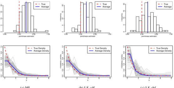
3.1 Figure 1. (Study 1: One Point Mass, Correct Specification
of Measurement Error Distribution)Histogram of ML, LS-cdf
and LS-chf estimators . . . 37
3.2 Figure 2. (Study 1: One Point Mass, Correct Specification of
Measurement Error Distribution) The penalized LS-cdf estimators. . . 37
3.3 Figure 3. (Study 1: One Point Mass, Correct Specification of
Measurement Error Distribution) The penalized LS-chf estimators. . . 37
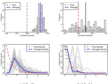
3.4 Figure 4. (Study 2: One Point Mass, Misspecified Error
Dis-tribution) The histogram of LS-cdf and LS-chf estimators. . . 40
3.5 Figure 5. (Study 3: One Point Mass, Misspecified Variance of
the Error Distribution) The histogram of LS-cdf and LS-chf estimators. . . 41
3.6 Figure 6. (Study 4: Two Point Masses) The histogram of
LS-cdf and LS-chf estimators. . . 42
3.7 Figure 7. The sieve estimators and penalized sieve density
estimators based on LS-chf and LS-cdf with application using
the Framingham Heart Study data set. . . 45
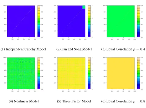
4.8 Figure 1. Heatmap for the Covariance of the Error TermsZ. . . 59
4.9 Figure 2. Estimated wand MSE by DepEB and EB for
CHAPTER 1: INTRODUCTION
1.1 Background on Genome-Wide Association Study
The motivation of this dissertation mainly comes from genome-wide association studies
(GWAS) which have been gaining popularity in recent years. In genetic epidemiology, a
GWAS is an examination of genetic variants in a sample of individuals to see whether there
exists any variant associated with a trait. Typically, single-nucleotide polymorphisms (SNPs)
are used as genetic variants and major diseases are considered as traits. The main purpose of
GWAS is to find the association between genetic variants and traits.
The most common approach of GWAS is the case-control setup which compares two
large groups of individuals: one healthy control group and one case group affected by a
dis-ease. All individuals in each group are genotyped for the majority of commonly known SNPs.
Each of these SNPs is then investigated to see whether the allele frequency is significantly
altered between the case and the control groups. If certain genetic variations are found to be
significantly more frequent in people with the disease compared to people without disease,
the variations are said to be “associated” with the disease. The associated genetic variations
can serve as powerful pointers to the region of the human genome where the disease-causing
problem resides. If the phenotype of interest in continuous variable, such as BMI,
Choles-terol level and heart rate, each SNP is regressed with the phenotype to get the marginal effect
of SNPs on the phenotype. To account for multiple testing, Bonferroni correction was used
and only those SNPs withp <0.05/(number of SNPs) were considered significantly related with the phenotype (Speliotes et al. [2010] and Visscher [2008]). There are several studies
de-veloped an efficient Monte Carlo approach to evaluate error rates for arbitrary test statistics
in genome studies. Fan et al. [2012a] proposed a dependence-adjusted procedure that is more
powerful than the fixed-threshold as in Bonferroni procedure.
In GWAS, the associated variants themselves may not directly cause the disease. They
may just be “tagging along” with the actual causal variants. For this reason, researchers often
need to take additional steps, such as sequencing DNA base pairs in that particular region of
the genome, to identify the exact genetic change involved in the disease.
The first successful GWAS was conducted by Klein et al. [2005] which investigated
the association of SNPs with age-related macular degeneration (AMD). One limitation of
GWAS such as the one in Klein et al. [2005] is that although the control for multiple testing
through Bonferroni correction is able to maintain the familywise error rate (FWER) under
0.05, some significant SNPs predicting traits might be excluded from further analysis be-cause of the extremely small p-value threshold used in Bonferroni correction. It has been
noted that “the GWA approach can be problematic because the massive number of
statisti-cal tests performed presents an unprecedented potential for false-positive results” by Pearson
and Manolio [2008].
Furthermore, GWAS has been criticized for unable to explain much genetic variation/heritability
in the population. SNPs identified by GWAS explain only a small fraction of the genetic
vari-ation because of the strict significance thresholds when testing individual SNPs. For example,
Visscher [2008] discovered 54 loci associated with height which only explained 5% of the
heritability; Speliotes et al. [2010] found 32 loci associated with BMI which only explained
1.45%of the variance in BMI.
1.2 Background on Genome-Wide Complex Trait Analysis
To resolve the issue that traditional GWAS can explain only a small fraction of the
Complex Trait Analysis (GCTA) and its software. The key assumption behind GCTA is that
the SNP effects are random, which follow a normal distribution. Yang et al. [2011a] fit the
effects of all SNPs as random in a mixed linear model (MLM):
y=Xβ+W u+ (1.1)
whereyis ann×1vector of traits.β is a vector of fixed effects such as sex, age, and/or one or more eigenvectors from principal component analysis (PCA),uis a vector of SNP effects
withu ∼ N(0, σ2
u), and ∼ N(0, σ2). W is a standardized genotype matrix with the ijth
elementwij = (xij −2pi)/
p
2pi(1−pi), wherexij is the number of copies of the reference
allele for theithSNP of thejthindividual andp
iis the frequency of the reference allele. The
variance ofyisW W0σ2
u+Iσ2.
By assuming that the SNP effects (u) follow a normal distribution N(0, σ2
u), GCTA is
able to estimate the variance explained by all the SNPs on the whole genome for a complex
trait, rather than testing the association of any particular set of SNPs to the trait. Yang et al.
[2010a] found that 45% of height can be explained by all the SNPs, which is significantly higher than the previous GWA studies. However, it is biologically unrealistic to expect nearly
100%of the SNPs to have an effect on a phenotype of interest. This motivates the dissertation research, which aims to select the set of SNPs that are associated with a phenotype.
1.3 Outline
The first project (Chapter 2) in my dissertation extends the model in Yang et al. [2011a]
by assigning a prior on the random effects so that they follow a mixture of point mass at zero
and a normal distribution. The model used in Yang et al. [2011a] assumes that all SNPs are
associated with the phenotypes of interest. However, it is more common that only a small
very small effects. To incorporate this feature, we propose an efficient Hierarchical Bayesian
Model (HBM) that extends the existing mixed models to enforce automatic selection of
sig-nificant SNPs. The HBM models the SNP effects using a mixture distribution of a point mass
at zero and a normal distribution, where the point mass corresponds to those non-associative
SNPs. We estimate the HBM using Gibbs sampling. The estimation performance of our
method is first demonstrated through two simulation studies. We make the simulation setups
realistic by using parameters fitted on the Framingham Heart Study (FHS) data. The
simula-tion studies show that our method can accurately estimate the proporsimula-tion of SNPs associated
with the simulated phenotype and identify these SNPs, as well as adapt to certain model
mis-specification than the standard mixed models. In addition, we analyze data from the FHS
and the Health and Retirement Study (HRS) to study the association between Body Mass
Index (BMI) and SNPs on Chromosome 16, and replicate the identified genetic associations.
The results demonstrate that the HBM and the associated estimation algorithm offer a
pow-erful tool for identifying significant genetic associations with phenotypes of interest, among
a large number of SNPs that are common in modern genetics studies.
In the second project (Chapter 3), two types of sieve estimators based on a least squares
(LS) method are proposed to solve the sparse high-dimensional estimation problems. The
motivation of this study comes from the real application of Chapter 2 which finds that the
mixture prior distribution for random effects as point mass plus normal distribution might be
too restrictive. In this study, we relax the prior distribution as a mixture of point masses and
a nonparametric distribution under the framework of measurement error models. We obtain
two types of LS sieve estimators through minimizing the distance between the empirical
distribution/characteristic functions and the model distribution/characteristic functions. Lee
et al. [2013] also estimated the distribution using maximum likelihood (ML) within each
sieve. The LS estimators outperform the ML sieve estimator by Lee et al. [2013] in several
squared error; 3) The characteristic function based LS estimator is more robust against
mis-specification of the error distribution. We also use roughness penalization to improve the
smoothness of the resulting estimators and reduce the estimation variance. As an application
of our proposed LS estimators, we use the Framingham Heart Study data to investigate the
distribution of genetic effects on body mass index. Finally asymptotic properties of the LS
estimators are investigated.
The third project (Chapter 4) extends the earlier projects by allowing the error terms in
the normal mean model to have an arbitrary dependent structure. The motivation comes from
traditional GWAS, where marginal regressions are fitted using the phenotype against each
SNP respectively, and then researchers select the SNPs with the most significant marginal
effects. Intuitively, the marginal effects of the SNPs on the trait are correlated and sparse.
To identify the SNPs associated with the trait, we propose an estimation method for the
nor-mal mean problem that can adapt to the sparsity of the signals as well as take correlation
among the signals into consideration. The proposed method effectively decompose arbitrary
dependent covariance matrix of observed signals into two parts: principal factors that derive
the strong dependence and weakly dependent error terms. The correlation among the signals
are significantly weakened after taking out the largest common factors. Based on the
likeli-hood of the signals removing the strong dependence, we use empirical Bayesian method to
estimate the sparsity in the signals. As demonstrated in the simulated examples with several
different dependent structures of signals, our estimate of sparsity compares favorably with
Raykar and Zhao [2010]’s method which considers the signals are identical independent
dis-tributed. Furthermore, our approach is illustrated by GWAS data set and successfully identify
the SNPs onFTOgene associated with body mass index (BMI).
Chapter 5 reports a collaborative study where we investigate how the human genome as a
whole interacts with historical period, age and physical activity to influence BMI using GCTA
test the hypothesis whether the influence of human genome as a whole on obesity depends on
historical period, age, and level of physical activity. The hypothesis testing based on Pitman’s
test, permutation Pitman’s test, F test, and permutation F test produce three sets of significant
findings. First, the genomic influence on BMI is substantially larger after the mid-1980s than
in the few decades before the mid-1980s within each age group of 21-40, 41-50, 51-60 and
>60. Second, the genomic influence on BMI weakens as one ages across the life course or
the genome influence on BMI tends to be more important during reproductive ages than after
reproductive ages within each of the two historical periods. Third, within the age group of
21-50 and not in the age group of >50, the genomic influence on BMI among physically
active individuals is substantially smaller than the influence on those who are not physically
CHAPTER 2: MIXTURE SNPS EFFECT ON PHENOTYPE IN GENOME-WIDE ASSOCIATION STUDIES
2.1 Background
Genome-wide association studies (GWAS) have successfully identified genetic loci
asso-ciation with complex diseases and other traits. SNPs identified by traditional GWAS can only
explain a small fraction of the heritability, due to the strict multiple-comparison significance
requirement when testing each SNP individually. For example, Visscher [2008] discussed
54 loci associated with height which only explained5% heritability; Speliotes et al. [2010] described 32 loci associated with Body Mass Index (BMI) which explained1.45%of the vari-ance in BMI. More recently, Yang et al. [2011a] used mixed linear models (MLM) to
simul-taneously take into account all the SNPs, which is shown to alleviate the missing-heritability
issue.
In this study, we extend the work of Yang et al. [2011a] to identify the subset of SNPs
that are significantly associated with the phenotype of interest, instead of assuming all the
SNPs are associative, through a Hierarchical Bayesian model (HBM). Similar to Yang et al.
[2011a], all SNPs are considered simultaneously to estimate the heritability, instead of one
by one as in the traditional GWAS, hence our HBM also helps to capture missing heritability.
Different from the authors in Yang et al. [2011a], we assume that the SNP effects are
dis-tributed as the mixture of a point mass at zero, for those non-associative SNPs and a normal
distribution for those associative SNPs.
Our proposed Hierarchical Bayesian model (HBM) can be represented using the
[2011a]: Yis then×1response vector which corresponds to the individuals’ phenotype in our study,Xis the design matrix for the fixed effects,Wis the standardized genotype matrix,
and the vectorb contains the N SNP random effects, where the jth element is the random
effect corresponding to thejth SNP and is assumed to follow the mixture distribution as in
(2.3), depending on the latent indicatorIj,j = 1, . . . , N:
Y=Xβ+Wb+, (2.2)
where
bj
= 0, ifIj = 0, ∼ N(0, σb2), ifIj = 1,
and Pr(Ij = 1) =p, j = 1, . . . , N. (2.3)
One key contribution of our HBM is its capability of automatically selecting significant
SNPs while simultaneously incorporating all the SNPs. Equation (2.3) is the technical reason
behind the selection feature, which can be intuitively understood as follows. Imagine that
each SNP is coupled with one Bernoulli indicatorIj with success probabilityp, and all theN
Bernoulli indicators are independent. The SNPs then fall into two categories, where the first
category contains those withIj = 1, which are the 100×p%associative SNPs with effects
following a normal distribution, while the second group includes the remaining SNPs with
Ij = 0, who have zero effects. The selection of the associative SNPs is achieved through
identifying the SNPs with Ij = 1, which are chosen to be those with the largest posterior
probability of being 1, through the Gibbs sampling algorithm in Table 2.7.
Several Bayesian variable selection algorithms have been proposed through hierarchical
modeling, with applications in genomic studies. Logsdon et al. [2010] considered a
vari-ational Bayes algorithm for GWAS. This method approximates the joint posterior density
Kullback-Liebler distance between the factorized form and the full posterior distribution. Although
this method is fast to compute, the accuracy of prediction depends on how well the factorized
form approximates the posterior distribution of the hierarchical model. Guan et al. [2011]
de-veloped a Bayesian variable selection regression algorithm to solve the hierarchical model.
They adopted several strategies to improve computational performance, for example, they
used marginal associations of the SNPs on the traits as the initial screen step for the latent
indicatorIj in (2.3) [Fan and Lv, 2008]. This indicates that the distribution of the random
effectbj is similar to the marginal estimates of the SNP effects on the traits.
In this study, we modify the standard MCMC algorithm based on the stochastic search
algorithm proposed by George and McCulloch [1993]. The algorithm directly samples the
parameters from their posterior distributions and obtain the inferences for the parameters.
Because the number of SNPs is large, each iteration of the algorithm involves matrix
inver-sion with the dimeninver-sion being the number of SNPs. To reduce computation time, we modify
the algorithm by sampling the random effectsbj conditional on the indicatorIj. The
modi-fied algorithm significantly reduces computation time, especially when the number of SNPs
is large and the mixture probabilityp is small, while is still able to identify the significant
predictors accurately. Detailed description of the algorithm will be stated in Section 2.2:
Method. We also implement several computing tricks so that the algorithm can be used to
estimate models with the number of SNPs in the order of 100,000 (Section 2.3.1).
Our HBM is first applied to analyze simulated data sets in Section 2.3.1 to show that
the proposed algorithm is able to identify the SNPs that are significantly associated with the
phenotype and correctly estimate the model parameters as well as PVE, which is defined as
the proportion of total genetic variance over total phenotypic variance:
P V E = σ
2
g
σ2
g +σ2
(2.4)
whereσ2
The total phenotypic variance is the sum of the genetic variance σ2
g and the variance of the
error terms ofin (2.3), denoted asσ2.
We also compare HBM with the Genome-wide Complex Trait Analysis (GCTA)
pro-posed by Yang et al. [2011a]. The basic concept of GCTA is to fit the effects of all the SNPs
as random effects using a mixed linear model (MLM). Note that the MLM is a special case
of our HBM when p = 1. It is shown in our studies that if a large number of SNPs have
small/noisy effects on the phenotype, the MLM tends to over-estimate the PVE while the
HBM is still able to correctly estimate it. We present in Section 2.3.2 two real data
appli-cations through the Framingham Heart Study [FHS, 2012] and the Health and Retirement
Study [HRS, 2012], where we study the association between the SNPs on Chromosome 16
and the phenotype body mass index (BMI). We are able to identify associative SNPs on the
FTOgene which are consistent with earlier findings in the literature and replicate the results in the two studies.
2.2 Methods
The statistical setup of our model is closely related to that of George and McCulloch
[1993], Geweke [1996], and Lee et al. [2003]. Our estimation algorithm combines the good
features of the three methods, and is the fastest to compute, which is crucial for analyzing
GWAS data. George and McCulloch [1993] first proposed a stochastic search algorithm
in order to identify the subset of “promising” subsets predictors through multiple regression.
The key feature of the study assumes that the slope of each regressor comes from a mixture of
two normal distributions with different variances. The set of slopes with the smaller variance
can be considered as being equal to0. By employing a mixture normal distribution, George and McCulloch [1993] avoided discontinuity of the mixture between point mass and a
nor-mal distribution. However, each step of the iteration would involve all the regressors which is
re-lated study, Geweke [1996] explicitly considered the situation in which the regressors’ slopes
are distributed as zero plus a continuous distribution. Geweke [1996] also allowed sign
con-straints on the continuous part of the distribution. Although Geweke’s approach incorporates
more realistic assumptions compared with George and McCulloch [1993], one
shortcom-ing is its slow computation, which makes it unrealistic for large scale genetic studies. Lee
et al. [2003] also tackled the problem of gene selection using the Bayesian variable selection
framework. Their algorithm is similar to ours in that both use computational shortcuts to
de-rive the posterior distribution of the random effects conditional on the significant ones in each
iteration. However, the proportion of the significant random effectspis pre-specified in their
research, while we can estimate it in the process. We relax the known passumption in our
analysis by assuming a prior distribution forpand estimate it using its posterior distribution.
Automatic relevance determination (ARD) is a popular Bayesian variable selection
ap-proach [Neal, 1996]. ARD assumes that each random regressor slope follows a normal
dis-tribution with mean 0 and a (potentially) distinct variance. The hyperparameters, i.e. the
variances, are estimated through maximizing the marginal likelihood, and the variables with
zero variance estimates are pruned from the model. The flexibility of the hyperparameters
and the estimation algorithm make it difficult to apply ARD to GWAS with a large number of
SNPs, which is our primary interest. Our HBM can be viewed as a special case of ARD with
only two choices for the hyper parameters: 0 for those non-associative SNPs andσ2
b for those
associative SNPs, and our model is estimated via Gibbs sampling instead of direct likelihood
maximization. Similar to the setup in George and McCulloch [1993], we use a latent variable
Ij such that when Ij = 1, the random effect of thejth SNP, bj, followsN(0, σ2b)and when
Ij = 0, bj = 0. In addition,Ij follows a Bernoulli distribution with Pr(Ij = 1) = p, the
mixture probability. We seek to estimate the parameters,p, β, σ2b andσ2e in (2.2) and (2.3), as well as predict the random effectsb.
study, a faster algorithm is employed in our approach based on (2.2) and (2.3). The algorithm
first modifies the prior distribution of the random effectsb to the following mixture normal
distribution:
bj
∼ N(0, σ2), ifI
j = 0, ∼ N(0, σ2
b), ifIj = 1,
and Pr(Ij = 1) =p. (2.5)
When σ is a really small number (e.g. σ=0.01), the above mixture normal distribution is
approximately a mixture distribution of a normal distribution plus a point mass at zero.
Sec-ondly, rather than drawing from the posterior distribution of all the random effects b as a
vector, we modify the algorithm to drawbj component wise conditional on the indicatorIj.
Specifically, ifIj = 1, bj is drawn from the marginal conditional distributionf(bj|Ij = 1),
and forIj = 0, bj is set to zero in each iteration. Thus in each iteration of the Gibbs
sam-pling, the conditional distribution,f(bj|Ij = 1), would only involve the columns ofWthat
correspond toIj = 1. In practice, this algorithm speeds up the computation considerably
especially in the case when the random effectsbhave a high dimension and the true mixture
probabilitypis small. For example, it takes21,727and2,004seconds respectively using the stochastic search algorithm of George and McCulloch [1993] and our algorithm on a
simu-lated data set with5,000 SNPs and5,000 individuals and the true mixture probabilitypas
0.1.
To complete the hierarchical model, we make the following prior assumptions: p ∼
Beta(1,1); σ2e ∼ InverseGamma(a1, b1) andσb2 ∼ InverseGamma(a2, b2)wherea1 =
b1 =a2 =b2 = 0.001;βi ∼ N(0, σa2)whereσa= 105.
The Gibbs sampling algorithm for estimating the HBM is provided in Table 2.7. After
a burn-in period of 5,000 iterations, the MCMC samples[β(t), b(t), I(t), p(t), σ2
e
(t)
, σ2
b
(t)
],t =
5,000, ...,7,000, are obtained. Statistical inference and prediction can then be made based
2.3 Results and Discussion
2.3.1 Simulation Studies
The performance of the HBM and MLM is illustrated using two simulated examples with
the identical simulation settings but different number of random effects. Example 1
(Sec-tion 2.3.1) considers10,000 random effects, while Example 2 (Section 2.3.1) has 100,000
random effects and is closer to the scale of real GWAS. Each example also consists of two
simulation cases: in Case 1 the random effects follow a mixture distribution of a point mass
at zero and a normal distribution, while in Case 2, the random effects follow a mixture of two
normal distribution with one of the two has a very small variance, trying to mimic scenarios
with a large number of small/noisy effects on the phenotype.
For both simulated examples, genotype information of the individuals from the
Fram-ingham Heart Study (FHS) is used as input matrix. Detailed description of the FHS data is
provided in Section 2.3.2.
Example 1
In this example, we randomly select 10,000 SNPs on Chromosome 16 of the FHS data
and use them as the input genotype matrix,W. The traitYis then simulated according to the following model:
Y=β0+Wb+, (2.6)
whereWis the standardized genotype matrix andbis the allelic effect of the SNPs that will be simulated. The residual effect () is generated from a normal distribution with a mean of
• Simulation Case 1:The random effectbfollows a mixture distribution of a point mass at zero plus a normal distribution. In this situation, the SNPs are either associated with
the phenotype (whose random effects are distributed as a normal distribution) or not
associated with the phenotype (whose random effects will be zero);
• Simulation Case 2:The random effectbfollows a mixture of two normal distributions with one of the two distributions has a very small variance. In practice, many SNPs
might have very small/noisy effects on the complex traits [Zhou et al., 2013]; hence,
we are simulating those scenarios with letting some of the SNPs have noisy effects on
the phenotype that are normally distributed with a very small variance.
For Simulation Case 1, we randomly select100×p%of the SNPs as the ones associated
with the phenotype (namely, the association SNPs), and draw their random effects b from
the distributionN(0, σ2
b), and treat the remaining SNPs as non-association SNPs with zero
effects. We then fix the PVE at the predetermined value, and simulate the residualfrom the
distributionN(0, σ2)whereσ2 =P
jV ar(bj)(1/P V E−1). Phenotypeyis generated using
W,bandaccording to Equation (2.6). For Simulation Case 2, the data set is generated in a
similar way as in Case 1, with the only difference being that the random effects for the
non-association SNPs are simulated fromN(0, σ2)whereσis a very small number (e.g. σ=0.01) instead of zero.
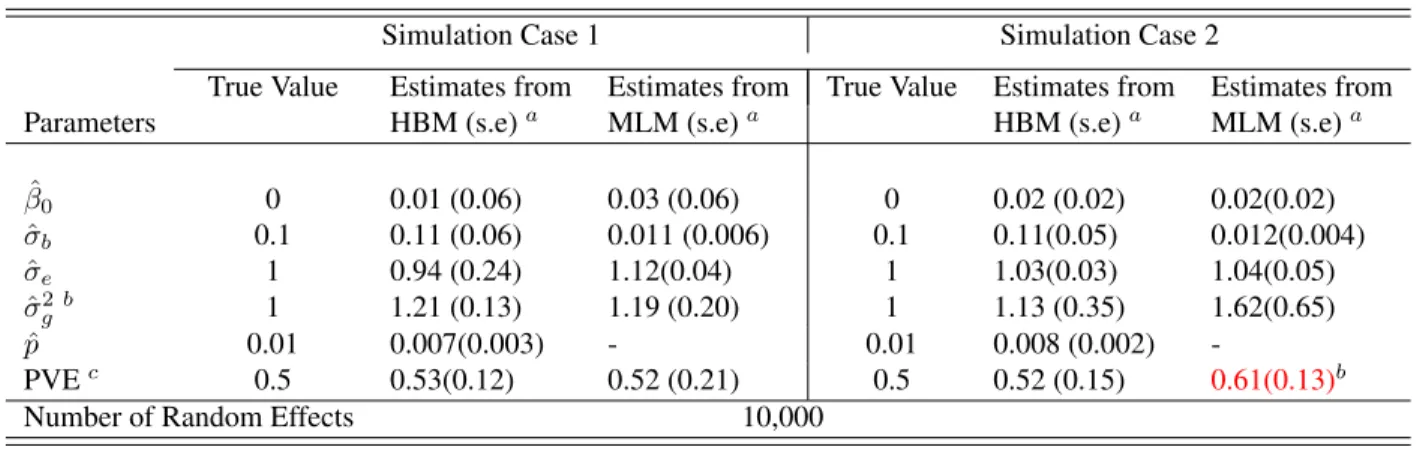
Table 2.1 shows the estimation results from the simulated data sets using the HBM and
MLM along with the true model parameters. The estimated mixture probability pˆand the
random effect variance σˆb by the HBM are close to their corresponding true values, 0.01
and 0.1, respectively. This demonstrates the good performance of our estimation method. In
both simulation cases, the MLM severely underestimates σ2
b, as it divides the total genetic
variance onto all the SNPs, instead of just the 1% association SNPs (p= 0.01), which results in underestimation of the genetic effects. In addition, in Simulation Case 2, the estimated
estimate. The reason is that the MLM can not distinguish the “significant” SNP effects
versus those “noisy” effects due to its assumption that all random effects follow the same
distribution. Therefore,σˆg2 obtained by MLM would include both “significant” and “noisy” effects and thus lead to overestimation of PVE according to (2.4). We comment that the
simulation model in this case is different from the underlying models assumed by our HBM
and the MLM of GCTA. As the results indicate, the HBM is rather robust against such model
misspecification.
Table 2.1: Example 1 - Simulation Results with number of SNPs as 10,000
Simulation Case 1 Simulation Case 2
True Value Estimates from Estimates from True Value Estimates from Estimates from
Parameters HBM (s.e)a MLM (s.e)a HBM (s.e)a MLM (s.e)a
ˆ
β0 0 0.01 (0.06) 0.03 (0.06) 0 0.02 (0.02) 0.02(0.02)
ˆ
σb 0.1 0.11 (0.06) 0.011 (0.006) 0.1 0.11(0.05) 0.012(0.004)
ˆ
σe 1 0.94 (0.24) 1.12(0.04) 1 1.03(0.03) 1.04(0.05)
ˆ σ2
gb 1 1.21 (0.13) 1.19 (0.20) 1 1.13 (0.35) 1.62(0.65)
ˆ
p 0.01 0.007(0.003) - 0.01 0.008 (0.002)
-PVEc 0.5 0.53(0.12) 0.52 (0.21) 0.5 0.52 (0.15) 0.61(0.13)b
Number of Random Effects 10,000
aValues in parenthesis are standard errors.bGenetic Varianceσˆ2
gis defined in the same way in [Yang et al., 2010a] which equals to
ˆ
σ2
b×N. N is the number of SNPs whose effectbjfollows theN(0, σ2b)distribution.cPVE is calculated as
ˆ
σ2g
(ˆσ2
g+ˆσ2e)
.
Example 2
This simulation example is used to demonstrate the performance of the HBM algorithm
when the number of SNPs is large (i.e. 100,000), in the order of real GWAS. We have to implement several computational optimizing strategies in order to speed up the computation
on such a large number of SNPs as well as to efficiently use the computer memory.
First, in each iteration of the HBM algorithm, we need to invert the covariance matrix of
posterior distribution ofb with rank as the number of SNPs: (qIq/σ2b +WITWI/σ2)
−1 .
In-stead of inverting this matrix directly, we employ the Sherman-Morrison-Woodbury formula
of observations, which usually is much smaller than the number of SNPs in genetic studies.
Secondly, computation using a large number of SNPs is intensive. Analyzing large datasets
of SNPs seems to be impractical on uniprocessor machines. Thus, we carry out the analysis
in parallel on UNC-CH’s multi-core Linux-based cluster computing server. We write scripts
to distribute the computation among multiple cores/CPUs and run multiple computing
anal-yses simultaneously. Our study shows that parallel computing can speed up the computation
by a factor of 20 on a 10-core computing node on the cluster. It takes668.5minutes and
158GB memory to finish the calculation for the simulated data set with100,000 SNPs. To consider whole genome data with even more SNPs, the amount of memory and computation
power of the server will be the main bottleneck.
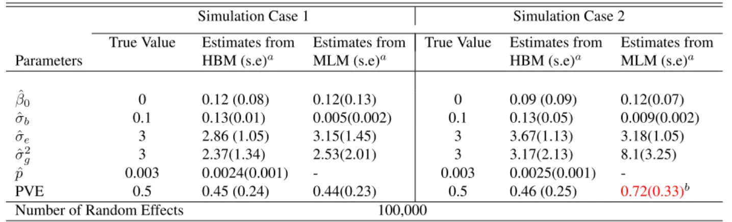
Similar to Example 1 in Section 2.3.1, we consider the same two simulation cases. The
estimation results are summarized in Table 2.2. Even for the larger number of SNPs, our
HBM still performs well in both cases, while the same drawbacks exist for the MLM.
For Example 2 (with 100,000 SNPs), Table 2.3 reports the cross table results of the
as-sociation SNPs identified by HBM against the truth. As one can see, the HBM can correctly
detect76%and82%of the true association SNPs for the two simulation cases respectively, and more than 99.9% of the true non-association SNPs. This suggests that the HBM works
very well at detecting association SNPs with the false positive rate as low as0.062% and
0.041%, respectively.
2.3.2 Real Data Set Results The Framingham Heart Study
We further apply HBM and MLM to data from the Framingham Heart Study [FHS, 2012]
to study genetic associations with the body mass index (BMI). The FHS is a
community-based, prospective, longitudinal study following three generations of participants.
Table 2.2: Example 2 - Simulation Results with Number of SNPs as 100,000
Simulation Case 1 Simulation Case 2
True Value Estimates from Estimates from True Value Estimates from Estimates from
Parameters HBM (s.e)a MLM (s.e)a HBM (s.e)a MLM (s.e)a
ˆ
β0 0 0.12 (0.08) 0.12(0.13) 0 0.09 (0.09) 0.12(0.07)
ˆ
σb 0.1 0.13(0.01) 0.005(0.002) 0.1 0.13(0.05) 0.009(0.002)
ˆ
σe 3 2.86 (1.05) 3.15(1.45) 3 3.67(1.13) 3.18(1.05)
ˆ σ2
g 3 2.37(1.34) 2.53(2.01) 3 3.17(2.13) 8.1(3.25)
ˆ
p 0.003 0.0024(0.001) - 0.003 0.0025(0.001)
-PVE 0.5 0.45 (0.24) 0.44(0.23) 0.5 0.46 (0.25) 0.72(0.33)b
Number of Random Effects 100,000
aValues in the parenthesis are standard errors.bThe PVE estimated by MLM is higher than the true values in both simulation cases.
Table 2.3: Example 2 - Detection Rate using HBM with Number of SNPs as 100,000
Association SNPs Non-association SNPs identified by HBM identified by HBM
Simulation Case 1 Association SNPs 76% 24%
Non-Association SNPs 0.062% 99.938% Simulation Case 2 Association SNPs 82% 18%
Non-Association SNPs 0.041% 99.959%
array. Genotypes on the Y chromosome are not included in our analysis. A standard quality
control filter is applied to the genotype data. Individuals with5%or more missing genotype data were excluded from analysis. SNPs that are on the X chromosomes and have a call rate
≤ 99%or a minor allele frequency≤ 0.01were also eliminated from the analysis. The ap-plication of the quality control procedures resulted in8,738individuals with287,525SNPs from the500,000genotype data. Genotype data were converted to minor allele frequencies for the analysis. One individual of a pair is deleted if the genetic relationship is greater than
0.025. Note that the genetic relationship between individualj and individualk is defined as in Yang et al. [2011a]:
Ajk =
1
N
N
X
i=1
(xij −2pi)(xik−2pi) 2pi(1−pi)
wherexij/xik is the number of copies of the reference allele for theith SNP of the jth/kth
individual andpiis the frequency of the reference allele. After the above preprocessing, there
are1,915unrelated individuals in the analysis.
Because the total number of SNPs in the FHS data is close to 300,000, computation is limited by the memory of the UNC server if we include all SNPs in the analysis. Therefore,
as a proof of concept, the13,764SNPs on Chromosome 16 are used in the analysis. Another reason for considering this chromosome is that it contains an enzyme fat mass and obesity
associated protein also known asFTO. We would like to see whether the HBM can identify
the SNPs that are significantly correlated with BMI on Chromosome 16, especially those
SNPs on theFTOgene. We include the first seven Principal Components (PCs) for BMI as
fixed effects in the model to eliminate genotype correlation induced by biological ancestry.
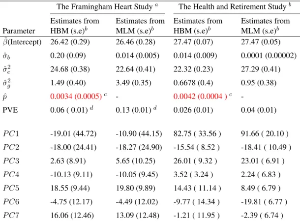
The estimation results are shown in the left panel of Table 2.4. We see that the estimated
mixture probabilitypˆfrom HBM is around 0.003, which indicates only 0.3 percent of the SNPs on Chromosome 16 are associated with BMI.
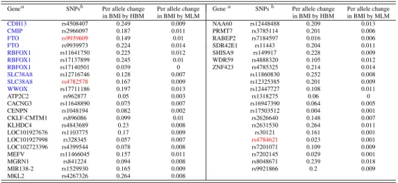
The top panel of Table 2.5 lists the 43 SNPs that are identified by HBM as
associ-ated with BMI, which are ordered according to their names, along with the
correspond-ing genes if available. Among these identified SNPs, the SNP rs9939609 variant has been
found to be associated with obesity risk among children and adolescents of Beijing, China
by Xi et al. [2010], and with BMI and waist circumference among European- and
African-American youth by Liu et al. [2010]. The SNP rs9939973 on the FTOgene has also been
found to be related with overweight of children in Korea by Lee et al. [2010a]. These
two SNPs are in strong linkage disequilibrium (LD) with SNP rs1558902 (Rsq=0.901 for
rs9939609 and Rsq=0.905 for rs9939973), which had been previously reported in a
well-known GWAS [Speliotes et al., 2010]. The detection results can also be replicated to some
extent: the three SNPs highlighted in red and the genes indicated in blue are also detected in
Table 2.4: Real Data Estimation Results using HBM and MLM
The Framingham Heart Studya The Health and Retirement Studyb Estimates from Estimates from Estimates from Estimates from Parameter HBM (s.e)b MLM (s.e)b HBM (s.e)b MLM (s.e)b
ˆ
β(Intercept) 26.42 (0.29) 26.46 (0.28) 27.47 (0.07) 27.47 (0.05)
ˆ
σb 0.20 (0.09) 0.014 (0.005) 0.014 (0.009) 0.0001 (0.00002)
ˆ
σ2e 24.68 (0.38) 22.64 (0.41) 22.32 (0.23) 27.29 (0.41)
ˆ
σ2
g 1.49 (0.40) 3.49 (0.35) 0.6678 (0.4) 0.95 (0.38)
ˆ
p 0.0034 (0.0005)c - 0.0042 (0.0004 )c
-PVE 0.06 ( 0.01)d 0.13 (0.01)d 0.026 (0.01) 0.04 (0.01)
P C1 -19.01 (44.72) -10.90 (44.15) 82.75 ( 33.56 ) 91.66 ( 20.10 )
P C2 -18.00 (24.41) -18.27 (24.90) -15.54 ( 8.52 ) -18.41 ( 10.49 )
P C3 2.63 (8.91) 5.65 (10.25) 26.01 ( 9.32 ) 23.01 ( 6.91 )
P C4 -10.13 (9.11) -10.05 (9.45) 3.52 ( 3.24 ) 2.24 ( 6.83 )
P C5 18.55 (9.44) 19.80 (9.89) 14.43 ( 11.14 ) 8.49 ( 6.79 )
P C6 -4.75 (12.17) -4.49 (12.02) -9.77 ( 14.34 ) -19.81 ( 6.77 )
P C7 16.06 (12.46) 13.09 (12.48) -1.21 ( 11.95 ) -2.39 ( 6.74 )
aThe analysis is based on1,915unrelated persons in the Framingham Heart data set using13,764SNPs on
Chromosome 16 to predict BMI.bThe analysis is based on12,237unrelated persons in the Health and Retirement
Study using11,925SNPs on Chromosome 16 to predict BMI.cValues in the parenthesis are standard errors.d
PVE estimated by MLM is higher than that estimated by HBM.
The predicted allele effects on BMI (kg/m2per allele) by HBM and MLM are compared
in Table 2.5, which are calculated as the posterior mean of the random effects under each
model. The allele effect predicted by HBM is closer to the findings in the previous GWAS.
As an example, we compare SNP rs9939973’s effect on BMI with rs1558902’s, both of
which are on theFTOgene and are highly correlated. Speliotes et al. [2010] found that the per allele change in BMI for SNP rs1558902 is 0.39 (kg/m2) based on a total of 249,796 individuals of European ancestry using a GWAS method. It is much closer to the estimate
obtained by HBM (0.224kg/m2), rather than the much-lower estimate given by MLM (0.014
kg/m2). This comparison indicates that the MLM, assuming that every SNP has an effect on
One can also see from Table 2.4 that the estimated PVEs are different (5.6%vs. 13.3%). In Section 2.3.1, we have shown that the MLM tends to overestimate PVE if there exist many
SNPs with small/noisy effects on the phenotype, which we think is also the case for the FHS
data here. To demonstrate that there exist SNPs with small effects on BMI, we perform
the following multi-scale analysis by varying the amount of SNPs on Chromosome 16 to
be included in MLM and showing how the corresponding estimated PVE changes. We first
regress BMI on every single SNP and obtain the correspondingp-value. Then we consider
a range of varying thresholds on the p-values, and only include those SNPs with ap-value
below the threshold in the MLM when estimating the PVE. We systematically increase the
p-value threshold so that more and more SNPs that are “less” significant will be included.
The idea is that as the p-value threshold increases, more SNPs with small effects on BMI will
be included when estimating PVE, which will result in higher PVEs. The estimation results
are presented in Table 2.6. The estimated PVE decreases from18% to1% as a decreasing
number of SNPs with smallerp-values (below the thresholds from10−1to10−7) are included in the analysis. The results indicate that when estimating PVE using MLM, the more SNPs
with small effects on BMI are included, the higher the estimated PVE is.
In summary, the analysis of the Framingham data reveals several important empirical
findings: (1) Among all the SNPs on Chromosome 16, only0.003of them are significantly associated with BMI according to HBM; (2) Several association SNPs identified by HBM
have also been reported to be significantly related with BMI in previous studies; (3) The
MLM tends to underestimate the allele effect on the phenotype while the HBM estimates
much closer to previous GWA study results; (4) Because the MLM includes SNPs with small
The Health and Retirement Study
In this section, we try to replicate the results in Section 2.3.2 using data from the Health
and Retirement Study [HRS, 2012]. The HRS is a longitudinal study of Americans over
age 50, conducted every two years from 1992 to 2012; it collects information on economic,
health, social, and other factors relevant to aging and retirement. DNA samples were
col-lected in 2006 and 2008. Out of the colcol-lected samples, 13,129 individuals were put into genotyping production and12,507passed the University of Washington Genetics Coordinat-ing Center’s standardized quality control process.
The HRS analysis was performed on12,237unrelated individuals and the11,925SNPs on Chromosome 16 that are common to those SNPs used in the FHS analysis of Section 2.3.2.
The estimation results are shown in the right panel of Table 2.4 and Table 2.5. We first
note that the HBM estimates of the proportion of association SNPs are very close in the two
studies:0.34%and0.42%for FHS and HRS respectively. Both data sets identified the same set of six genes for BMI including the well-knownFTOgene. These genes account for about
25%of the genes identified in our analysis.
Forty SNPs are identified to be associated with BMI by the HBM using HRS data set,
which are listed in the bottom panel of Table 2.5. Between the two studies, the HBM
iden-tifies three common SNPs to be associated with BMI: rs4782578, rs4784621 and rs9939606
(shown in red), as well as a few common genes (shown in blue). Furthermore, SNP rs9940128
identified using the HRS data is also on theFTOgene, and has been found before to be cor-related with BMI by Hotta et al. [2008], Tan et al. [2008] and Ramya et al. [2011].
2.4 Conclusion
In this paper, we propose a Hierarchical Bayesian Model (HBM) that extends the MLM
of Yang et al. [2011a]. Our model allows SNP effects on phenotypes of interest to follow a
Table 2.5: Per Allele Change in BMI for Association SNPs Identified by HBM
The Framingham Heart Study
Genea SNPsb Per allele change Per allele change Genea SNPsb Per allele change Per allele change
in BMI by HBM in BMI by MLM in BMI by HBM in BMI by MLM
CDH13 rs4508407 0.249 0.009 NAA60 rs12448488 0.209 0.013
CMIP rs2966097 0.187 0.011 PRMT7 rs3785114 0.201 0.006
FTO rs9939609 0.149 0.01 RABEP2 rs7184597 0.016 0.006
FTO rs9939973 0.224 0.014 SDR42E1 rs11443 0.204 0.011
RBFOX1 rs11641750 0.225 0.012 SHISA9 rs149917 0.228 0.009
RBFOX1 rs17137899 0.245 0.01 WDR59 rs4888320 0.105 0.012
RBFOX1 rs17140501 0.039 0 ZNF423 rs4785325 0.214 0.014
SLC38A8 rs12716746 0.128 0.007 rs11860830 0.252 0.008
SLC38A8 rs4782578 0.167 0.009 rs12325385 0.201 0.009
WWOX rs17711186 0.197 0.013 rs12447727 0.108 0.011
ATP2C2 rs962877 0.05 0.003 rs1318275 0.06 0
CACNG3 rs11648890 0.075 0.007 rs16947390 0.064 0.005
CENPN rs1048194 0.082 0.002 rs17503512 0.004 0.001
CKLF-CMTM1 rs896086 0.099 0.01 rs2626640 0.148 0.007
KLHDC4 rs4843689 0.23 0.008 rs2631530 0.264 0.011
LOC101927676 rs1103775 0.17 0.009 rs30121 0.161 0.001
LOC101927998 rs328345 0.057 0.007 rs4784621 0.023 0.001
LOC102723396 rs4399544 0.078 0.008 rs7201071 0.109 0.009
MEFV rs11466045 0.157 0.011 rs7202145 0.029 0.001
MGRN1 rs841224 0.094 0.008 rs8048671 0.239 0.018
MIR138-2 rs1529930 0.165 0.009 rs9921866 0.2 0.009
MKL2 rs4267326 0.264 0.008
The Health and Retirement Study
Genea SNPsb Per allele change Per allele change Genea SNPsb Per allele change Per allele change
in BMI by HBM in BMI by MLM in BMI by HBM in BMI by MLM
CDH13 rs7199677 0.14 0.005 KIAA0513 rs8045387 0.112 0.001
CMIP rs10514518 0.123 0.002 LOC102724927 rs2601773 0.112 0.002
FTO rs9939609 0.143 0.003 MPHOSPH6 rs2303267 0.183 0.007
FTO rs9940128 0.163 0.009 NDRG4 rs11076243 0.133 0.002
RBFOX1 rs11076998 0.162 0.004 PAPD5 rs7191151 0.129 0.003
RBFOX1 rs11647425 0.104 0.001 PSKH1 rs2136648 0.141 0.005
RBFOX1 rs12448747 0.173 0.004 RP11-488I20.3 rs13332284 0.202 0.011
RBFOX1 rs1473145 0.132 0.003 URAHP rs9921920 0.121 0.008
RBFOX1 rs17562548 0.211 0.02 VAT1L rs13330130 0.11 0.001
RBFOX1 rs1860304 0.174 0.006 rs11075417 0.147 0.003
SLC38A8 rs4782578 0.137 0.009 rs1362441 0.122 0.002
WWOX rs16948787 0.111 0.004 rs154554 0.16 0.002
WWOX rs4888855 0.223 0.019 rs16960867 0.151 0.005
BCAR1 rs4261573 0.118 0.001 rs4023915 0.155 0.006
CDH11 rs1520229 0.183 0.009 rs4467088 0.113 0.002
CLEC16A rs767019 0.115 0.002 rs4784621 0.106 0.001
CMC2 rs2549855 0.111 0.002 rs7187990 0.104 0
CNGB1 rs7184838 0.172 0.012 rs8045580 0.126 0.005
CNTNAP4 rs4888514 0.178 0.008 rs964933 0.114 0.001
GPR139 rs868554 0.14 0.002 rs9925215 0.119 0.005
aThe same genes are identified associated with BMI using both FHS and HRS data are shown in blue.bSNPs
identified to be associated with BMI in both FHS and HRS data are shown in red.
the challenge of high-dimensionality in GWAS data by incorporating simultaneous selection
of genetics variables that are jointly significant in predicting the phenotype. We employ
several computing tricks that enable us to analyze a large number of SNPs (in the order of
100,000).
We demonstrate the applicability of our approach using both simulated and real data. The
Table 2.6: The Framingham Heart Study: PVE Estimation Using Proportion of SNPs Based on P-value Thresholda
P-value<0.1b c P-value<0.01b c P-value<0.001b c P-value<0.0001b c
(s.e.) (s.e.) (s.e.) (s.e.)
Number of SNPs 2690 561 145 45
Genetic Variance 4.45 (0.34) 3.34 (0.37) 2.08 (0.38) 0.86 (0.31)
Error Variance 20.66 (0.34) 22.31 (0.35) 24.06 (0.38) 25.25 (0.39)
Total Variance 25.11 (0.45) 25.65 (0.50) 26.14 (0.53) 26.11 (0.50)
PVE 0.18d(0.06) 0.13d(0.04) 0.08d(0.03) 0.03d(0.01)
P-value<0.00001b c P-value<0.000001b c P-value<0.0000001b c
(s.e.) (s.e.) (s.e.)
Number of SNPs 21 10 7
Genetic Variance 0.43 (0.21) 0.43 (0.28) 0.25 (0.22)
Error Variance 25.48 (0.40) 25.60 (0.40) 25.73 (0.40)
Total Variance 25.91 (0.45) 26.03 (0.49) 25.97 (0.46)
PVE 0.02d(0.01) 0.02d(0.01) 0.01d(0.01)
aThe analysis in the table is carried out using the GCTA software developed by Yang
et al. [2011a].bP-value is obtained by regressing BMI on each single SNP.cValues in the
parenthesis are standard errors. dPVE decreases from18%to1%as a smaller group of
SNPs are included in the analysis.
We then analyze real data from the FHS and the HRS to identify SNPs on Chromosome
16 that are associated with the body mass index (BMI). The identified SNPs are consistent
with earlier findings in the literature, and the results can be replicated across the two studies.
The results from both the simulations and the real applications suggest that the MLM tends
to over-estimate the proportion of total genetic variance over total phenotypic variance, i.e.
PVE. The reason is that the MLM assumes that all the SNPs have effect on the phenotype,
including those SNPs with small or noisy effects.
Our work offers a flexible framework that can be extended in several aspects. We now
of-fer some discussion regarding potential future work directions. To analyze the whole-genome
data, we can follow Lee et al. [2008] and Yang et al. [2011c] to analyze each chromosome
separately. We believe that more work is needed to rigorously study how to aggregate the
results, and leave that for future work. The current assumption on the mixture distribution,
i.e. a point mass at zero plus a normal distribution, may not be flexible enough to capture
genetic effects in certain situations. We intend to relax the distributional assumption to a
mixture of a point mass at zero plus a nonparametric distribution as in Lee et al. [2014]. One
challenge is that the computational short cut we used in this study for Gibbs Sampling might
not remain effective for more flexible distributions; hence alternative algorithms have to be
potential dependence among SNPs within LD blocks. One difficulty then is the estimation
of (potentially arbitrary) correlation structure among the SNPs. We are experimenting with
adapting the principal factor approximation idea of Fan et al. [2012a] into our current
Table 2.7: The HBM Algorithm
Initialize
Choose starting values of[β(0), b(0), I(0), p(0), σ2
e
(0)
, σ2
b
(0)
].
Iterate
1. Drawβ(t)fromP(β(t)|Y, b(t−1), σ2
b
(t−1)
, σ2
e
(t−1)
).
P(β|Y, b, σ2
b, σe2)∝exp{−
1 2σ2
e(y−Xβ−W b)
t(y−Xβ−W b)}exp{−1 2β
tΣ−1
k β},
whereΣkis ak×k matrix withσa2on the main diagonal and0everywhere else, with
kbeing the dimension ofβ.
2. Drawb(t)fromP(b(t)|Y, β(t−1), I(t−1)
j = 1, σ2b
(t−1)
, σ2
e
(t−1)
)andbj is set to zero if
Ij(t−1) = 0.
P(b|Y, β, Ij = 1, σb2, σ2e)∝
exp{− 1
2σ2
e(y−Xβ−WIb)
t(y−Xβ−W
Ib)} ×exp{−12bt(Dq−2)b}, whereWIare
the columns ofW corresponding toIj(t−1) = 1, andDis the diagonal matrix with the main diagonal asσ2b and the dimension asq =P
j(I
(t−1)
j = 1)
3. DrawIj(t) fromP(Ij(t)|Y, β(t), b(t)
j , σb2
(t−1)
, σ2
e
(t−1)
).
P(Ij|Y, β, bj, σb2, σ2e) =
p×φ(bj,σb)
p×φ(bj,σb)+(1−p)×φ(bj,σ), whereφstands for the standard
normal density.
4. Drawp(t)fromP(p(t)|Y, β(t), I(t), b(t), σ2
b
(t−1)
, σ2
e
(t−1)
).
P(p|Y, β, I, b, σ2
b, σ2e)∝p
Pq
j=1Ij(1−p)q−PIq=1Ijpα0−1(1−p)β0−1
5. Drawσ2
e
(t)
fromP(σ2
e
(t)
|Y, β(t), I(t), b(t), σ2
b
(t−1)
).
P(σ2
e|Y, β, I, b, σb2)∝(σe2)
−n/2exp(−(y−Xβ−W b)t(y−Xβ−W b)
2σ2
e )(σ
2
e)
−a1−1exp(−b2 1 σ2
e ).
6. Drawσ2
b
(t)
fromP(σ2
b
(t)
|Y, β(t), I(t), b(t), σ2
e
(t)
).
P(σb2|Y, β, I, b, σe2)∝(σb2)−
P
1Ij=1/2
exp(−
P
1Ij=1(bj)2
2σ2
b
)(σb2)−a2−1exp(−b22 σ2
b
CHAPTER 3: LEAST SQUARES SIEVE ESTIMATION OF MIXTURE DISTRIBUTIONS WITH BOUNDARY EFFECTS
3.1 Introduction
In this paper, we consider measurement error models where we observe only the
error-contaminated variableY =X+Z, whereXis the unobservable random variable of interest, andZ is the measurement error with a known densityfz that is independent ofX. We are
interested in estimating the distribution of X, which is assumed to be a mixture of several
point masses and a continuous distribution. We are particularly interested in the case that the
continuous part is supported on a finite interval, and has non-smooth boundaries.
Distribution estimation in measurement error models has been widely studied, but most
of the earlier studies focused on estimating continuous density functions. Recently there are
two studies (Van Es et al. [2008] and Lee et al. [2010b]) which consider mixtures of one
discrete atom and one continuous component in the context of measurement error models,
and independently propose the same estimator. The convergence rate of the estimator is
recently derived by Gugushvili et al. [2011].
In terms of purely continuous distributions, there are two major types of deconvolution
approaches. The first type uses ideas of Fourier and inverse Fourier transformation along with
nonparametric smoothing. Examples of this approach are the papers by Van Es et al. [2008],
Lee et al. [2010b] and references therein. The second type includes non-Fourier based
decon-volution methods. In this group, many studies first employ basis functions such as B-splines
or wavelets to expand the target density (or distribution) function, and then estimate the basis
Stauden-mayer et al. [2008] and references therein. In addition, several alternatives for deconvolution
have been proposed, such as NPMLE, SIMEX, and TAYLEX, which are well reviewed in
Carroll et al. [2006], Wagner and Stadtm¨uller [2008], and Wang et al. [2009].
Compared with the other studies, Lee et al. [2013] covers more general cases of
mea-surement error models that have two features: 1) discrete and continuous mixtures, and 2)
non-smooth boundaries. First they approximate the distribution of X using discretization,
which gives a sieve of the distribution family. Then they estimate the distribution using
maximum likelihood (ML) within each sieve. Sieve type estimators have been proposed for
deconvolution problems by Cordy and Thomas [1997] where degenerate distributions are
used to approximate the continuous mixture component. In the error-free case, Ruppert et al.
[2007] proposed a sieve type density estimator for certain special distributions with known
boundaries.
However, the ML method of Lee et al. [2013] involves long computation time and is
not robust against a misspecified error distribution. In this study, we propose alternative least
squares (LS) sieve estimators based on the cumulative distribution function and characteristic
function, instead of maximum likelihood. Our simulation results clearly demonstrate the
advantages of the LS estimators. First, computational cost is much smaller when using the LS
method. For example, it takes 113.32 seconds for the ML method on a simulated data set with
sample size of 329, while it only takes 0.30 second using the cumulative distribution function
based LS estimator. Secondly, in Section 3.4.1 the LS estimators are seen to give smaller
(integrated) mean squared error. Furthermore, as seen in Section 3.4.2, the LS estimators are
more robust when the error distribution is misspecified.
The remainder of the paper is organized as follows. Section 3.2 explicitly describes our
model, and then proposes the two LS-sieve estimators, along with their estimation
algo-rithms. In Section 3.3, consistency of the proposed estimators is established under
methods via simulation studies, and compares the ML-sieve with the LS-sieve estimators.
Section 3.5 contains an application to the Framingham Heart Study data. Our methods are
used to identify the distribution of some important SNPs’ effects on body mass index (BMI).
We conclude the paper in Section 3.6 with discussion of future work. Technical proofs are
provided in the Appendix.
3.2 The Model and The Estimators
3.2.1 The Model
Suppose that we can only observe an error contaminated variableY, instead ofXwhose
distribution is a mixture of several point masses plus a continuous distribution. That is,
Y =X+Z, (3.8)
whereZ is a measurement error with known densityfZ, and is independent ofX. Our goal
is to use a random sampleY1, ...,Ynto estimatefX, the generalized density ofX, which is a
mixture of discrete point massesal,l = 1, . . . , ν, and a continuous random variableXcwith
densityfc, using weightsπ1,...,πν, and πν+1. Hence, the generalized densityfX(x)has the
following form:
fX(x) = ν
X
l=1
πlδal(x) +πν+1fc(x), (3.9)
whereδal is the Dirac delta function atal. Here, the weights are probabilities in the sense
that eachπl is nonnegative,Pνl=1+1πl = 1. We are particularly interested in the case wherefc
is supported on a finite interval[a, b]. This paper focuses on scenarios where the valuesνand
a1, ..., aν are known. In this setting, the estimation offX is equivalent to the estimation of
can be extended to cases where the locations of the pointmass are unknown, which we will
discuss in Section 3.6.
The first step is discretization of the continuous variable Xc. We approximateXc by a
discrete random variableX˜c taking values on an equally spaced grid, with grid spacing h.
The discrete variable X˜c takes on values xj :xj+1−xj =h, j = 1, ..., r, which cover the
support offc. In practice, we chooseX˜csatisfying
˜
Xc=xj if and only if Xc∈[xj −0.5h, xj + 0.5h).
The parameterhplays a role similar to the bin width in histogram estimation, and the same as
the smoothing parameter in kernel density estimation. Letθ = (θ1, ..., θr)T be the probability
distribution ofX˜c, i.e.
θj =P( ˜Xc =xj) for each j = 1, ..., r,
whereθj ≥ 0and
P
θj = 1. Then eachθj approximates the probability thatXclies in the
interval[xj −0.5h, xj + 0.5h).
When we replaceXcby X˜c, the corresponding distribution of X is purely discrete, and
the generalized densityfX can be approximated as
˜
fX(x|π, θ) = ν
X
l=1
πlδal(x) +πν+1
r
X
j=1
θjδxj(x). (3.10)
Based on this approximation, our problem turns into the problem of estimatingθandπ. Lee
et al. [2013] used maximum likelihood to estimate these parameters. Below, we propose two
3.2.2 LS Based on Cumulative Distribution Functions
The first approach is based on cumulative distribution functions (cdf). A natural idea is to
minimize the distance between the true distribution ofY and the approximated distribution
function, which has the form
˜
FY(y|π, θ) = ν
X
l=1
πlFZ(y−al) +πν+1
r
X
j=1
θjFz(y−xj), (3.11)
where FZ is the distribution function of Z. This approach is reasonable, but a problem is
that the true distribution ofY is unknown. As an alternative, we use the empirical
distribu-tion funcdistribu-tion. A justificadistribu-tion is that the empirical distribudistribu-tion funcdistribu-tion converges to the true
distribution as the sample size goes to infinity.
Hence we estimateθandπby minimizing the (weighted) distance between two
distribu-tion funcdistribu-tions, i.e.
(ˆπ,θˆ) = arg min
π,θ Scdf(π, θ) = arg minπ,θ
Z
|Fˆn(y)−F˜Y(y|π, θ)|2w(y)dy (3.12)
whereFˆn(y) = 1/nPkI(Yk ≤ y) is the empirical distribution, andw(·) is a nonnegative
weight function satisfyingR w(y)dy= 1. In this study, we use uniform weight on support of
yasw(y).
Note thatScdf(·,·)is a quadratic function of bothθ andπ. In addition, these parameters
are defined on compact subsets of the Euclidean space. Hence there exists a unique minimizer
of (3.11). A problem is that the minimizer does not have a closed form because of the
constraints onθandπ. We use an iterative minimization algorithm to compute the minimizer.
Details on the estimation algorithm are given in the Appendix.
as
˜
fX(x|ˆπ,θˆ) = ν
X
l=1
ˆ
πlδal(x) + ˆπν+1
r
X
j=1
ˆ
θjδxj(x). (3.13)
We can improve the above estimator by using a linear interpolation such as
˜
fX(x|π,ˆ θˆ) = ν
X
l=1
ˆ
πlδal(x) + ˆπν+1
r
X
j=1
ˆ
θjfˆc(x|θˆ), (3.14)
where
ˆ
fc(x|θˆ) =
ˆ
θj−1 h +
ˆ
θj−θˆj−1
h(xj−xj−1)(x−xj), forx∈[xj−1, xj),1≤j ≤r+ 1;
0, otherwise,
(3.15)
which is a linear interpolation of the(xj,θˆj)s. Here, we usex0 =x1−0.5h,xr+1 =xr+0.5h, ˆ
θ0 = ˆθ1 andθˆr+1 = ˆθr. The estimator in (3.14) is attractive especially whenfcis known to
be continuous because the estimator offcis also a continuous density.
3.2.3 LS Based on Characteristic Functions
An alternative is to base the estimation on characteristic functions instead of cumulative
distribution functions. The convergence theorem 6.3.3 of Chung [2001] proved that
conver-gence of characteristic functions implies the converconver-gence of the corresponding distribution.
In addition, the empirical characteristic function converges to the true function as the size of
a random sample goes to infinity. Hence we expect that the distance between the empirical
characteristic function and the characteristic function corresponding to (3.11) might be small
if the parameters are well estimated. From that, we estimateθandπas the minimizers:
(ˆπ,θˆ) = arg min
π,θ Schf(π, θ) = arg minπ,θ
Z