Contents lists available atScienceDirect
Physica A
journal homepage:www.elsevier.com/locate/physa
Scaling of global input–output networks
Sai Liang
a, Zhengling Qi
b,c, Shen Qu
a, Ji Zhu
b, Anthony S.F. Chiu
d,
Xiaoping Jia
e, Ming Xu
a,f,∗aSchool of Natural Resources and Environment, University of Michigan, Ann Arbor, MI 48109-1041, United States bDepartment of Statistics, University of Michigan, Ann Arbor, MI 48109-1107, United States
cDepartment of Statistics and Operations Research, University of North Carolina, Chapel Hill, NC 27599-3260, United States dDepartment of Industrial Engineering, De La Salle University, Manila 1004, Philippines
eSchool of Environmental and Safety Engineering, Qingdao University of Science & Technology, Qingdao 266042, China fDepartment of Civil and Environmental Engineering, University of Michigan, Ann Arbor, MI 48109-2125, United States
h i g h l i g h t s
• Four distributions can better describe scaling patterns of input–output networks.
• Global input–output networks do not follow power law distributions.
• Dataset choice has limited impacts on the observed scaling patterns.
a r t i c l e i n f o
Article history:
Received 8 April 2015
Received in revised form 17 November 2015
Available online 15 February 2016
Keywords:
Economic network Input–output table Scaling
Macroeconomics
a b s t r a c t
Examining scaling patterns of networks can help understand how structural features relate to the behavior of the networks. Input–output networks consist of industries as nodes and inter-industrial exchanges of products as links. Previous studies consider limited measures for node strengths and link weights, and also ignore the impact of dataset choice. We con-sider a comprehensive set of indicators in this study that are important in economic anal-ysis, and also examine the impact of dataset choice, by studying input–output networks in individual countries and the entire world. Results show that Burr, Log-Logistic, Log-normal, and Weibull distributions can better describe scaling patterns of global input–output net-works. We also find that dataset choice has limited impacts on the observed scaling pat-terns. Our findings can help examine the quality of economic statistics, estimate missing data in economic statistics, and identify key nodes and links in input–output networks to support economic policymaking.
©2016 Elsevier B.V. All rights reserved.
1. Introduction
An economy comprises industrial activities (called industries in this study) exchanging goods and services with each other. An industry (or sector) uses products from other industries as inputs to produce products consumed by other industries and final consumers (e.g., households and government), as described by the System of National Accounts (SNA) [1]. In a real-world economy, an industry may be densely connected through the exchange of products with particular industries,
∗Correspondence to: University of Michigan, Ann Arbor School of Natural Resources and Environment, 440 Church Street, 3006 Dana Building, Ann
Arbor, MI 48109-1041, United States. Tel.: +1 734 763 8644; fax: +1 734 936 2195.
power grid [14], brain functional networks [17], neuronal avalanches [18], and social networks [19]. Specifically, several studies examined scaling patterns of IO networks in order to identify common structural features shared across economies. McNerney et al. [7] found that link weights measured by intermediate economic flows of individual countries follow the Weibull distribution, and node strengths measured by industrial economic outputs follow the exponential distribution. Cerina et al. [6] found that the weights of links in the global economy follow the Log-normal distribution. Despite these limited studies, there are still three research gaps to be filled.
First, previous studies use intermediate flows (i.e., the value of exchanged products between industries in a given year) to measure the weights of links [6,7]. Industrial interdependence of an IO network, however, can be more than just the direct exchanges of products [2–4]. For example, a supply chain between two nodes shows a path starting from one node, passing through certain intermediate nodes, and ending at the other node. Thus, two nodes of an IO network are interdependent through not only directly exchanged products but also supply chains. Such supply chain-based interdependence is equally important to economic analysis as direct exchanges of products.
Second, existing studies use industrial total outputs to measure nodes of an IO network [7]. There are other indicators popularly used in economic studies to measure nodes (e.g., industrial final demands and value added) [13]. Using those indicators as node strengths can potentially reveal additional insights on the structure of IO networks.
Third, different datasets have different region and industry resolutions (i.e., the number of regions and industries an economy is divided into) which can significantly impact the results of some economic analyses [20,21]. It is not clear whether the structure of IO networks depends on dataset choice or not. In theory, we want to identify structural properties that are shared by IO networks across a wide range of datasets.
This study addresses these research gaps on three fronts. First, we use additional commonly used indicators to measure node strengths (i.e., industrial total outputs, industrial final demands, and industrial value added) and link weights (i.e., direct requirement coefficients, total requirement coefficients, and intermediate inter-industrial flows). Second, we examine the scaling of the global IO network at both the individual country scale and the global scale. Third, we test whether dataset choice impacts the scaling of the global IO network.
2. Methods and data
2.1. Input–output (IO) networks
IO data describe an economy as a set of industries (i.e., nodes in IO networks) connected by inter-industrial product flows (i.e., links in IO networks) [13,22–24].Fig. 1uses a three-industry example to illustrate product flows among industries within an economy. An industry uses products from other industries for its production, and then provides its products to satisfy final demand and the production of other industries. Value added is created during the production of this industry. Final demand means the amount of products being directly consumed by final users (i.e., household consumption, government expenditure, fixed capital formation, inventory changes, and exports). Value added is the net additions to the wealth of an economy (i.e., employee compensation, depreciation of fixed assets, net tax on production, and net operating surplus).
Product flows among industries inFig. 1are named intermediate flows. Intermediate flows of an industry includes its intermediate inputs (i.e., product inputs from itself and other industries) and its intermediate outputs (i.e., products allocated to the production of itself and other industries).
For a particular industry, the sum of its intermediate outputs and final demand equals to its total output, and the sum of its intermediate inputs and value added equals to its total input. Moreover, an industry’s total output equals to its total input.
We can get a matrixArepresentingdirect requirement coefficients[13] based on industrial total outputs (defined as the output vectorxrepresenting the total output of each industry) and intermediate flows (defined as the direct requirement matrixZrepresenting product flows among industries), as shown in Eq.(1).
Fig. 1. Product flows among industries within a three-industry economy. Taking industry 2 for example,z12means product flow from industry 1 to industry 2,z22means product flow from industry 2 to itself, andz21means product flow from industry 2 to industry 1. The notationv2means value added created by industry 2 which are primary inputs (e.g., labors and capital) for the production of industry 2, andy2means final demand of product from industry 2.
The elementaijin matrixArepresents direct product flow from industryito produce unitary total output in industryj. The hat
ˆ
onxmeans diagonalizing the vectorx.We can express total outputsxas a function of final demandsyby
x
=
(
I−
A)
−1y (2)whereyis the final demand vector representing final demand of products produced by each industry.
The matrix
(
I−
A)
−1is calledtotal requirement coefficientsorLeontief Inversematrix [13], elementlijin which represents both direct and indirect inputs from industryito produce one unit of finally consumed products in industryj.Iis the identity matrix. Total requirement coefficients between two industries represent the dependence of one industry on another throughout the entire supply chains.We use three indicators including industrial total outputs (i.e., total output vectorx), industrial final demands (i.e., final demand vectory), and industrial value added (i.e., value added vector
v
) to measure node strengths. Three indicators including intermediate flows (i.e., direct requirement matrixZ), direct requirement coefficients (i.e., direct requirement coefficient matrixA), and total requirement coefficients (i.e., total requirement coefficient matrixL) are used to measure link weights. Distributions of these six indicators are fitted against various distribution functions, such asPower Lawdistributions [16,25–27], Log-normal distribution [6,7], and Weibull distribution [7,28]. We consider 18 types of distribution functions in total (listed in the Supporting Information (SI)) in this study to cover a wide range of possible scaling patterns. We first calculate the frequency of each data, and then fit data values and their frequencies against various distributions.
2.2. Data sources
We use three databases in this study: the STAN Input–Output Database from the Organisation for Economic Co-operation and Development (OECD, 2006 edition) [29], the World Input–Output Database (WIOD, released in November 2013) [30,31], and the Eora database (versions v199.82 and v199.324) [32]. We use the OECD and WIOD databases for distribution fitting, and compares distribution fitting based on the Eora database with that based on the WIOD to examine the impact of dataset choice on scaling patterns. The OECD database includes only domestic IO data for isolated individual countries, while the WIOD and Eora databases provide IO data for the entire world. In particular, Eora v199.82 (Eora-original) describes each country by the original industry classifications from government statistics, while Eora v199.324 (Eora-26) aggregate the data to a unified 26-industry format (i.e., every country has the same 26 industries).
For OECD data, we use basic-price industry-by-industry IO data for domestic economic transactions of 29 individual countries. Each country is divided into 48 industries (Table S1). These IO tables are generally for the years of 1995, 2000, and 2005, with minor variations for several countries (Table S2). We convert all current-price IO data using the 2005 constant price by price indexes from OECD and World Bank databases [33,34] in order to make time-series IO data comparable. For the power law distribution fitting, because IO data for different countries are in different currencies, we convert all IO data using US Dollars (USD) by exchange rates also from OECD [35]. We use exchange rates instead of purchasing power parity in order to be consistent with compilation methods of the WIOD database [30,31].
For WIOD data, we use basic-price industry-by-industry IO data for the world economy from 1995 to 2009. WIOD covers 40 major countries/regions (i.e., 27 European Union countries and 13 other major countries/regions in the world) and the Rest of the World (RoW). Each country/region is uniformly divided into 35 industries (Table S3). Thus, WIOD data for one year include product exchanges between 1435 industries in 41 countries/regions in the world. We convert 15 sets of current-price IO data from 1995 to 2009 using the 1995 constant current-price by current-price indexes also from WIOD [30,31].
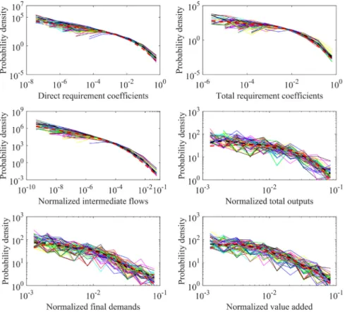
Fig. 2. Probability density distribution fits of pooled economic data for 29 individual countries from the OECD database. The black dashed line represents the pooled data, and the red dashed line represents the best-fit distribution to the pooled data. Each solid line represents a country. Intermediate flows and industrial total outputs are normalized by total through-flow of the economy which is the sum of all industrial total outputs. Industrial final demands are normalized by the sum of all industrial final demands representing total final demand of the economy. Industrial value added is normalized by the sum of all industrial value added representing gross domestic products (GDP) of the economy. As the OECD data have fewer number of links and nodes which may not be sufficient enough for deriving probability density distributions, we also plot cumulative distributions for better illustration, as shown in Figure S3. (For interpretation of the references to color in this figure legend, the reader is referred to the web version of this article.)
and Eora data are significantly different from each other in terms of country and industry resolutions. WIOD divides the world economy into 1435 industries in 41 countries/regions [30,31], while Eora-original and Eora-26 have 9812 industries in 190 countries/regions and 4873 industries in 187 countries/regions, respectively [21,32]. Note that the original Eora data are in the format of Supply-Use Tables (SUTs), instead of the industry-by-industry format used by OECD and WIOD data. We convert SUTs into the industry-by-industry format for Eora-original and Eora-26 according to methods of Miller and Blair [13]. Details on the conversion processes are shown in the SI.
3. Results
3.1. Distribution fitting
We calculate probability densities of node strengths and link weights. We then fit these probability densities with particular distributions according to log-likelihood. Higher log-likelihood value indicates better fit [7]. Fig. 2 shows probability density distribution fits of pooled IO data for 29 individual countries from the OECD database. Probability density distributions of node strengths and link weights are heavy-tailed and have significant curvature on the log–log axes. Distributions of different datasets are similar to one another. The best fit for link weights is the Burr distribution (Table S4). For node strengths, the best fit for industrial total outputs is the Gamma distribution, while for industrial final demand and value added it is the Birnbaum–Saunders distribution (Table S4). According to log-likelihood values in Table S4, four types of distributions are similar to one another and can be used to model probability densities of node strengths and link weights, including Burr, Log-Logistic, Log-normal, and Weibull distributions.
In particular, as data samples for three indicators for node strengths (i.e., industrial total outputs, industrial final demands, and industrial value added) are relatively small (i.e., 48 industries for each country), the fitted distributions behave worse at two ends than the middle range.
McNerney et al. compared Weibull distribution and Log-normal distribution for intermediate flows (which is flow
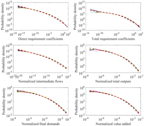
Fig. 3. Probability density distribution fits of pooled global economic data from WIOD during 1995–2009. The black dashed line represents the pooled data, and the red dashed line represents the best-fit distribution to the pooled data. Each solid line represents a country. Intermediate flows and industrial total outputs are normalized by total through-flow of the economy which is the sum of all industrial total outputs. Industrial final demands are normalized by the sum of all industrial final demands representing total final demand of the economy. Industrial value added is normalized by the sum of all industrial value added representing gross domestic products (GDP) of the economy. (For interpretation of the references to color in this figure legend, the reader is referred to the web version of this article.)
distribution for pooled data [7]. Our results agree with their findings, as Weibull distribution has larger log-likelihood value (1,087,370) than Log-normal distribution (1,085,760).
Fig. 3shows probability density distribution fits of pooled IO data from WIOD during 1995–2009. Unlike the OECD data, WIOD considers international trade flows among countries and treats countries as parts of an integrated global economic system. Similarly, probability density distributions of node strengths and link weights are heavy-tailed and have significant curvature on the log–log axes. Distributions of different datasets are similar to one another. The best fit for probability density distributions of node strengths and link weights is Burr distribution (Table S5). Again, we find that four types of distributions are similar to one another and can be used to model probability densities of node strengths and link weights, including Burr, Log-Logistic, Log-normal, and Weibull distributions.
Figs. 2and3show that nodes and links are highly heterogeneous in global economy. This calls for further investigation on different roles that nodes and links play in the global economy, which represents a useful future research avenue.
Power law distributions have been found in many real-world networks [16]. Figure S1 shows power law distribution fits of pooled IO data for 29 individual countries from the OECD database. Industrial total outputs measuring node strengths follow a power law distribution, while the other five indicators do not. Figure S2 shows power law distribution fits of pooled IO data from WIOD during 1995–2009. Direct requirement coefficients measuring link weights follow a power law distribution, while the other five indicators do not. There is no indicator following power law distributions based on both the OECD and WIOD databases. However, the observed power-law distributions for specific indicators seem to describe only
∼
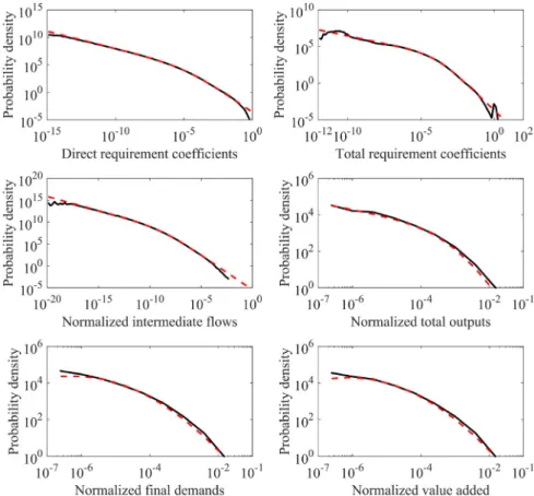
1% of the data. Thus, six indicators generally do not follow power law distributions. Details about the power law fitting are shown in the SI.Fig. 4. Probability density distribution fits of global economic data from WIOD in 2011. The black dashed line represents the global economic data, and the red dashed line represents the best-fit distribution to the data. Intermediate flows and industrial total outputs are normalized by total through-flow of the economy which is the sum of all industrial total outputs. Industrial final demands are normalized by the sum of all industrial final demands representing total final demand of the global economy. Industrial value added is normalized by the sum of all industrial value added representing gross domestic products (GDP) of the global economy. (For interpretation of the references to color in this figure legend, the reader is referred to the web version of this article.)
3.2. Impacts of dataset choice
We compare scaling patterns of the global economy derived from WIOD and Eora data in 2011 to examine how much impact dataset choice has on the results.Figs. 4,5, and6show probability density distribution fits of IO data from WIOD, Eora-original, and Eora-26, respectively, in 2011.
For WIOD data, the best fit for probability density distributions of link weights is Burr distribution (Table S6). For node strengths, the best fit for industrial total outputs is Burr distribution, while for industrial final demands and value added it is Log-normal distribution. This is generally consistent with results shown inFig. 3. In particular, we observe that fitted distributions for WIOD behave better for link weights than for node strengths (Fig. 4), as there are more data samples for the former.
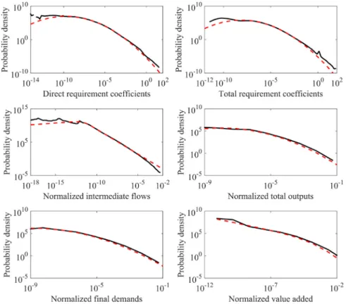
Best fits based on the Eora data (Tables S7 and S8) are different from those based on WIOD data. For Eora-original, the best fit for direct and total requirement coefficients is Log-normal distribution, while that for the other four indicators is Burr distribution. For Eora-26, the best fit for direct and total requirement coefficients, industrial total outputs, and industrial final demands is Log-normal distribution, and that for intermediate flows and industrial value added is Burr distribution.
We also find that, according to log-likelihood values in Tables S6, S7, and S8, whether based on WIOD or Eora data (including Eora-original and Eora-26), four types of distributions (i.e., Burr, Log-Logistic, Log-normal, and Weibull distributions) are similar to one another. This indicates that dataset choice has limited impacts on the scaling pattern of the global economy.
Fig. 5. Probability density distribution fits of global economic data from Eora-original in 2011. The black dashed line represents the global economic data, and the red dashed line represents the best-fit distribution to the data. Intermediate flows and industrial total outputs are normalized by total through-flow of the economy which is the sum of all industrial total outputs. Industrial final demands are normalized by the sum of all industrial final demands representing total final demand of the global economy. Industrial value added is normalized by the sum of all industrial value added representing gross domestic products (GDP) of the global economy. (For interpretation of the references to color in this figure legend, the reader is referred to the web version of this article.)
available directly from statistical agencies (e.g., National Statistical Institutes, OECD, and UN National Accounts statistics) [30,31]. Thus, it is generally expected that the quality of data for WIOD is better than that for Eora. This perhaps explains why WIOD performs better in distribution fits of link weights than Eora data.
In general, we find that dataset choice has limited impacts on the scaling pattern of the global economy, whether based on databases compiled by different organizations (i.e., WIOD versus Eora) or based on databases compiled by the same organization (i.e., Eora-original versus Eora-26). We also find that different compiling methods may result in different quality of IO data, but have limited impact on the scaling pattern of the global economy.
4. Discussion and conclusions
We examine scaling patterns of the global IO networks in this study. Probability density distributions of node strengths and link weights can be approximated by Burr, Log-Logistic, Log-normal, and Weibull distributions. We find that the best fits for probability densities of node strengths and link weights vary from different datasets. However, these four types of distributions generally perform well across all datasets. It is clear that global IO networks indeed have significant scaling patterns. Moreover, dataset choice has limited impacts on the observed scaling patterns. There are several real-world implications of this study.
Fig. 6. Probability density distribution fits of global economic data from Eora-26 in 2011. The black dashed line represents the global economic data, and the red dashed line represents the best-fit distribution to the data. Intermediate flows and industrial total outputs are normalized by total through-flow of the economy which is the sum of all industrial total outputs. Industrial final demands are normalized by the sum of all industrial final demands representing total final demand of the global economy. Industrial value added is normalized by the sum of all industrial value added representing gross domestic products (GDP) of the global economy. (For interpretation of the references to color in this figure legend, the reader is referred to the web version of this article.)
WIOD database can be used to assist data quality improvement of the Eora database in future. Specific data points in the Eora database that are outliers of the four types of distributions (i.e., Burr, Log-Logistic, Log-normal, and Weibull distributions) should be given special attention in future database improvements.
Second, scaling patterns of an economy are useful to predict missing data in economic statistics, using observed probability density distributions as the objective or a function of missing data prediction methods (e.g., linear optimization models [40]).
Third, scaling patterns of an economy show significant heterogeneity of nodes and links in an economy. This enables further investigation on identifying key nodes and links in IO networks and providing decision support for economic policies [2,3].
This study examines scaling patterns of global IO networks based on three widely used databases (i.e., OECD, WIOD, and Eora databases). Although these three databases are compiled by different organizations and have uncertainties to different extents, we found four common distribution functions to describe probability densities of their node strengths and link weights. This in turn proves that these common patterns are relatively robust. It is interesting to incorporate more global economic datasets in future studies.
Acknowledgment
Sai Liang and Shen Qu thank the support of the Dow Sustainability Fellows Program.
Appendix A. Supplementary data
Supplementary material related to this article can be found online athttp://dx.doi.org/10.1016/j.physa.2016.01.090.
References
[2] H.B. Chenery, T. Watanabe, International comparisons of the structure of production, Econometrica 26 (1958) 487–521. [3] E. Dietzenbacher, The measurement of interindustry linkages: Key sectors in the Netherlands, Ecol. Modell. 9 (1992) 419–437. [4] P.N. Rasmussen, Studies in Inter-Sectoral Relations, North-Holland Publishing Company, Amsterdam, Netherlands, 1956.
[5] F. Blöchl, F.J. Theis, F. Vega-Redondo, E.O.N. Fisher, Vertex centralities in input–output networks reveal the structure of modern economies, Phys. Rev. E 83 (2011) 046127.
[6] F. Cerina, Z. Zhu, A. Chessa, M. Riccaboni, World input–output network, 2014. arXiv PreprintarXiv:1407.0225. [7] J. McNerney, B.D. Fath, G. Silverberg, Network structure of inter-industry flows, Physica A 392 (2013) 6427–6441.
[8] M. Xu, B.R. Allenby, J.C. Crittenden, Interconnectedness and resilience of the US economy, Adv. Complex Syst. 14 (2011) 649–672.
[9] S. Liang, Y. Feng, M. Xu, Structure of the global virtual carbon network: Revealing important sectors and communities for emission reduction, J. Ind. Ecol. 19 (2015) 307–320.
[10]C.A. Hidalgo, B. Klinger, A.-L. Barabási, R. Hausmann, The product space conditions the development of nations, Science 317 (2007) 482–487. [11]M. Newman, The structure and function of complex networks, SIAM Rev. 45 (2003) 167–256.
[12]M. Newman, Networks: An Introduction, Oxford University Press, New York, 2010.
[13]R.E. Miller, P.D. Blair, Input-Output Analysis: Foundations and Extensions, Cambridge University Press, New York, 2009. [14]A.-L. Barabási, R. Albert, Emergence of scaling in random networks, Science 286 (1999) 509–512.
[15]L.A. Adamic, B.A. Huberman, A.L. Barabasi, R. Albert, H. Jeong, G. Bianconi, Power-law distribution of the world wide web, Science 287 (2000) 2115. [16]A. Clauset, C. Shalizi, M. Newman, Power-law distributions in empirical data, SIAM Rev. 51 (2009) 661–703.
[17]V.M. Eguíluz, D.R. Chialvo, G.A. Cecchi, M. Baliki, A.V. Apkarian, Scale-free brain functional networks, Phys. Rev. Lett. 94 (2005) 018102. [18]A. Klaus, S. Yu, D. Plenz, Statistical analyses support power law distributions found in neuronal avalanches, PLoS One 6 (2011) e19779. [19]G. Kossinets, D.J. Watts, Empirical analysis of an evolving social network, Science 311 (2006) 88–90.
[20]M. Lenzen, Aggregation versus disaggregation in input–output analysis of the environment, Econ. Syst. Res. 23 (2011) 73–89.
[21]A. Owen, K. Steen-Olsen, J. Barrett, T. Wiedmann, M. Lenzen, A structural decomposition approach to comparing MRIO databases, Econ. Syst. Res. 26 (2014) 262–283.
[22]W. Leontief, Recent developments in the study of interindustrial relationships, Amer. Econ. Rev. 39 (1949) 211–225. [23]W. Leontief, Input–output analysis as an alternative to conventional econometric models, Math. Social Sci. 25 (1993) 306–307. [24]W.W. Leontief, Quantitative input and output relations in the economic systems of the United States, Rev. Econ. Stat. 18 (1936) 105–125. [25]H.E. Stanley, Power laws and universality, Nature 378 (1995) 554.
[26]X. Gabaix, P. Gopikrishnan, V. Plerou, H.E. Stanley, Institutional investors and stock market volatility, Quart. J. Econ. 121 (2006) 461–504.
[27]D. Spasojević, S. Bukvić, S. Milošević, H.E. Stanley, Barkhausen noise: elementary signals, power laws, and scaling relations, Phys. Rev. E 54 (1996) 2531–2546.
[28]P.C. Ivanov, A. Yuen, B. Podobnik, Y. Lee, Common scaling patterns in intertrade times of US Stocks, Phys. Rev. E 69 (2004) 056107.
[29] OECD, STAN: OECD Structural Analysis Statistics (http://www.oecd-ilibrary.org/industry-and-services/data/stan-input–output_stan-in-out-data-en) in, Organisation for Economic Co-operation and Development, 2012.
[30]E. Dietzenbacher, B. Los, R. Stehrer, M. Timmer, G. de Vries, The construction of world input–output tables in the WIOD project, Econ. Syst. Res. 25 (2013) 71–98.
[31]M.P. Timmer, E. Dietzenbacher, B. Los, R. Stehrer, G.J. de Vries, An illustrated user guide to the world input–output database: the case of global automotive production, Rev. Int. Econ. 23 (2015) 575–605.
[32]M. Lenzen, D. Moran, K. Kanemoto, A. Geschke, Building Eora: a global multi-region input–output database at high country and sector resolution, Econ. Syst. Res. 25 (2013) 20–49.
[33] OECD, Producer Prices (MEI) (http://stats.oecd.org/Index.aspx?DataSetCode=MEI_PRICES_PPI) in, Organisation for Economic Co-operation and Development, 2014.
[34] WorldBank, Wholesale price index (http://data.worldbank.org/indicator/FP.WPI.TOTL), in, The World Bank, Washington, DC, USA, 2014.
[35] OECD, Monthly Monetary and Financial Statistics (MEI) (http://stats.oecd.org/index.aspx?queryid=6779), in, Organisation for Economic Co-operation and Development, 2014.
[36] R. Gibrat, Les Inégalités économiques. Paris, France, Paris, France, 1931.
[37]W. Leontief, A. Strout, Multi-regional Input-Output Analysis, in: T. Barna (Ed.), Structural Interdependence and Economic Development, St. Martin’s Press, New York, 1963.
[38]W. Liu, J. Chen, Z. Tang, H. Liu, D. Han, F. Li, Multi-Regional Input–Output Table Establishment Theory and Application of China’s 30 Provinces in 2007, China Statistics Press, Beijing, 2012.
[39]A. Parikh, Forecasts of input–output matrices using the RAS method, Rev. Econ. Stat. 61 (1979) 477–481.