Sharp global nonlinear stability for a fluid overlying a highly porous material

overlying a highly porous material

B y ANTONY A. HILL1 AND MAGDA CARR2

1_{School of Mathematical Sciences, University of Nottingham, Nottingham,}

NG7 2RD, UK

2_{School of Mathematics and Statistics, University of St Andrews, St Andrews,}

KY16 9SS, UK

The stability of convection in a two-layer system in which a layer of fluid with a temperature dependent viscosity overlies and saturates a highly porous material is studied. Due to the difficulties associated with incorporating the nonlinear advec-tion term in the Navier Stokes equaadvec-tions into a stability analysis, previous literature on fluid/porous thermal convection has modelled the fluid using the linear Stokes equations. This paper derives global stability for the full nonlinear system, by util-ising a model proposed by Ladyzhenskaya. The nonlinear stability boundaries are shown to be sharp when compared with the linear instability thresholds.

Keywords: superposed porous-fluid convection; temperature dependent viscosity; energy method

1. Introduction

Thermal convection within a two-layer system constructed by a layer of fluid over-lying a porous material saturated with the same fluid has numerous geophysical and industrial applications, such as the manufacturing of composite materials used in the aircraft and automobile industries, flow of water under the Earth’s surface, flow of oil in underground reservoirs and growing of compound films in thermal chemical vapor deposition reactors. A detailed review is given by Nield & Bejan (2006), with current highly relevant literature including Chen & Chen (1988), Ew-ing (1998), Blestet al. (1999), Straughan (2002, 2008), Carr (2004), Chang (2004, 2005, 2006), Hirataet al.(2007), Hoppeet al.(2007), Mu & Xu (2007) and Hill & Straughan (2009).

Assessing the onset and type of convection is crucial in understanding and con-trolling these geophysical and industrial processes. This is achieved by analyzing both the linear instability and nonlinear stability thresholds of the governing model. Comparing these thresholds allows the assessment of the suitability of linear the-ory to predict the physics of the onset of convection. The derivation of sharp un-conditional stability thresholds is particularly physically useful due to the lack of restrictions on the initial data (Straughan 2004).

in the Navier-Stokes equations into a stability analysis, the fluid is modelled using the linear Stokes equations.

This paper utilitses a model proposed by Ladyzhenskaya (Ladyzhenskaya 1967, 1968, 1969; Straughan 2002, 2004, 2008), which is used as an alternative to Navier-Stokes. This allows for the development of an unconditional nonlinear energy sta-bility analysis for thermal convection with temperature dependent viscosity in a fluid/porous system, without the need to remove the nonlinear advection term v_{· ∇}v_{. It is important to note that the viscosity of a liquid is usually strongly} dependent on temperature (cf. Capone & Gentile 1994, 1995; Galiano 2000). Con-vection problems for which the viscosity or conductivity is a function of temperature has received much recent attention in the literature (see e.g. Payne & Straughan 2000; Shevtsova et al. 2001; Manga et al. 2001), making this work particularly timely.

The stability calculations required to construct the neutral curves involve deter-mining eigenvalues and eigenfunctions, where the associated eigenvalue problems are not solvable analytically. The results are derived numerically using the Cheby-shev tau - QZ method (Dongarraet al. 1996), which is a spectral method coupled with the QZ algorithm. All numerical results were checked by varying the num-ber of polynomials to verify convergence. Standard indicial notation is employed throughout andk_{= (0, 0, 1).}

2. Formation of the problem

Consider a fluid occupying the three-dimensional layer{(x, y)∈R2} × {z∈(0, d)}

and saturating an underlying homogeneous porous medium{(x, y)∈R2} × {z ∈

(−dm,0)}.The interface between the saturated porous medium and the fluid is at

z= 0.

We assume that the dynamic viscosity µhas a linear temperature dependence of the form

µ(T) =µ0(1−γ(T−TL)),

for a constantγ >0, whereT, µ0 andTL are temperature and reference viscosity and temperature values, respectively. Although we only consider liquids which have a viscosity which decreases with increasing temperature, the analysis can be easily generalized to a more general viscosity-temperature relationship. The governing model for the fluid layer we select is

ρ0

µ

∂vi

∂t +vj ∂vi

∂xj

¶

= −∂p ∂xi

+ 2 ∂

∂xj

[(µ(T) +µ1|D_|)Dij]

−gρ0ki(1−α(T−TL)),

∂vi

∂xi

= 0, (2.1)

∂T ∂t +vj

∂T ∂xj

= κf

(ρ0cp)f

∇2_T,

of thermal expansion. A variation of this model was suggested by Ladyzhensakaya (1967, 1968, 1969) as an alternative to the Navier-Stokes equations, and is a gen-eralisation of a well known model in viscoelasticity (Antontsev et al. 2001). The parameter µ1 > 0 is a constant, Dij = (vi, j+vj, i)/2 and |D| =

p

DijDij. The subscripts (or superscripts)f andmdenote the fluid and porous layers respectively. In the porous medium we assume a high porosity φ > 0.75, such that the governing equations are given by

ρ0 φ

µ_∂vm i

∂t +

1

φv

m j

∂vm i

∂xj

¶

= −∂p

m

∂xi + 2

φ ∂ ∂xj

£

(µ(Tm_{) +µ1|D}m_|)Dm ij

¤

−µ(T

m₎

K v

m

i −gρ0ki(1−α(Tm−TL)),

∂vm i

∂xi

= 0, (2.2)

(ρ0cp)∗ (ρ0cp)f

∂Tm

∂t +v

m j

∂Tm

∂xj

= κ

∗

(ρ0cp)f

∇2Tm,

where the variables vm

i , pm, Tm and K are the velocity, pressure, temperature and permeability, respectively. The starred quantities are defined in terms of the fluid and porous variables such that S∗ _{= φS}

f + (1−φ)Sm, where S∗ = κ∗ or (ρ0cp)∗.A comprehensive discussion of the variances and various physical attributes of modelling transport through porous media is given in Alazmi & Vafai (2000).

The temperatures at the upper and lower boundaries are held fixed at TU and

TL, respectively, with continuity of temperature, velocity and heat flux at the in-terfacez = 0. The remaining boundary conditions atz = 0 are the continuity of normal stresses

−p+ 2(µ(T) +µ1|D_|)D33=−pm₊2

φ(µ(T

m_{) +µ1|D}m_|)Dm

33, (2.3)

and tangential stresses

(µ(T) +µ1|D_|)Dβ3= 1

φ(µ(T

m_{) +µ1|D}m_|)Dm

β3, (2.4)

forβ= 1, 2. The derivation of appropriate boundary conditions at the fluid/porous interface is non-trivial, cf. Vafai & Thiyagaraja (1987), Alazmi & Vafai (2001), Vafai (2005).

Under these boundary conditions, the governing equations (2.1) −(2.2) admit a steady state solution in which the velocity field is zero and

T = TL−

ǫT(TL−TU) ˆ

d+ǫT

− (TL−TU) dm( ˆd+ǫT)

z, z∈(0, d),

Tm = TL−

ǫT(TL−TU) ˆ

d+ǫT

−ǫT(TL−TU) dm( ˆd+ǫT)

z, z∈(−dm,0),

introduce the perturbations (ui, θ, π, umi , θm, πm),wheredij = (ui, j+uj, i)/2, and non-dimensionalisize with the scalings

ui=

µ0 ρ0du

∗

i, π=

µ2 0 ρ0d2π

∗

, θ=θ∗

s

µ3

0(TL−TU)

ρ3 0gαd3τf

, xi=dx∗i,

t= ρ0d

2 µ0 t

∗

, R=

s

gαρ0d3_(T

L−TU)

µ0τf

,

whereRa=R2 is the fluid Rayleigh number. By replacingdandτf bydmandτm, respectively, the porous layer scalings follow analogously, whereRm

a = (Rm)2is the porous Rayleigh number. This yields the non-dimensional perturbation equations

∂ui

∂t +uj ∂ui

∂xj

= −∂π ∂xi

+kiRθ− 2ΓP r

R ∂ ∂xj

(θdij) + 2ω

∂ ∂xj

(|d_|dij)

+2 ∂

∂xj

(f1dij),

∂ui

∂xi

= 0, (2.5)

P r

µ

∂θ ∂t +uj

∂θ ∂xj

¶

= RM1u3+∇2θ,

inR2×(0,1)×(0,∞) withf1= 1 + Γ(M2+M1z), dij = (ui, j+uj, i)/2 and

1

φ ∂um

i

∂t +

1

φ2u

m j

∂um i

∂xj

= −∂π

m

∂xi

+kiRmθm−

f2 δu

m i +

2 ˆd2_ω φ

∂ ∂xj

(|dm_|dm_ij)

+2

φ ∂ ∂xj

(f2dm ij) +

ΓP rǫT

Rm

µ₁

δu

m i θ

m₋2

φ ∂ ∂xj

(θm_dm ij)

¶

,

∂um i

∂xi

= 0, (2.6)

P rǫT

µ

Gm

∂θm

∂t +u

m j

∂θm

∂xj

¶

= Rm_M2um

3 +∇2θm,

in R2×(−1, 0)×(0,∞), with f2 = 1 + ΓM2(1 +z), dm

ij = (umi, j+umj, i)/2. The remaning parameters are the Prandtl numberP r =µ0/(κfρ0),Darcy numberδ=

K/d2

m, ω=µ1/(ρ0d2),Γ =γ(TL−TU), Gm= (ρ0cp)∗/(ρ0cp)f, M1 = ˆd/( ˆd+ǫT) andM2 =ǫT/( ˆd+ǫT).

3. Linear Instability Analysis

To proceed with a linear analysis, the nonlinear terms from (2.5) and (2.6) are discarded. We assume normal modes of the form

ui=ui(z)eσt+i(a1x+a2y), π=π(z)eσt+i(a1x+a2y), θ=θ(z)eσt+i(a1x+a2y),

with analogous definitions in the porous medium. Taking the double curls of (2.5)1

to the linearised equations

f1(D2−a2)2w+ 2ΓM1(D2−a2)Dw−a2Rθ = σ(D2−a2)w

(D2_−a2_{)θ+RM1w = P rσθ} f2

φ(D 2_−a2

m−

φ δ)(D

2_−a2

m)w m

+ 2ΓM2

φ (D 2_−a2

m−

φ

2δ)Dw

m

−a2mR m

θm = σ m

φ (D 2_−a2

m)w m

(D2−a2m)θm+RmM2wm = P rσmǫTGmθm

whereD= d/dz, a2_=a2

1+a22anda2m= (am1)2+ (am2)2.The boundary conditions

for the twelfth order system atz = 1 are

w=Dw=θ= 0,

and

wm_=Dwm_=θm_{= 0}

atz =−1.On the interface z= 0, we have

w= ˆdw, Dw= ˆd2Dwm_,

φ(D2_+a2_{)w= ˆd}3_(D2_+a2

m)w

m_{, θ=}q_ǫ Tdˆ3θm,

Dθ=

s

ˆ

d5 ǫT

Dθm,

and

f1(D2_−3a2_{)Dw+ ΓM1(D}2_+a2_)w−σDw=dˆ4f2 φ (D

2_−3a2

m)w m₊

ˆ

d4ΓM2 φ (D

2_+a2

m)w

m₋f2dˆ4

δ Dw

m₋dˆ4σm

φ Dw

m_.

The numerical results are presented in§5.

4. Nonlinear Stability Analysis

Let us define Ωf and Ωmto represent the period cells in the fluid and porous layers respectively, and introduce the notation of norm and inner product on the spaces

L2_(Ω

f) andL2(Ωm), where

kf||2

α=

Z

Ωα

fifidΩα, (f, g)α=

Z

Ωα

figidΩα, α=f, m.

the period cell. An analogous process is applied to (2.6)1and (2.6)3.We may now

define the functionalE(t) by

2E(t) =ku_k2_{f +λ1P rkθk}2_f+λ2

φku

m_k2

m+λ3ǫTGmP rkθmk2m,

for coupling parametersλ1, λ2, λ3>0,such that

dE

dt = (ui, [−ujui, j−π, i+kiRθ−

2ΓP r

R (θdij), j+ 2ω(|d|dij), j+ 2(f1dij), j])f

+λ1(θ, [−P ruiθ, i+RM1w+∇2θ])f+λ2(umi , [− 1

φ2u

m j u

m i, j−π

m

, i (4.1)

+kiRmθm−

f2 δ u

m i −

2ΓP rǫT

φRm (θ m_dm

ij), j+ ΓP rǫT

δRm θ m_um

i + 2 ˆd2_ω

φ (|d

m_|dm ij), j

+2

φ(f2d

m

ij), j])m+λ3(θm, [−ǫTP ruimθ, im+RmM2wm+∇2θm])m.

Utilising a similar approach to Hill & Straughan (2009), the first and third terms on the right hand side of (4.1) are integrated by parts, and the nondimensionalised versions of boundary condtions (2.3) and (2.4) are employed to yield

(ui, [−ujui, j−π, i− 2ΓP r

R (θdij), j+ 2ω(|d|dij), j+ 2(f1dij), j])f

+λ2(um i , [−

1

φ2u

m j u

m i, j−π

m , i −

2ΓP rǫT

φRm (θ m_dm

ij), j+ 2 ˆd2_ω

φ (|d

m_|dm ij), j+

2

φ(d

m ij), j])m

= 1 2

Z

Λ

Ã

|u_|2_w− dˆ

3 φ2|u

m_|2_wm

!

dS−2ω

Z

Ωf

|d_|3_dΩf−2

Z

Ωf

f1|d_|2_dΩf

+2ΓP r

R

Z

Ωf

θ|d_|2_dΩf−2 ˆd

5_ω φ

Z

Ωm

|dm_|3_dΩm−2 ˆd

3 φ

Z

Ωm

f2|d_|2_dΩm

+2ΓP rǫTdˆ

3 φRm

Z

Ωm

θm_|dm_|2_dΩ

m,

whereλ2= ˆd3_{,and Λ represents the fluid/porous interface atz = 0. Similarly, by}

integrating by parts and utilising the non-dimensionalised boundary conditions

λ1(θ, [−P ruiθ, i+∇2θ])f + λ3(θm, [−P rǫTumi θm, i+∇2θm])m = −λ(k∇θk2f+ ˆd4k∇θmk2m)

Combining these definitions it follows that

dE

dt =

1 2

Z

Λ

Ã

|u_|2_w−dˆ

3 φ2|u

m

|2wm

!

dS+R < θ, w >−2ω

Z

Ωf

|d_|3_dΩf

−2

Z

Ωf

f1|d_|2_dΩf+2ΓP r

R

Z

Ωf

θ|d_|2_{dΩf−λk∇θk}2_{+λRM1< w, θ >}

+ ˆd3Rm< θm, umi >− ˆ

d3 δ

Z

Ωm

f2|um_|2_dΩm+ΓP rǫTdˆ

3 δRm

Z

Ωm

θm|um_|2_dΩm

−2 ˆd 5_ω φ

Z

Ωm

|dm_|3_dΩm−2 ˆd

3 φ

Z

Ωm

f2|dm_|2_{dΩm (4.2)}

+2ΓP rǫTdˆ

3 φRm

Z

Ωm

θm|dm_|2_dΩm+Rm_dˆ4_{M2λ < w}m_{, θ}m_>−λdˆ4_k∇θm_k2_.

To address the cubic nonlinearities in (4.2) we introduce the L3 _{norm k · k3.}

Multiplying (2.5)₃ and (2.6)₃ by θ2 _{and (θ}m₎2_{, respectively, integrating over the}

period cell, and using Poincar´e’s inequality we find

λ4P r

3

d dtkθk

3 3 +

λ5P rǫTGm 3

d dtkθ

m_k3

3≤λ4RM1

Z

Ωf

wθ2(sgn θ)dΩf

+λ4ǫ 1 2 Tdˆ

11 2 RM2

Z

Ωm

wm_(θm₎2_{(sgn θ}m_)dΩ m

−8π 2_λ4

9

Z

Ωf

|θ3|dΩf−

8π2_λ4ǫ12 Tdˆ

11 2

9

Z

Ωm

|θm_|3_dΩ

m, (4.3)

where λ5 = λ4ǫ 1 2 Tdˆ

11

2 to ensure the removal of the boundary integrals (Hill &

Straughan 2009). We now use Young’s inequality on the cubic integral terms in both (4.2) and (4.3), such that

Z

Ω

Q1Q22dΩ≤ c2

3kQ1k

3 3+

1 3ckQ2k

3 3

forc >0, whereQ16=Q2.

Letting

E1= 1 2E+

λ4P r

3 kθk

3 3+

λ5P rǫTGm

3 kθ

m

and combining (4.2) and (4.3) we now have

dE1

dt ≤ R(1 +λM1)< θ, w >f −2

Z

Ωf

f1|d_|2_{dΩf −λk∇θk}2_f−dˆ

3 δ

Z

Ωm

f2|um_|2_dΩm

− 2 ˆd 3 φ

Z

Ωm

f2|dm_|2_dΩm−λdˆ4_k∇θm_km2 _+Rm_dˆ3_{(1 +λM2d}ˆ_{)< θ}m_{, w}m_>m

+ 1

2

Z

Λ

Ã

|u_|2_w−dˆ

3 φ2|u

m_|2_wm

!

dS+RM1β

2 1λ4

3

Z

Ωf

|u3_|dΩf

+

Ã

Rm_M2β2 2ǫ

1 2 Tdˆ

11 2λ4

3 +

2ΓP rǫTdˆ3 3δRm_α2

3

! Z

Ωm

|um_|3_{dΩm (4.4)}

−

µ_8π2_λ4

9 −

2RM1λ4

3β1 −

2ΓP rα1

3R

¶ Z

Ωf

|θ|3dΩf

−

µ

2ω−4ΓP r

3α2 1R

¶ Z

Ωf

|d_|3_dΩf−

Ã

2ωdˆ5 φ −

4ΓP rǫTdˆ3 3α2

2Rmφ

! Z

Ωm

|dm_|3_dΩm

−

Ã

8π2_λ4ǫ12 Tdˆ

11 2

9 −

2Rm_M2λ4ǫ12 Tdˆ

11 2

3β2 −

ΓP rǫTdˆ3 3Rm

µ

2α2 φ +

α3 δ

¶!Z

Ωm

|θm_|3_dΩ

m,

where αi, βj are positive constants for i = 1, 2, 3; j = 1, 2 introduced by using Young’s inequality on the cubic terms. Before we choose the coefficients to bind the cubicd_{, θ,}dm_andθm_{integrals, we must address the boundary integrals and cubic} u_andum_{terms in (4.4).}

To achieve this we utilise the following Poincar´e like inequalities:

Z

Ωf

|u_|3_{dΩf ≤c1}

Z

Ωf

|d_|3_{dΩf (4.5)}

and

Z

Λ

|u_|3_dS+c2

Z

Ωf

|u_|3_{dΩf ≤c3}

Z

Ωf

|d_|3_{dΩf, (4.6)}

where c1, c2, c3 >0. Similar inequalities follow in the porous case, for constants

cm

given in Appendix A. Applying (4.5) and (4.6) to (4.4) yields

dE1

dt ≤ R(1 +λM1)< θ, w >f −2

Z

Ωf

f1|d_|2_{dΩf−λk∇θk}2_f−dˆ

3 δ

Z

Ωm

f2|um_|2_dΩm

−2 ˆd 3 φ

Z

Ωm

f2|dm_|2_dΩm−λdˆ4_k∇θm_km2 _+Rm_dˆ3_{(1 +λM2d}ˆ_{)< θ}m_{, w}m_>m

−

µ_8π2_λ4

9 −

2RM1λ4

3β1 −

2ΓP rα1

3R

¶ Z

Ωf

|θ|3dΩf

−

µ

2ω−4ΓP r

3α2 1R

−RM1β 2 1λ4c1

3 −

c3−c1c2

2

¶ Z

Ωf

|d_|3_{dΩf (4.7)}

−

Ã

2ωdˆ5 φ −

2ΓP rǫTdˆ3 3Rm

µ ₂ φα2 2 + c m 1 δα2 3 ¶ −R

m_M2β2 2ǫ

1 2 Tdˆ

11 2λ4cm

1

3

−dˆ 3_(cm

3 −cm1cm2)

2φ2

! Z

Ωm

|dm_|3_dΩm

−

Ã

8π2_λ4ǫ12 Tdˆ

11 2

9 −

2Rm_M2λ4ǫ12 Tdˆ

11 2

3β2 −

ΓP rǫTdˆ3 3Rm

µ_2α2

φ + α3

δ

¶!Z

Ωm

|θm|3dΩm.

Now putλ4=λ′

4+kε, and let

8π2_λ′

4

9 −

2RM1λ′

4

3β1 −

2ΓP rα1

3R = 0,

8π2_λ′

4ǫ 1 2 Tdˆ

11 2

9 −

2Rm_M2λ′

4ǫ 1 2 Tdˆ

11 2

3β2 −

ΓP rǫTdˆ3 3Rm

µ 2α2 φ + α3 δ ¶

= 0,

which is satisfied for

β2=β1

µ_ǫ3

T ˆ d5 ¶ 1 2

, 2α2 φ +

α3

δ = 2α1d,ˆ λ

′

4=

3ΓP rα1β1

4π2_Rβ1−3R2_M1.

We now minimize

4ΓP r

3α2 1R

+ ΓP rα1M1β

2 1c1

4π2_β1−3RM1

with respect toα1andβ1 to yield

α1= 8π

2₄1 3

9RM1c 1 3 1

, β1= 9RM1 8π2 ,

and chooseα3to minimize

2ΓP rǫTdˆ3 3Rm

From (4.7), choosingk= 27/(8π2_{) we can now deduce}

dE1

dt ≤ R(1 +λM1)< θ, w >f −2

Z

Ωf

f1|d_|2_{dΩf −λk∇θk}2_f−dˆ

3 δ

Z

Ωm

f2|um_|2_dΩm

−2 ˆd 3 φ

Z

Ωm

f2|dm_|2_dΩm−λdˆ4_k∇θm_km2 _+Rm_dˆ3_{(1 +λM2d}ˆ_{)< θ}m_{, w}m_>m

−ε

Z

Ωf

|θ|3dΩf−ωˆ

Z

Ωf

|d_|3_dΩf−ωˆm

Z

Ωm

|dm_|3_dΩm−εǫ 1 2 Tdˆ

11 2

Z

Ωm

|θm|3dΩm,

where we require

ˆ

ω = 2ω−81ΓP r4 1 3RM2

1c 2 3 1

64π4 −

c3−c1c2

2 −ε

729R3_M3 1c1

512π6 >0

ˆ

ωm ₌ 2ωdˆ5

φ −

2ΓP rǫTdˆ3 3Rm

µ ₂ φα2 2 + c m 1 δα2 3 ¶

−27ΓP r4 1 3RmM2

2cm1ǫ 5 2 Tdˆ

3 2

32π4_c13 1

(4.8)

−dˆ 3_(cm

3 −cm1cm2 )

2φ2 −ε

729(Rm₎3_M3 2cm1 ǫ

1 2 Tdˆ

11 2

512π6 >0.

Defining

I = R(1 +λM1)< θ, w >f +Rmdˆ3(1 +λM2dˆ)< θm, wm>m,

D = 2

Z

Ωf

f1|d_|2_{dΩf +λk∇θk}2_f+dˆ

3 δ

Z

Ωm

f2|um_|2_dΩm

+2 ˆd

3 φ

Z

Ωm

f2|dm_|2_dΩm+λdˆ4_k∇θm_k2_m,

it follows that

dE1

dt ≤ −D

µ_R

E−1

RE

¶

−ε

Z

Ωf

|θ|3dΩf−εǫ 1 2 Tdˆ

11 2

Z

Ωm

|θm|3dΩm,

where 1 RE = max H µ_I D ¶

<1. (4.9)

Utilising Poincar´e like inequalities (cf. Payne & Straughan 1998) allows us to deduce that

dE1

dt ≤ −mE1

where m > 0. Integrating, we have E1(t) ≤ E1(0)e−mt _{→ 0 as t → ∞, where} convergence is at least exponential, so we have established unconditional nonlinear stability provided (4.8) and (4.9) hold.

The corresponding Euler Lagrange equations which arise at the sharpest thresh-oldRE = 1 are

2f1∇2_u

i+ 2f1′w, i+ 2f1′ui,3+kiR(M1λ+ 1)θ=L, i

in the fluid layer, and

2δdˆ3_(f2∇2_um i +f

′

2w, im+φf

′

2umi,3)−2φdˆ3f2umi +kiφδRmdˆ3(M2λdˆ+ 1)θm=φδLm, i 2λd∇ˆ 2θm_+Rm_{(M2λdˆ+ 1)w}m_{= 0}

(4.11) in the porous layer, whereLandLm _{are Lagrange multipliers.}

By taking the doublecurl of equations (4.10)1and (4.11)1and adopting normal

mode representations, the twelfth-order eigenvalue problem (4.10) – (4.11) can be utilised to locate the critical nonlinear Rayleigh numberRaE,which is given by

RaE= max λ mina2 R

2_(a2_{, λ).}

Numerical results for the nonlinear energy approach are presented in§5.

5. Results and conclusions

The first key result that can be derived is for the case Γ = 0, which corresponds to the viscosity of the fluid being constant with respect to temperature. Under this condition the equations for linear instability and nonlinear stability are identical to those of Hill & Straughan (2009), for which excellent agreement was shown between the two. It is important to note, though, that in this paper the nonlinear advection termv_{· ∇}v _{is included in the analysis, whereas the analysis of Hill & Straughan} (2009) is limited to the nonlinear Stokes problem.

For Γ 6= 0 we now solve the eigenvalue problem (4.10) − (4.11) by means of a D2 _{Chebyshev tau method. The details are similar to those given by Dongarra}

et al.(1996). The parameters, unless stated otherwise, are fixed at δ= 5×10−6_, Gm = 10, P r = 6 and ǫT = 0.7. The porous material is assumed to be that of a Foametal (which is used extensively in industrial applications such as heat exchangers, chemical reactors and fluid filters), with physical values of permeability and porosity of 8.19×10−8_m2 _{and 0.79, respectively (cf. Straughan 2002, Goyeau}

et al.2003).

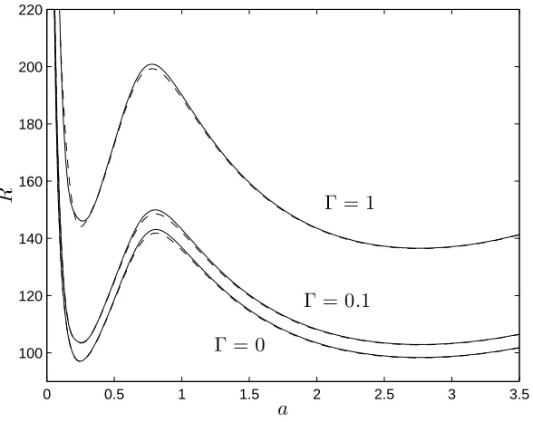
Figure 1 shows the neutral curves for a variation of Γ values, where the linear instability and nonlinear stability thresholds are represented by solid and dashed lines respectively.

It is clear that an increase in Γ causes the system to become more stable. Assuming that the temperature at the boundaries remains fixed, this corresponds to the strength of the linear dependence of viscosity on temperature increasing. As the viscosity decreases with an increase in temperature, this physcially makes sense. An interesting result is that the bimodal nature of the neutral curve is unaffected by the change in Γ.

Since the linear instability and nonlinear stability results clearly show excel-lent agreement, we can conclude that the linear theory accurately encapsulates the physics of the onset of convection.

Appendix A. A proof of inequalities

(4.5)

and

(4.6)

0 0.5 1 1.5 2 2.5 3 3.5 100

120 140 160 180 200 220

a

R

Γ = 0

Γ = 0

_.

1

Γ = 1

Figure 1. Visual representation of linear instability (solid lines) and nonlinear stabil-ity (dashed lines) thresholds, with critical thermal Rayleigh number R plotted against wavenumbera,for Γ = 0, 0.1 and 1. The remaining parameters are ˆd= 0.116,P r = 6, andφ= 0.79.

∂Ωf = Λ + Λ0.In the same vein as§4, Λ represents the fluid/porous interface atz = 0. For aC1 _functionf

i to be chosen at our discretion, we observe that

Z

Λ

fini|u|3dS=

Z

Ωf

fi, i|u|3dΩf+ 3

Z

Ωf

fi|u|ujuj, idΩf

and

3

Z

Λ

finj|u|ujuidS= 3

Z

Ωf

fi|u|, jujuidΩf

+3

Z

Ωf

fi|u|ujui, jdΩf+ 3

Z

Ωf

fi, j|u|ujuidΩf.

By letting

f _{= (−p1x,−p1y,−p1z−p2),}

wherep1 andp2are constants to be chosen at our discretion, it follows that

p2

Z

Λ

|u_|3_dS−3

Z

Λ

fiui|u|w dS+ 6p1

Z

Ωf

|u_|3_dΩf

= 3

Z

Ωf

fi|u|uj(ui, j+uj, i)dΩf+ 3

Z

Ωf

The arithmetic-geometric mean inequality leads us to

Z

Λ

xβuβw|u|dS≤

d1

2

µ

1

α

Z

Λ

w2|u_|dS+α

Z

Λ

u2β|u|dS

¶

where α >0 is a constant, andd1 = maxi=1,2(1,|xi|). Employing this inequality yields

µ

4p2−3p1d1

2α

¶ Z

Λ

w2_|u|dS+

µ

p2−3p1d1α

2

¶ Z

Λ u2

β|u|dS+ 6p1

Z

Ωf

|u_|3_dΩf

≤3

Z

Ωf

fi|u|uj(ui, j+uj, i)dΩf+ 3

Z

Ωf

fi|u|, jujuidΩf. (A 1)

Lettingα= 1/2 andp2= 3p1d1/4 to remove the boundary integrals, we now have

6p1

Z

Ωf

|u_|3_{dΩf ≤} 63p1d1 4

Z

Ωf

|u_|2_|d_|dΩf.

By using the Cauchy-Schwartz inequality on the right hand side, we find

Z

Ωf

|u_|3_{dΩf ≤}

µ_21d1

8

¶3Z

Ωf

|d_|3_dΩf,

which is inequality (4.5).

To derive inequality (4.6) we return to (A 1). By letting

p2=p1d1 2α (1−α

2_),

and using (4.5) it follows that

Z

Λ

|u_|3_{dΛ +} 12α

d1(1−4α2₎

Z

Ωf

|u_|3_{dΩf ≤} 9(21d1)

2_(2α−α2_{+ 1)}

64(1−4α2₎

Z

Ωf

|d_|3_dΩf

as required, whereαis a constant to be chosen at our discretion.

References

Alazmi, B. & Vafai, K. 2000 Analysis of variants within the porous media transport models.

ASME J. Heat Transfer 122_{, 303–326.}

Alazmi, B. & Vafai, K. 2001 Analysis of fluid flow and heat transfer interfacial conditions between a porous medium and a fluid layer.Int. J. Heat Mass transfer44_{, 1735–1749.}

Antontsev, S., Diaz, J. & Shmarev, S. 2001Energy methods for free boundary problems.

Boston: Birkhauser.

Blest, C., Duffy, B. R., Mckee, S. & Zulkfle, A. K. 1999 Curing simulation of thermoset composites.Composites, Part A30_{, 1289–1309.}

Capone, F. & Gentile, M. 1994 Nonlinear stability analysis of convection for fluids with exponentially temperature-dependent viscosity.Acta Mech.107_{, 53-64.}

Carr, M. 2004 Penetrative convection in a superposed porous-medium-fluid layer via in-ternal heating.J. Fluid Mech.509_{, 305–329.}

Chang, M. H. 2004 Stability of convection induced by selective absorption of radiation in a fluid overlying a porous layer.Phys. Fluids16_{, 3690–3698.}

Chang, M. H. 2005 Thermal convection in superposed fluid and porous layers subjected to a horizontal plane Couette flow.Phys. Fluids17_{, 064106-1–064106-7.}

Chang, M. H. 2006 Thermal convection in superposed fluid and porous layers subjected to a plane Poiseuille flow.Phys. Fluids18_{, 035104-1–035104-10.}

Chen, F. & Chen, C. F. 1988 Onset of finger convection in a horizontal porous layer underlying a fluid layer.J. Heat Transfer110_{, 403–409.}

Dongarra, J. J., Straughan, B. & Walker, D.W. 1996 Chebyshev tau-QZ algorithm meth-ods for calculating spectra of hydrodynamic stability problems.App. Num. Math.22_,

399–434.

Ewing, E. & Weekes, S. 1998 Numerical methods for contaminant transport in porous media.Comput. Math.202_{, 75–95.}

Galiano, G. 2000 Spatial and time localization of solutions of the Boussinesq system with nonlinear thermal diffusion.Nonlin. Analysis 42_{, 423-438.}

Goyeau, B., Lhuillier, D., Gobin, D. & Velarde M. G. 2003 Momentum transport at a fluid-porous interface.Int. J. Heat Mass Trans.46_{, 4071–4081.}

Hill, A. A. & Straughan, B. 2009 Global stability for thermal convection in a fluid overlying a highly porous material.Proc Roy Soc A465_{, 207–217.}

Hirata, S. C., Goyeau, B., Gobin, D., Carr, M. & Cotta, R. M. 2007 Linear stability of natural convection in superposed fluid and porous layers: influence of the interfacial modelling.Int. J. Heat Mass Transfer 50_{, 1356–1367.}

Hoppe, R. H. W., Porta, P. & Vassilevski, Y. 2007 Computational issues related to iterative coupling of subsurface and channel flows.Calcolo 44_{, 1–20.}

Ladyzhenskaya, O. A. 1967 New equations for the description of motions of viscous in-compressible fluids and global solvability of their boundary value problems.Tr. Mat. Inst. Steklova102_{, 85-104.}

Ladyzhenskaya, O. A. 1968 On some nonlinear problems in the theory of continuous media.

Am. Math. Soc. Transl. 2 70_{, 73-89.}

Ladyzhenskaya, O. A. 1969The mathematical theory of viscous incompressible flow, 2nd edn. New York: Gordon and Breach.

Manga, M., Weeraratne, D. & Morris, S. J. S. 2001 Boundary-layer thickness and insta-bilities in B´enard convection of a liquid with a temperature-dependent viscosity.Phys. Fluids13_{, 802–805.}

Mu, M. & Xu, J.C. 2007 A two-grid method of a mixed Stokes – Darcy model for coupling fluid flow with porous medium flow.SIAM J. Numer. Anal.45_{, 1801–1813.}

Nield, D. A. & Bejan, A. 2006Convection in porous media, 3rd edn. New York: Springer-Verlag.

Payne, L. E. & Straughan, B. 1998 Analysis of the boundary condition at the interface between a viscous fluid and a porous medium and related modelling questions.J. Math. Pures Appl.77_{, 317–354.}

Payne, L. E. & Straughan, B. 2000 Unconditional nonlinear stability in temperature-dependent viscosity flow in a porous medium.Stud. Appl. Math.105_{, 59–81.}

Payne, L. E., Song, J. C. & Straughan, B. 1999 Continuous dependence and convergence results for Brinkman and Forchheimer models with variable viscosity.Proc. Roy. Soc. London A455_{, 2173–2190.}

Straughan, B. 2002 Sharp global nonlinear stability for temperature-dependent viscosity convection.Proc Roy Soc A458_{, 1773–1782.}

Straughan, B. 2004 The energy method, stability and nonlinear convection. New York: Springer.

Straughan, B. 2008Stability and wave motion in porous media.Appl. Math. Sci. Ser. vol.

165_{. New York: Springer.}

Vafai, K. 2005Handbook of Porous Media.2nd edition, New York: Taylor & Francis. Vafai, K. & Thiyagaraja, R. 1987 Analysis of flow and heat transfer at the interface region