Submitted3 January 2017
Accepted 10 April 2017
Published17 May 2017
Corresponding author
Matthew Spencer, [email protected]
Academic editor
Mark Hay
Additional Information and Declarations can be found on page 19
DOI10.7717/peerj.3290 Copyright
2017 Allen et al.
Distributed under
Creative Commons CC-BY 4.0 OPEN ACCESS
Among-site variability in the stochastic
dynamics of East African coral reefs
Katherine A. Allen1,2, John F. Bruno3
, Fiona Chong1
, Damian Clancy4
, Tim R. McClanahan5
, Matthew Spencer1
and Kamila Żychaluk6
1School of Environmental Sciences, University of Liverpool, Liverpool, United Kingdom 2Institute of Integrative Biology, University of Liverpool, Liverpool, United Kingdom 3Department of Biology, University of North Carolina at Chapel Hill, Chapel Hill, NC,
United States of America
4School of Mathematical and Computer Sciences, Actuarial Mathematics and Statistics, Heriot-Watt
University, Edinburgh, United Kingdom
5Wildlife Conservation Society, NY, United States of America
6Department of Mathematical Sciences, University of Liverpool, Liverpool, United Kingdom
ABSTRACT
Coral reefs are dynamic systems whose composition is highly influenced by unpre-dictable biotic and abiotic factors. Understanding the spatial scale at which long-term predictions of reef composition can be made will be crucial for guiding conservation efforts. Using a 22-year time series of benthic composition data from 20 reefs on the Kenyan and Tanzanian coast, we developed Bayesian vector autoregressive state-space models for reef dynamics, incorporating among-site variability, and quantified their long-term behaviour. We estimated that if there were no among-site variability, the total long-term variability would be approximately one-third of its current value. Thus, our results showed that among-site variability contributes more to long-term variability in reef composition than does temporal variability. Individual sites were more predictable than previously thought, and predictions based on current snapshots are informative about long-term properties. Our approach allowed us to identify a subset of possible climate refugia sites with high conservation value, where the long-term probability of coral cover ≤0.1 (as a proportion of benthic cover of hard substrate) was very low. Analytical results show that this probability is most strongly influenced by among-site variability and by interactions among benthic components within sites. These findings suggest that conservation initiatives might be successful at the site scale as well as the regional scale.
SubjectsEcology, Marine Biology, Mathematical Biology
Keywords Vector autoregressive model, State-space model, Stochastic dynamics, Community composition, Spatial variability, Temporal variability, Coral reef, Bayesian statistics
INTRODUCTION
‘‘Probabilistic language based on stochastic models of population growth’’ has been proposed as a standard way to evaluate conservation and management strategies (Ginzburg
et al., 1982). For example, a stochastic population model can be used to estimate the
probability of abundance falling below some critical level. Such population viability analyses are widely used, and may be reasonably accurate if sufficient data are available
(Brook et al., 2000). In principle, the same approach could be used for communities,
A good candidate for such a model is the vector autoregressive model of order 1 or VAR(1) (Lütkepohl, 1993;Ives et al., 2003). This is a discrete-time model for the vector of log abundances of a set of species or groups, which includes environmental stochasticity and may include environmental explanatory variables. It makes the simplifying assumptions that inter- and intraspecific interactions can be represented by a linear approximation on the log scale, and that future abundances are conditionally independent of past abundances, given current abundances. Where possible, it is desirable to use a state-space form of the VAR(1) model, which also includes measurement error (Lindegren et al., 2009;Mutshinda, O’Hara & Woiwod, 2009).
Hampton et al. (2013) review applications of VAR(1) models in community ecology,
which include studying the stability of freshwater plankton systems (Ives et al., 2003), designing adaptive management strategies for the Baltic Sea cod fishery (Lindegren et
al., 2009), and estimating the contributions of environmental stochasticity and species
interactions to temporal fluctuations in abundance of moths, fish, crustaceans, birds and rodents (Mutshinda, O’Hara & Woiwod, 2009). Recently, VAR(1) models have been applied to the dynamics of the benthic composition of coral reefs (Cooper, Spencer & Bruno, 2015;Gross & Edmunds, 2015), using a log-ratio transformation (Egozcue et al., 2003) rather than a log transformation, to deal with the constraint that proportional cover of space-filling benthic groups sums to 1.
Coral reefs are dynamic systems influenced by both deterministic factors such as interactions between macroalgae and hard corals (Mumby, Hastings & Edwards, 2007), and stochastic factors such as temperature fluctuations (Baker, Glynn & Riegl, 2008) and storms (Connell, Hughes & Wallace, 1997), and are classic examples of non-equilibrium systems whose diversity is determined by both interspecific interactions and disturbance (Huston, 1985). In general, high coral cover is considered a desirable state for a coral reef, and there is some evidence that coral cover of at least 0.1 (as a proportion of substrate, equivalent to 10%) is important for long-term maintenance of reef function (Kennedy et al., 2013;Perry et al., 2013;Perry et al., 2015;Roff, Zhao &
Mumby, 2015). A positive net carbonate budget is necessary to maintain reef functions
such as provision of habitat (Kennedy et al., 2013). Simulation models of Caribbean reefs suggested that coral cover of 0.1 was just sufficient to maintain a zero net carbonate budget under a scenario with low greenhouse gas emissions and protection of herbivorous fish (Kennedy et al., 2013). Statistical analysis of field data from Caribbean reefs (Perry et
al., 2013) supported the idea that coral cover greater than 0.1 is required for a positive
There is evidence for systematic differences in reef dynamics among locations. For example, on the Great Barrier Reef up to 2012, coral cover had declined more strongly at southern and central than at northern sites (De’ath et al., 2012), and in the US. Virgin Islands, VAR(1) models showed that sites differed in their sensitivity to disturbance and speed of recovery (Gross & Edmunds, 2015). Some sites in a region may therefore represent coral refugia, where reefs are either protected from or able to adapt to changes in environmental conditions (McClanahan et al., 2007b). Alternatively, apparent differences among sites may simply be due to differences in recent acute disturbance history, and may not persist in the long term (e.g.,Connell, 1997). Although it may be possible to associate differences in dynamics among sites with differences in environmental variables, it is also possible to treat among-site differences as another random component of a VAR(1) model. This will allow estimation of the relative importance of among-site variability and within-site temporal variability, which is important for the design of conservation strategies. If within-site temporal variability dominates, it will not be possible to identify good sites to conserve based on current status, while if among-site variability dominates, even a ‘‘snapshot’’ sample at one time point may be enough to identify good sites. Thus, for example, the reliability of among-site patterns from surveys at one time point, such as the relationship between benthic composition and human impacts on remote Pacific atolls (Sandin et al., 2008), depends on among-site variability dominating within-site temporal variability. Thus, even though a simple strategy based on a snapshot may turn out to be effective, it is not possible to know this in advance of carrying out a more sophisticated analysis that treats the system as dynamic. As far as we know, the use of VAR(1) models to estimate spatiotemporal heterogeneity and identify refugia is novel, although other applications of VAR(1) models with random subject effects exist (e.g. Gorrostieta et al., 2012;Driver, Oud & Voelkle, 2016). Our approach differs from existing methods for identifying refugia (Keppel et al., 2012) in that it explicitly focuses on spatial variability in dynamics over ecological timescales, rather than on patterns that are static or vary only over much longer timescales. Furthermore, rather than differences in physical factors (West
& Salm, 2003), we focus on differences in community dynamics.
Here, we develop a state-space VAR(1) model for regional dynamics of East African coral reefs, including random site effects and measurement error, and use it to answer four key questions about spatial and temporal variability. How important is among-site variability in the dynamics of benthic composition, relative to within-site temporal variability? How much variability is there among sites in the probability of low (≤0.1) coral cover? Which model parameters have the largest effects on the probability of low coral cover in the region? How informative is a single snapshot in time about the long-term properties of a site?
METHODS
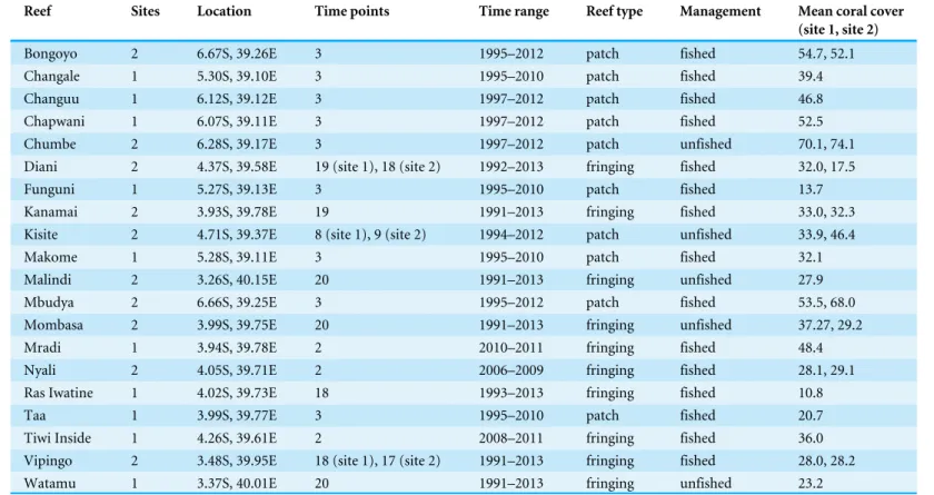
Data collectionTable 1 Sampling information and reef features.For each named reef, surveys were done at either one site, or at two sites 20 m–100 m apart. Fished reefs include community management areas with reduced harvesting intensity, and unfished reefs include those recently designated as re-serves. Mean coral cover is the arithmetic mean of observed coral cover over all transects and time points.
Reef Sites Location Time points Time range Reef type Management Mean coral cover
(site 1, site 2)
Bongoyo 2 6.67S, 39.26E 3 1995–2012 patch fished 54.7, 52.1
Changale 1 5.30S, 39.10E 3 1995–2010 patch fished 39.4
Changuu 1 6.12S, 39.12E 3 1997–2012 patch fished 46.8
Chapwani 1 6.07S, 39.11E 3 1997–2012 patch fished 52.5
Chumbe 2 6.28S, 39.17E 3 1997–2012 patch unfished 70.1, 74.1
Diani 2 4.37S, 39.58E 19 (site 1), 18 (site 2) 1992–2013 fringing fished 32.0, 17.5
Funguni 1 5.27S, 39.13E 3 1995–2010 patch fished 13.7
Kanamai 2 3.93S, 39.78E 19 1991–2013 fringing fished 33.0, 32.3
Kisite 2 4.71S, 39.37E 8 (site 1), 9 (site 2) 1994–2012 patch unfished 33.9, 46.4
Makome 1 5.28S, 39.11E 3 1995–2010 patch fished 32.1
Malindi 2 3.26S, 40.15E 20 1991–2013 fringing unfished 27.9
Mbudya 2 6.66S, 39.25E 3 1995–2012 patch fished 53.5, 68.0
Mombasa 2 3.99S, 39.75E 20 1991–2013 fringing unfished 37.27, 29.2
Mradi 1 3.94S, 39.78E 2 2010–2011 fringing fished 48.4
Nyali 2 4.05S, 39.71E 2 2006–2009 fringing fished 28.1, 29.1
Ras Iwatine 1 4.02S, 39.73E 18 1993–2013 fringing fished 10.8
Taa 1 3.99S, 39.77E 3 1995–2010 patch fished 20.7
Tiwi Inside 1 4.26S, 39.61E 2 2008–2011 fringing fished 36.0
Vipingo 2 3.48S, 39.95E 18 (site 1), 17 (site 2) 1991–2013 fringing fished 28.0, 28.2
Watamu 1 3.37S, 40.01E 20 1991–2013 fringing unfished 23.2
inFig. A6–A35. Reefs in the north were typically fringing reefs, 100 m–2,000 m from the shore, while those in the south were typically smaller and more isolated patch reefs, further from the shore (McClanahan & Arthur, 2001). We categorized reefs as either fished or unfished, although there was substantial heterogeneity within these categories, because some fished reefs were community management areas with reduced harvesting intensity
(Cinner & McClanahan, 2015), and some unfished reefs had only recently been designated
as reserves. Of the 20 reefs, 10 were divided into two sites separated by 20 m–100 m, while the remaining 10 reefs comprised only one site. The selection of sites represents available data rather than a random sample from all the locations at which coral reefs are present in the geographical area (and all of the longest time series are from Kenyan fringing reefs). Below, we use a random term to model the variation in dynamics among these sites. Thus, when we refer to ‘a randomly-chosen site’ we mean ‘a site drawn at random from the distribution describing variability in dynamics among our sites’, which is not the same as a site drawn at random from all coral reef locations in the region.
Transects were randomly placed between two points 10 m apart, but as the transect line was draped over the contours of the substrate, the measured lengths varied between 10 m and 15 m. Cover of benthic taxa was recorded as the sum of draped lengths of intersections of patches of each taxon with the line, divided by the total draped length of the line. Intersections with length less than 3 cm were not recorded. Taxa were identified to species or genus level, but for this study cover was grouped into three broad categories: hard coral (scleractinians andMillepora), macroalgae and other (algal turf, calcareous and coralline algae, soft corals and sponges).Milleporawere included in the coral category because they are important calcareous framework builders and may have calcification rates similar to those of branching corals (Lewis, 1989). Sand and seagrass were recorded, but excluded from our analysis, which focused on hard substrate. The dynamics of a subset of these data were analyzed using different methods inŻychaluk et al. (2012).
Data processing
The three cover values form a three-part composition, a set of three positive numbers whose sum is 1 (Aitchison, 1986, Definition 2.1, p. 26). Standard multivariate statistical techniques are not appropriate for untransformed compositional data, due to the absence of an interpretable covariance structure and the difficulties with parametric modelling
(Aitchison, 1986, chapter 3). To avoid these difficulties, the proportional cover data were
transformed to orthogonal, unconstrained, isometric log-ratio (ilr) coordinates (Egozcue et
al., 2003). It is of course true that the model presented below for transformed data has an
analogous model for untransformed data (Mateu-Figueras, Pawlowsky-Glahn & Egozcue, 2011). However, working with transformed data allows us to use familiar methods.
The transformed data at site i, transect j, time t were represented by the vector
yi,j,t= [y1,i,j,t,y2,i,j,t]T, in which the first coordinatey1,i,j,twas proportional to the natural log of the ratio of algae to coral, and the second coordinatey2,i,j,t was proportional to the
natural log of the ratio of other to the geometric mean of algae and coral (Section A1). The T denotes transpose: throughout, we work with column vectors. Note that both raw and transformed data are dimensionless.
The model
The true valuexi,t= [x1,i,t,x2,i,t]T of the isometric log-ratio transformation of cover of hard corals, macroalgae and other at siteiat timetwas modelled by a vector autoregressive process of order 1 (i.e., a process in which the cover in a given year depends only on cover in the previous year), an approach used in other recent models of coral reef dynamics (Cooper, Spencer & Bruno, 2015;Gross & Edmunds, 2015). Unlike previous models, we include a random term representing among-site variation, and explicit treatment of measurement error (making this a state-space model). The full model is
xi,t+1=a+αi+Bxi,t+εi,t,
αi∼N(0,Z),
εi,t∼N(0,6),
yi,j,t∼t2(xi,t,H,ν),
(1)
The column vector arepresents the among-site mean proportional changes inxi,t
evaluated at xi,t=0. The column vectorαi represents the amount by which these
proportional changes for theith site differ from the among-site mean, and is assumed to be drawn from a multivariate normal distribution with mean vector 0 and 2×2 covariance matrixZ. The 2×2 matrixBrepresents the effects ofxi,t on the proportional changes, and can be thought of as summarizing intra- and inter-component interactions such as competition. The column vectorεi,t represents random temporal variation, and
is assumed to be drawn from a multivariate normal distribution with mean vector0and covariance matrix6. We assume that there is no temporal or spatial autocorrelation inε, and thatεis independent of the among-site variationα.
The observed transformed compositions yi,j,t vary around the corresponding true
compositionsxi,t due to both small-scale spatial variation in true composition among transects within a site, and measurement error in estimating composition from a transect. We cannot easily separate these sources of variation because transects were located at different positions in each year, and there were no repeat measurements within transects. Observed log-ratio transformed coveryi,j,tin thejth transect of siteiat timetwas assumed
to be drawn from a bivariatetdistribution (denoted byt2) with location vector equal to the
correspondingxi,t, and unknown scale matrixHand degrees of freedomν, so thatyi,j,thas
mean vectorxi,tifν >1, and covariance matrixνH/(ν−2) ifν >2 (Lange, Little & Taylor,
1989). The bivariatet distribution can be interpreted as a mixture of bivariate normal distributions whose covariance matrices are the same up to a scalar multiple (Lange, Little
& Taylor, 1989), and therefore allows a simple form of among-site or temporal variation in
the distribution of measurement error or small-scale spatial variation, whose importance increases as the degrees of freedom decrease. Preliminary analyses suggested that it was important to allow this variation, because the model inEq. (1)fitted the data much better than a model with a bivariate normal distribution foryi,j,t (Section A3).
To understand the features of dynamics common to all sites, we plotted the back-transformations from ilr coordinates to the simplex of the overall intercept parameter
a and the columnsa1 anda2 of a matrix A, which is related to Band describes the
effects of current reef composition on the change in reef composition from year to year (Cooper, Spencer & Bruno, 2015). We plottedArather thanBbecause it leads to a simpler visualization of effects (Section A4). For example, a point lying to the left of the line representing equal proportions of coral and algae (the 1:1 coral-algae isoproportion line) corresponds to a parameter tending to increase coral relative to algae.
Parameter estimation
We estimated all model parameters and checked model performance using Bayesian methods implemented in the Stan programming language (Stan Development Team, 2015), as described inSection A5. Stan uses the No-U-Turn Sampler, a version of Hamiltonian Monte Carlo, which can converge much faster than random-walk Metropolis sampling when parameters are correlated (Hoffman & Gelman, 2014). For most results, we report posterior means and 95% highest posterior density (HPD) intervals (Hyndman, 1996), calculated in R (R Core Team, 2015). We showed using simulations that we were able to estimate parameters with reasonable accuracy, and that our estimated credible intervals had close to the specified coverage (Section A5.2andFig. A3). In order to investigate the effects of number of time points per site on uncertainty in site-specific parameters, we plotted the sample generalized variance ofαi(the determinant of the sample covariance matrix over Monte Carlo iterations) against number of time points. It is worth emphasizing that all parameters other thanαiandxi,t are common to all reefs, and thus estimated from
all 289 site visits.
Long-term behaviour
In the long term (ast→ ∞), the true transformed compositionx∗ of a randomly-chosen site will converge to a stationary distribution, provided that all the eigenvalues ofBlie inside the unit circle in the complex plane (e.g.Lütkepohl, 1993, p. 10). If the eigenvalues of
Bare complex, the system will oscillate as it approaches the stationary distribution. Details of long-term behaviour are inSection A6.
This stationary distribution is the multivariate normal vector
x∗∼N(µ∗,6∗+Z∗), (2)
whose stationary meanµ∗depends onBanda, and whose stationary covariance is the sum of the stationary within-site covariance6∗(which depends onBand6) and the stationary among-site covarianceZ∗(which depends onBandZ).
For a fixed sitei, the value ofαiis fixed and the stationary distribution is given by
x∗i ∼N(µ∗i,6∗), (3)
the stationary meanµ∗of the transformed composition, rather than the arithmetic mean vector of the untransformed composition, is the appropriate measure of the centre of the stationary distribution (Aitchison, 1989).
How important is among-site variability?
The covariance matrix of the stationary distribution for a randomly-chosen site (Eq. (2)) contains contributions from both among- and within-site variability. To quantify the contributions from these two sources, we calculated
ρ=
|6∗|
|6∗+Z∗| 1/2
, (4)
(Section A7), which is the ratio of volumes of two unit ellipsoids of concentration (Kenward, 1979), the numerator corresponding to the stationary distribution in the absence of among-site variation (or for a fixed among-site, as inEq. (3)), and the denominator to the full stationary distribution of transformed reef composition in the region. The volume of each ellipsoid of concentration is a measure of the dispersion of the corresponding distribution. Thusρ provides an indication of how much of the total variability would remain if all among-site variability was removed. A similar statistic was used byIves et al. (2003)to measure the contribution of species interactions to stationary variability.
How much variability is there among sites in the probability of low coral cover?
For a given coral cover thresholdκ, we defineqκ,ias the long-term probability that sitei
has coral cover less than or equal toκ. This can be interpreted either as the proportion of time for which the site will have coral cover less than or equal toκin the long term, or as the probability that the site will have coral cover less than or equal toκ at a random time, in the long term. We setκ=0.1, which has been suggested as a threshold for a positive net carbonate budget, based on simulation models and data from Caribbean reefs (Kennedy et al., 2013;Perry et al., 2013;Roff, Zhao & Mumby, 2015). We calculatedq0.1,ifor each site
numerically (Section A8). In order to determine whether differences inq0.1,iwere related
to current coral cover, we plottedq0.1,iagainst the corresponding sample mean coral cover
for each site, over all transects and years. In order to determine whether differences inq0.1,i
had obvious explanations, we distinguished between fished and unfished reefs, and patch and fringing reefs.
In order to determine how the amount of among-site variability affects the strength of the relationship betweenq0.1,i and sample mean coral cover, we plotted this relationship
for simulated data sets with different amounts of among-site variability (Section A9). In order to determine whether there was strong spatial pattern in the probability of low coral cover, we calculated spline correlograms (Bjørnstad & Falck, 2001) for a sample from the posterior distribution ofq0.1,i(Section A10).
Which model parameters have the largest effects on the probability of low coral cover?
long-term probability that coral cover is less than or equal toκ over the region, and can be calculated numerically (Section A8). To find the parameters with the largest effects on qκ, we calculated its derivatives with respect to each model parameter. As above, we concentrated onκ=0.1. However, we also compared results fromκ=0.05 andκ=0.20. The probability qκ is a function of 12 parameters: all four elements ofB; both elements of a; elements σ11,σ21 andσ22 of6; and elementsζ11,ζ21 andζ22 ofZ. The negative
of the gradient vector of derivatives ofqκ with respect to these parameters describes the direction of movement through parameter space in which the probability of low coral cover will be reduced most rapidly, and the elements of this vector with the largest magnitudes correspond to the parameters to whichqκis most sensitive. To understand whyqκresponds to each model parameter, note thatqκ depends on the parametersµ∗,6∗ andZ∗ of the stationary distribution (Eq. (2)), which are in turn affected by the model parameters. We therefore used the chain rule for matrix derivatives (Magnus & Neudecker, 2007, p.108) to break down the derivatives into effects ofµ∗,6∗ andZ∗ onqκ, and effects of model parameters on µ∗,6∗ andZ∗ (Section A11). We also calculated elasticities ofqκ with respect to each parameter, which measure the rate of relative change inqκ with respect to relative change in the parameter (Section A12).
How informative is a snapshot about long-term site properties? In a stochastic system, how much can a ‘‘snapshot’’ survey at a single point in time tell us about the long-term behaviour of the system? For example, are differences among sites that appear to be in good and bad condition likely to be maintained in the long term? To make this question more precise, suppose that we draw a site at random from the region, and at one point in time, draw the true state of the site at random from the stationary distribution for the site. This scenario matches Diamond’s definition of ‘‘natural snapshot experiments’’ as ‘‘comparisons of communities assumed to have reached a quasi-steady state’’ (Diamond, 1986). For simplicity, we assume that we can estimate the true state accurately (for example, by taking a large number of transects). To quantify how informative this is about the long term properties of the site, we computed the correlation coefficients between corresponding components of the true state at a given site at a given time and of stationary mean for that site (Section A13). If these correlations are high, then a snapshot will be informative about long term properties.
RESULTS
Overall dynamics
19900.0 1994 1998 2002 2006 2010 2014 0.5 1.0 ● Kanamai1 cor al (a)
19900.0 1994 1998 2002 2006 2010 2014
0.5
1.0
●
algae
(b)
19900.0 1994 1998 2002 2006 2010 2014
0.5 1.0 ● year other (c)
19900.0 1994 1998 2002 2006 2010 2014
0.5
1.0
●
Mombasa1
(d)
19900.0 1994 1998 2002 2006 2010 2014
0.5
1.0
● (e)
19900.0 1994 1998 2002 2006 2010 2014
0.5
1.0
●
year
(f)
Figure 1 Time series of cover of hard corals, macroalgae and other at two of the 30 sites surveyed: Kanamai1 (fished, A–C) and Mombasa1 (unfished, D–F). Circles are observations from individual tran-sects. Grey lines join back-transformed posterior mean true states fromEq. (1), and the shaded region is a 95% highest posterior density band. The back-transformed stationary mean composition for the site is the black dot after the time series and the bar is a 95% highest posterior density interval.
high from 2007 onwards. As a result, Mombasa1 was unusual in that the current estimate of true algal cover was well above the stationary mean estimate (Fig. 1E: black circle at end of time series). For most other sites, current estimated true cover was close to the stationary mean (Figs. A6–A35, black circles at ends of time series). The uncertainty in true states (Fig. 1, grey polygons represent 95% highest posterior density (HPD) credible bands) was higher during intervals with missing observations (e.g., 2008 inFig. 1). Uncertainty in true states (grey polygons) and stationary means (black bars at end of time series) was high for sites with few observations (e.g., Bongoyo1,Fig. A6). This is expected because these quantities are estimated at the site level. Similarly, the generalized variance ofαi was high for sites with only two or three observations, but declined quickly as the number of observations increased (Fig. A36).
The overall intercept parametera(Fig. 2, green), which describes the dynamics of reef composition at the origin (where each component is equally abundant) was consistent with the observed low macroalgal cover in the region (e.g.,Figs. 1Band1E). The back-transformation of alay close to the coral-other edge of the ternary plot, and slightly above the 1:1 coral-other isoproportion line. It therefore represented a strong year-to-year decrease in algae, and a slight increase in other relative to coral, at the origin.
Current reef composition acts on year-to-year change in composition (through matrix
coral algae other
0.5 0.5
0.5
●
●
● a a1
a2
Figure 2 Posterior distributions of the back-transformed overall intercept a (green), effect a1of
com-ponent 1 (proportional to log(algae/coral)) on year-to-year change (orange), and effect a2of
compo-nent 2 (proportional to log(other/geometric mean(algae,coral)) on year-to-year change (blue).
isoproportion lines (Fig. 2, grey lines), along each of which the relative proportions of two components do not change: the 1:1 coral-algae isoproportion line, representing no change in coral relative to algae (from the the middle of the coral-algae edge to the other vertex); the 1:1 algae-other isoproportion line, representing no change in algae relative to other (from the middle of the algae-other edge to the coral vertex); and the 1:1 coral-other isoproportion line, representing no change in coral relative to other (from the middle of the coral-other edge to the algae vertex).
The back-transformation of the first column a1 ofA, which represents the effects of
the transformed ratio of algae to coral on year-to-year change in composition, lay to the left of the 1:1 coral-algae isoproportion line, above the 1:1 other-algae isoproportion line, and below the 1:1 coral-other isoproportion line (Fig. 2, orange). Thus, increases in algae relative to coral resulted in decreases in algae relative to coral and other, and increases in coral relative to other, in the following year. The back-transformation of the second columna2ofA, which represents the effects of the transformed ratio of other to algae and
Consistent with this evidence of a tendency towards stability in year-to-year dynamics, every set of parameters in the Monte Carlo sample led to a stationary distribution, since both eigenvalues ofBlay inside the unit circle in the complex plane (Section A14). The magnitudes of these eigenvalues were smaller than those for a similar model for the Great Barrier Reef (Cooper, Spencer & Bruno, 2015), indicating more rapid approach to the stationary distribution. There was some evidence for complex eigenvalues ofB, leading to rapidly-decaying oscillations in both components of transformed reef composition on approach to this distribution. This contrasts with the Great Barrier Reef, where there was no evidence for oscillations (Cooper, Spencer & Bruno, 2015).
In biological terms, the above results mean that every site would, if current environmental conditions were maintained in the long term, approach a predictable probability distribution of composition, whatever the initial conditions. However, as described below, these distributions differed substantially among sites.
How important is among-site variability?
There was substantial among-site variability in the locations of stationary means (Fig. 3, dispersion of points). Stationary mean algal cover was always low, but there was a wide range of stationary mean coral cover. Although our primary focus is not on the causes of among-site variability, there was a tendency for most of the reefs with highest stationary mean coral cover to be patch reefs (Figs. 3Aand3C). In the light of these observations, we experimented with a model in which reef type was included as an explanatory variable. Although the estimated effects of patch reef type were consistent with lower long-term probabilities of coral cover ≤0.1, including reef type did not improve the expected predictive accuracy of the model (Chong, 2016), probably because only 482 out of 2,665 transects were from patch reefs, and all but one patch reefs had only very short time series (Table 1). The stationary means did not clearly separate by management (Figs. 3Aand3B versusFigs. 3Cand3D). The long-term temporal variability around the stationary means was also substantial (Fig. 3, green lines). Theρ statistic (Eq. (4)), which quantifies the posterior mean contribution of within-site variability to the total stationary variability in reef composition in the region, was 0.29 (95% HPD interval (0.20,0.39)), or approximately one-third. Thus, while within-site temporal variability around the stationary mean was not negligible, among-site variability in the stationary mean was more important in the long term. As noted above, uncertainty in the location of the stationary means (Fig. 3, grey dashed lines) was much higher for reefs with few observations than for reefs with many observations. Nevertheless, most parameters of the model are not reef-specific, and data from reefs with few observations contribute to the estimation of these.
coral algae other
a
coral algae
other b
coral algae
other c
coral algae
other d
Figure 3 Stationary among- and within-site variation in benthic composition on (A) fished patch reefs, (B) fished fringing reefs, (C) unfished patch reefs, and (D) unfished fringing reefs.Grey points: transformed posterior means of stationary means for each site. Grey dashed curves: back-transformed unit ellipsoids of concentration representing uncertainty in stationary means (calculated using sample covariance matrices from Monte Carlo iterations). Green solid curves: back-transformed unit ellipsoids of concentration representing within-site stationary variation (calculated using posterior mean within-site covariance matrix).
coral algae other
0.5 0.5
0.5
within
among measurement/ small−scale
Figure 4 Back-transformed unit ellipsoids of concentration for stationary within-site covariance6∗ (green), stationary among-site covariance Z∗
(orange), and measurement error/small-scale spatial vari-ationνH/(ν−2) (blue).In each case, 200 ellipsoids drawn from the posterior distribution are plotted, centred on the origin.
How much variability is there among sites in the probability of low coral cover?
There was also substantial among-site variability in the probability of low coral cover. For a randomly-chosen site, the posterior mean probability of coral cover less than or equal to 0.1 (q0.1) in the long term was 0.12 (95% credible interval (0.04,0.21)). The corresponding
site-specific probabilitiesq0.1,ivaried from 8×10⁻⁵to 0.52 but were low for most sites,
with a strong negative relationship between probability of low coral cover and observed mean coral cover (Fig. 5).
There was no clear distinction in the probability of low coral cover between fished and unfished reefs (Fig. 5, open symbols fished, filled symbols unfished). However, probability of low coral cover appeared to be systematically lower on patch reefs, which were mainly in Tanzania (Figs. 5andA1, circles: median of posterior means 2×10⁻³, first quartile 4×10⁻⁴, third quartile 0.04) than on fringing reefs (Figs. 5andA1, triangles: median of posterior means 0.08, first quartile 0.04, third quartile 0.11). One site (Ras Iwatine) had a much higher probability of low coral cover than all others, and is one of two relatively eutrophic sites (the other being Kanamai), probably due to pollution (Carreiro-Silva &
0.0 0.2 0.4 0.6 0.8 1.0
0.0
0.2
0.4
0.6
0.8
1.0
observed mean coral cover (all years)
probability of cor
al
c
o
v
e
r
≤
0.1
Figure 5 Long-term probability of coral cover less than or equal to 0.1 at each site against mean ob-served coral cover across all years.Circles are patch reefs and triangles are fringing reefs. Open symbols are fished reefs and shaded symbols are unfished. Vertical lines are 95% highest posterior density intervals.
Although a negative relationship between the probability of low coral cover and observed mean coral cover (Fig. 5) was expected, the strength of this relationship depends on the amount of among-site variability. Using simulated data, we showed that when there was much less among-site variability than estimated from the real data, this relationship was very weak, and the probability of low coral cover was small for all sites (Fig. A39). As the amount of among-site variability increased, the probability of low coral cover increased quickly for sites with low mean coral cover, but remained close to zero for sites with high mean coral cover.
There was little evidence for strong spatial autocorrelation in the probability of low coral cover, because the 95% envelope for the spline correlogram included zero for all distances other than 261 km to 322 km (Fig. A40). The general lack of strong spatial autocorrelation reflects the substantial variation in probability of coral cover less than or equal to 0.1 (q0.1,i) among nearby sites, while the possibility of negative spatial autocorrelation at
scales of around 300 km may reflect the generally low values ofq0.1,ifor Tanzanian patch
reefs, separated from sites in the north of the study area with generally higher q0.1,i by
−0.5
0.0
0.5
1.0
parameter
par
tial der
iv
ativ
e of probability of cor
al
cover
≤
0.1
b11 b21 b12 b22 a1 a2 σ11 σ21 σ22 ζ11 ζ21 ζ22
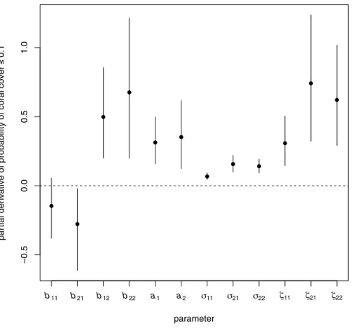
Figure 6 Elements of the gradient vector of partial derivatives of the long-term probability of coral cover less than or equal to 0.1 with respect to elements of the B matrix (effects of transformed composi-tion in a given year on transformed composicomposi-tion in the following year), the a vector (overall intercept, representing among-site mean proportional changes in transformed composition at the origin), the co-variance matrix of random temporal variation6, and the covariance matrix of among-site variability Z. For each parameter, the dot is the posterior mean and the bar is a 95% highest posterior density cred-ible interval. For the covariance matrices, the elementsσ12andζ12are not shown, because they are
con-strained to be equal toσ21andζ21respectively. The horizontal dashed line is at zero, the no-effect value.
Which model parameters have the largest effects on the probability of low coral cover?
Both among-site variability and internal dynamics, particularly of other relative to algae and coral (component 2), were important in determining the probabilityq0.1 of coral
cover≤0.1 in the region.Figure 6shows the direction in parameter space along which the probability of low coral cover will reduce most rapidly (the estimated gradient vector ofq0.1with respect to all the model parameters). The four parameters to whichq0.1was
most sensitive were (in descending order:Fig. 6)ζ21 (among-site covariance between
transformed components 1 and 2),b22(effect of component 2 on next year’s component
2),ζ22(among-site variance of component 2), andb12(effect of component 2 on next year’s
component 1). Although there was substantial variability among Monte Carlo iterations in the values of these derivatives, the rank order of magnitudes was fairly consistent (Fig. A41). All four most important parameters had positive effects onq0.1(Fig. 6), so reducing these
of low coral cover were relatively unimportant (Fig. 6, derivatives ofq0.1with respect to
σ11,σ21 andσ22 all had posterior means close to zero). The signs of the effects of each
parameter onq0.1, sensitivities for coral cover thresholds 0.05 and 0.2, and elasticities, are
discussed further inSections A15andA16.
How informative is a snapshot about long-term site properties? For both components of transformed composition, a snapshot of reef composition at a single time on a randomly-chosen site will be informative about the stationary mean (correlations between true value at a given time and stationary mean: component 1 posterior mean 0.84, 95% HPD interval (0.75,0.91); component 2 posterior mean 0.82, 95% HPD interval (0.73,0.90)). This is consistent with the negative relationship between long-term probability of coral cover≤0.1 and observed mean coral cover (Fig. 5). Thus, while long-term monitoring of East African coral reefs is important for other reasons, it should be possible to identify those with high conservation value (in terms of benthic composition) from a single survey.
DISCUSSION
In the long term (as t→ ∞), among-site variability dominated within-site temporal variability in East African coral reefs. In consequence, the long-term probability of coral cover≤0.1 varied substantially among sites. This suggests that it is in principle possible to make reliable decisions about the conservation value of individual sites based on a survey of multiple sites at one point in time, and to design conservation strategies at the site level. This was not the only possible outcome: if within-site temporal variability dominated among-site variability, among-site differences would be neither important nor predictable in the long term.
In our study, the sites with the highest long-term conservation value are those with very low long-term probabilities of coral cover≤0.1 (Fig. 5), a threshold chosen based on evidence that coral cover≤0.1 is detrimental to reef function (Kennedy et al., 2013;Perry et
al., 2013;Perry et al., 2015;Roff, Zhao & Mumby, 2015). Many of these sites are Tanzanian patch reefs, which may have maintained high coral cover despite disturbance because of local hydrography (McClanahan et al., 2007b), and are priority sites for conservation, with high alpha and beta diversity (Ateweberhan & McClanahan, 2016). Thus, it seems likely that sites of high conservation value based on community dynamics may also be sites of high diversity resulting from a combination of physical factors and biological interactions (Huston, 1985;West & Salm, 2003). However, the absence of strong spatial autocorrelation in long-term probabilities of coral cover≤0.1 suggests that it will be necessary to consider conservation value at small spatial scales, rather than simply to identify subregions with high conservation value. Similarly,Vercelloni et al. (2014)found that trajectories of coral cover on the Great Barrier Reef were consistent at the scale of km2, but not at larger spatial scales. They argued that it would therefore be appropriate to focus management actions at the km2scale. Also, it may be easier to persuade local communities to accept management at such scales than at larger scales (McClanahan, Muthiga & Abunge, 2016).
In this study, we aggregated all scleractinians and Milleporainto a single category. Comparisons between models with this level of aggregation and models in which corals are separated into functional groups show that aggregation can hide important biological differences (e.g. Clancy et al., 2010). These differences can lead to reefs dominated by different coral taxa having very different dynamics. For example, in models of reefs in the US Virgin Islands, two sites dominated by long-livedOrbicellashowed less year-to-year variability than a site dominated by short-lived species (Gross & Edmunds, 2015). These differences will affect management priorities. For example, in the Western Indian Ocean, sites which experienced a large number of Degree Heating Weeks during the 1998 bleaching event tended to show relative decreases in bleaching-susceptible genera such asAcropora andMontipora, and relative increases in resistant genera such asPorites(McClanahan et al.,
2007a). Priority sites might be those in which coral diversity has been maintained through
acclimation (McClanahan et al., 2007b), or in which rare and susceptible genera have survived (McClanahan et al., 2007a). Clearly, statistical models of coral dynamics would be more useful for management if they had higher taxonomic resolution. However, the number of parameters required is roughly proportional to the square of the number of taxa, except in special cases where corals are sufficiently rare that most of the interactions among taxa can be ignored (Gross & Edmunds, 2015). Separating corals into a small number of groups based on life-history strategies (Darling et al., 2012) may be the best balance between taxonomic resolution and model complexity.
spatial autocorrelation in the probability of low coral cover (Section A10 andFig. A40) suggests that connectivity is relatively unimportant for our analysis, it is possible that either current patterns of connectivity or future changes in these patterns may affect both the interpretation of stationary distributions and the optimal management strategy.
In conclusion, our analysis extends the broadly-applicable vector autoregressive approach to community dynamics (reviewed by Hampton et al., 2013) by quantifying random among-site variability in dynamics. This gives a new perspective on the long-term behaviour of the set of communities in a region, as a set of stationary distributions with random but persistent differences. The extent of these differences relative to temporal variability determines how predictable the behaviour of individual sites will be. Since these differences may be associated with differences in conservation value, probabilistic risk assessment based on this approach can be used to suggest conservation strategies at both site and regional scales. At site scales, our approach can be used to identify potential coral refugia, while at regional scales, it can identify the parameters with most influence on conservation objectives.
ACKNOWLEDGEMENTS
We are very grateful to Peter Mumby, four other anonymous reviewers and the editor for suggesting improvements to the manuscript.
ADDITIONAL INFORMATION AND DECLARATIONS
Funding
This work was supported by NERC grant NE/K00297X/1. The funders had no role in study design, data collection and analysis, decision to publish, or preparation of the manuscript.
Grant Disclosures
The following grant information was disclosed by the authors: NERC: NE/K00297X/1.
Competing Interests
John F. Bruno is an Academic Editor for PeerJ. Tim McClanahan is an employee of the Wildlife Conservation Society.
Author Contributions
• Katherine A. Allen, Fiona Chong and Matthew Spencer conceived and designed the experiments, analyzed the data, contributed reagents/materials/analysis tools, wrote the paper, prepared figures and/or tables, reviewed drafts of the paper.
• John F. Bruno conceived and designed the experiments, wrote the paper, reviewed drafts of the paper.
• Tim R. McClanahan conceived and designed the experiments, performed the experiments, wrote the paper, reviewed drafts of the paper.
Supplemental Information
Supplemental information for this article can be found online athttp://dx.doi.org/10.7717/ peerj.3290#supplemental-information.
REFERENCES
Aitchison J. 1986.The statistical analysis of compositional data. London: Chapman and
Hall.
Aitchison J. 1989.Measures of location for compositional data sets.Mathematical
Geology21:787–790 DOI 10.1007/BF00893322.
Ateweberhan M, McClanahan TR. 2016.Partitioning scleractinian coral diversity
across reef sites and regions in the Western Indian Ocean.Ecosphere7(5):01243 DOI 10.1002/ecs2.1243.
Baker AC, Glynn PW, Riegl B. 2008.Climate change and coral reef bleaching: an
ecological assessment of long-term impacts, recovery trends and future outlook. Estuarine, Coastal and Shelf Science80:435–471DOI 10.1016/j.ecss.2008.09.003.
Bjørnstad ON, Falck W. 2001.Nonparametric spatial covariance functions: estimation
and testing.Environmental and Ecological Statistics8:53–70 DOI 10.1023/A:1009601932481.
Brook BW, O’Grady JJ, Chapman AP, Burgman MA, Ak¸cakaya HR, Frankham R. 2000.
Predictive accuracy of population viability analysis in conservation biology.Nature
404:385–387DOI 10.1038/35006050.
Bruno JF, Sweatman H, Precht WF, Selig ER, Schutte VGW. 2009.Assessing evidence
of phase shifts from coral to macroalgal dominance on coral reefs.Ecology
90(6):1478–1484DOI 10.1890/08-1781.1.
Carreiro-Silva M, McClanahan TR. 2012.Macrobioerosion of dead branchingPorites,
4 and 6 years after coral mass mortality.Marine Ecology Progress Series458:103–122 DOI 10.3354/meps09726.
Caswell H. 2001.Matrix population models: construction, analysis, and interpretation.
Second edition. Sunderland: Sinauer.
Chong F. 2016.The dynamics of East African coral reefs. B.Sc. dissertation, School of
Environmental Sciences, University of Liverpool, Liverpool.
Cinner JE, McClanahan TR. 2015.A sea change on the African coast? Preliminary social
and ecological outcomes of a governance transformation in Kenyan fisheries.Global Environmental Change30:133–139DOI 10.1016/j.gloenvcha.2014.10.003.
Clancy D, Tanner JE, McWilliam S, Spencer M. 2010.Quantifying parameter
uncer-tainty in a coral reef model using Metropolis-Coupled Markov Chain Monte Carlo. Ecological Modelling 221:1337–1347DOI 10.1016/j.ecolmodel.2010.02.001.
Connell JH. 1997.Disturbance and recovery of coral assemblages.Coral Reefs
Connell JH, Hughes TP, Wallace CC. 1997.A 30-year study of coral abundance, recruit-ment, and disturbance at several scales in space and time.Ecological Monographs
67(4):461–488DOI 10.1890/0012-9615(1997)067[0461:AYSOCA]2.0.CO;2.
Cooper JK, Spencer M, Bruno JF. 2015.Stochastic dynamics of a warmer Great Barrier
Reef.Ecology96:1802–1811DOI 10.1890/14-0112.1.
Darling ES, Alvarez-Filip L, Oliver TA, McClanahan TR, Coté IM. 2012.Evaluating
life-history strategies of reef corals from species traits.Ecology Letters15:1378–1386 DOI 10.1111/j.1461-0248.2012.01861.x.
De’ath G, Fabricius KE, Sweatman H, Puotinen M. 2012.The 27-year decline of
coral cover on the Great Barrier Reef and its causes.Proceedings of the National Academy of Sciences of the United States of America109:17995–17999
DOI 10.1073/pnas.1208909109.
Diamond J. 1986. Overview: laboratory experiments, field experiments, and natural
experiments. In: Diamond J, Case TJ, eds.Community ecology. New York: Harper & Row, 3–22.
Driver CC, Oud JHL, Voelkle MC. 2016.Continuous time structural equation modelling
with R packagectsem.Journal of Statistical SoftwareIn Press.
Egozcue JJ, Pawlowsky-Glahn V, Mateu-Figueras G, Barceló-Vidal C. 2003.Isometric
logratio transformations for compositional data analysis.Mathematical Geology
35(3):279–300DOI 10.1023/A:1023818214614.
Ginzburg LR, Slobodkin LB, Johnson K, Bindman AG. 1982.Quasiextinction
prob-abilities as a measure of impact on population growth.Risk Analysis21:171–181 DOI 10.1111/j.1539-6924.1982.tb01379.x.
Gorrostieta C, Ombao H, Bédard P, Sanes JN. 2012.Investigating brain connectivity
using mixed effects vector autoregressive models.NeuroImage59:3347–3355 DOI 10.1016/j.neuroimage.2011.08.115.
Gross K, Edmunds PJ. 2015.Stability of Caribbean coral communities quantified
by long-term monitoring and autoregression models.Ecology 96:1812–1822 DOI 10.1890/14-0941.1.
Hampton SE, Holmes EE, Scheef LP, Scheuerell MD, Katz SL, Pendleton DE, Ward
EJ. 2013.Quantifying effects of abiotic and biotic drivers on community dynamics
with multivariate autoregressive (MAR) models.Ecology94(12):2663–2669 DOI 10.1890/13-0996.1.
Hoffman MD, Gelman A. 2014.The No-U-Turn Sampler: adaptively setting path lengths
in Hamiltonian Monte Carlo.Journal of Machine Learning Research15:1351–1381.
Huston M. 1985.Patterns of species diversity on coral reefs.Annual Review of Ecology and
Systematics16:149–177DOI 10.1146/annurev.es.16.110185.001053.
Hyndman RJ. 1996.Computing and graphing highest density regions.The American
Statistician50(2):120–126DOI 10.2307/2684423.
Ives AR, Dennis B, Cottingham KL, Carpenter SR. 2003.Estimating community
stability and ecological interactions from time-series data.Ecological Monographs
Kaiser L. 1983.Unbiased estimation in line-intercept sampling.Biometrics39(4):965–976 DOI 10.2307/2531331.
Kennedy EV, Perry CT, Halloran PR, Iglesias-Prieto R, Schönberg CHL, Wissah M,
Form AU, Carricart-Ganivet JP, Fine M, Eakin CM, Mumby PJ. 2013.Avoiding
coral reef functional collapse requires local and global action.Current Biology
23:912–918DOI 10.1016/j.cub.2013.04.020.
Kenward MG. 1979.An intuitive approach to the MANOVA test criteria.Journal of the
Royal Statistical Society Series D28(3):193–198DOI 10.2307/2987868.
Keppel G, Van Niel KP, Wardell-Johnson GW, Yates CJ, Byrne M, Mucina L, Schut
AGT, Hopper SD, Franklin SE. 2012.Refugia: identifying and understanding safe
havens for biodiversity under climate change.Global Ecology and Biogeography
21:393–404DOI 10.1111/j.1466-8238.2011.00686.x.
Lange KL, Little RJA, Taylor JMG. 1989.Robust statistical modeling using the
t distribution.Journal of the American Statistical Association84:881–896 DOI 10.2307/2290063.
Lewis JB. 1989.The ecology ofMillepora.Coral Reefs8:99–107 DOI 10.1007/BF00338264.
Lindegren M, Möllmann C, Nielsen A, Stenseth NC. 2009.Preventing the collapse
of the Baltic cod stock through an ecosystem-based management approach. Proceedings of the National Academy of Sciences of the United States of America
106(34):14722–14727DOI 10.1073/pnas.0906620106.
Lütkepohl H. 1993.Introduction to multiple time series analysis. 2nd edition. Berlin:
Springer-Verlag.
Magnus JR, Neudecker H. 2007.Matrix differential calculus with applications in statistics
and econometrics. Third edition. Chichester: John Wiley & Sons.
Mateu-Figueras G, Pawlowsky-Glahn V, Egozcue JJ. 2011. The principle of working on
coordinates. In: Pawlowsky-Glahn V, Buccianti A, eds.Compositional data analysis: theory and applications. Chichester: John Wiley & Sons, 31–42.
McClanahan TR, Arthur R. 2001.The effect of marine reserves and habitat on
pop-ulations of East African coral reef fishes.Ecological Applications11(2):559–569 DOI 10.1890/1051-0761(2001)011[0559:TEOMRA]2.0.CO;2.
McClanahan TR, Ateweberhan M, Graham NAJ, Wilson SK, Ruiz Sebastián C,
Guillaume MM, Bruggemann JH. 2007a.Western Indian Ocean coral communities:
bleaching responses and susceptibility to extinction.Marine Ecology Progress Series
337:1–13DOI 10.3354/meps337001.
McClanahan TR, Ateweberhan M, Muhando CA, Maina J, Mohammed MS. 2007b.
Effects of climate and seawater temperature variation on coral bleaching and mortality.Ecological Monographs77(4):503–525DOI 10.1890/06-1182.1.
McClanahan TR, Muthiga NA, Abunge CA. 2016.Establishment of community
managed fisheries’ closures in Kenya: early evolution of the tengefu movement. Coastal Management 44:1–20DOI 10.1080/08920753.2016.1116667.
McClanahan TR, Muthiga NA, Mangi S. 2001.Coral and algal changes after the 1998
Mumby PJ, Hastings A, Edwards HJ. 2007.Thresholds and the resilience of Caribbean coral reefs.Nature450:98–101DOI 10.1038/nature06252.
Mutshinda CM, O’Hara RB, Woiwod IP. 2009.What drives community dynamics?
Proceedings of the Royal Society of London Series B: Biological Sciences276:2923–2929 DOI 10.1098/rspb.2009.0523.
Perry CT, Murphy GN, Graham NAJ, Wilson SK, Januchowski-Hartley FA, East HK.
2015.Remote coral reefs can sustain high growth potential and may match future
sea-level trends.Scientific Reports5:18289DOI 10.1038/srep18289.
Perry CT, Murphy GN, Kench PS, Smithers SG, Edinger EN, Steneck RS, Mumby PJ.
2013.Caribbean-wide decline in carbonate production threatens coral reef growth.
Nature Communications4:Article 1402DOI 10.1038/ncomms2409.
R Core Team. 2015.R: a language and environment for statistical computing. Vienna: R
Foundation for Statistical Computing.Available athttps:// www.R-project.org/.
Roff G, Zhao J-X, Mumby PJ. 2015.Decadal-scale rates of reef erosion following
El Niño-related mass coral mortality.Global Change Biology 21:4415–4424 DOI 10.1111/gcb.13006.
Sandin SA, Smith JE, DeMartini EE, Dinsdale EA, Donner SD, Friedlander AM, Konotchick T, Malay M, Maragos JE, Obura D, Pantos O, Paulay G, Richie M, Rohwer F, Schroeder RE, Walsh S, Jackson JBC, Knowlton N, Sala E. 2008.
Baselines and degradation of coral reefs in the Northern Line Islands.PLOS ONE
3(2):e1548DOI 10.1371/journal.pone.0001548.
Stan Development Team. 2015.Stan: a C++ library for probability and sampling.
Version 2.7.0.Available athttp:// mc-stan.org/.
Vercelloni J, Caley MJ, Kayal M, Low-Choy S, Mengersen K. 2014.Understanding
uncertainties in non-linear population trajectories: a Bayesian semi-parametric hi-erarchical approach to large-scale surveys of coral cover.PLOS ONE9(11):e110968 DOI 10.1371/journal.pone.0110968.
West JM, Salm RV. 2003.Resistance and resilience to coral bleaching: implications for
coral reef conservation and management.Conservation Biology 17(4):956–967 DOI 10.1046/j.1523-1739.2003.02055.x.
Żychaluk K, Bruno JF, Clancy D, McClanahan TR, Spencer M. 2012.Data-driven