Sharif University of Technology
Scientia IranicaTransactions E: Industrial Engineering http://scientiairanica.sharif.edu
Integrated bi-objective project selection and scheduling
using Bayesian networks: A risk-based approach
A. Namazian
, S. Haji Yakhchali, and M. Rabbani
Department of Industrial Engineering, College of Engineering, University of Tehran, Tehran, P.O. Box 14155-6619, Iran. Received 11 March 2017; received in revised form 4 February 2018; accepted 16 July 2018
KEYWORDS Project selection and scheduling;
Risk analysis; Bayesian networks; Multi-objective programming; Genetic algorithm.
Abstract. This paper presents a novel formulation for the integrated bi-objective problem of project selection and scheduling. The rst objective was to minimize the aggregated risk by evaluating the expected value of schedule delay and the second objective was to maximize the achieved benet. To evaluate the expected aggregated impacts of risks, an objective function based on the Bayesian Networks was proposed. In the extant mathematical models of the joint problem of project selection and scheduling, projects are selected and scheduled without considering the risk network of the projects indicating the individual and interaction eects of risks impressing the duration of the activities. To solve the model, two solution approaches were developed, one exact and one metaheuristic approach. Goal Programming (GP) method was adopted to optimally select and schedule projects. Since the problem was NP-hard (Non-deterministic Polynomial-time), an algorithm combining GP method and Genetic Algorithm (GA) was proposed, hence named GPGA. Finally, the eciency of the proposed algorithm was assessed not only based on small-size instances, but also by generating and testing representative datasets of larger instances. The results of the computational experiments indicated that it had acceptable performance in handling large-size and more realistic problems.
© 2019 Sharif University of Technology. All rights reserved.
1. Introduction
The permanence of organizations depends on their ability to select and implement right projects for adjusting to the competitive business environment. Thus, managers are faced with the problem of project portfolio selection and scheduling. Project portfolio selection, as a complicated decision-making process, is the procedure of evaluating individual projects and choosing a subset of them to implement so that
*. Corresponding author.
E-mail addresses: [email protected] (A. Namazian); [email protected] (S. Haji Yakhchali); [email protected] (M. Rabbani)
doi: 10.24200/sci.2019.21387
objectives of the organization will be satised. The complexity of the project selection problem is due to the high number of scenarios from which a subset (portfolio) of projects has to be chosen. After selecting a portfolio of projects, each enterprise requires to schedule them. Project scheduling consists in nding feasible start times for the activities of the projects such that the predened objectives are optimized without violating existing precedence or resource constraints. In the recent decades, project selection and scheduling problem has received signicant attention and various methods have been developed for solving it.
Models of project portfolio selection problem can be categorized in two main groups including Multi-Criteria Decision Making (MCDM) approaches for ranking the projects and mathematical programming models. Tuli et al. [1] introduced a decision-making
model of multi-criteria optimization for the project selection problem. For this purpose, they combined the soft set theory and analytic hierarchical model under fuzziness. The proposed decision support strategy was useful for the project managers to take decision in the perspective environment. Rathi et al. [2] developed a project selection approach based on a combination of fuzzy and Multi Attribute Decision Making (MADM) techniques in order to determine proper Six Sigma projects in automotive companies. The weights of evaluation criteria were obtained using the Modied Digital Logic (MDL) method and nal ranking was calculated by the primacy index obtained using fuzzy based VIKOR and Technique for Order of Preference by Similarity to Ideal Solution (TOPSIS) methodolo-gies. Besides the MCDM approaches, mathematical programming is widely used for the project selection problem. The selection is a function of maximization or minimization of the objectives and satisfaction of the resource constraints. Linear Optimization (LO), Integer Linear Programming (ILP), Goal Program-ming (GP), and Integer Goal ProgramProgram-ming (IGP) are more applicable mathematical optimization methods to project selection [3]. Some studies have used these methods for the project selection problem. Namazian and Haji Yakhchali [4] developed a project portfolio selection problem based on the schedule of the projects so that the minimum expected prot would be met in the shortest possible time period. In their research, because of their uncertain nature, durations of the activities were considered as semi-trapezoidal fuzzy numbers. Ultimately, they formulated the mentioned problem as a fuzzy linear programming model. Badri et al. [5] proposed a GP model for project portfolio selection in the information system projects. Arratia et al. [6] proposed a mathematical model framework for R&D project portfolio selection in which each project proposal comprised tasks with a specic type of expense. Their Mixed Integer Linear Programming (MILP) model framework handled dependencies within tasks as well as the eects of such dependencies.
Also, some scholars have used the combination of the mentioned approaches to dealing with the project selection problem. Tavana et al. [7] proposed a three-stage hybrid method for selecting an optimal combi-nation of projects. The proposed model comprised three stages and each stage was composed of several procedures. They used Data Envelopment Analysis (DEA) for the initial screening, TOPSIS for ranking the projects, and linear Integer Programming (IP) for selecting the most suitable project portfolio. Fatemeh and Sameh Monir [8] proposed a new model for project selection using the joint approach of Analytic Hierarchy Process (AHP) and Linear Programming (LP). AHP was used rst to perform the pair-wise comparisons among the selection criteria and later, to compare the
available projects against these criteria. The overall weight for each project was calculated and used as a coecient in the LP model.
In addition to project selection, the problem of project scheduling has attracted the attention of many researchers. Kellenbrink and Helber [9] analyzed the problem of project scheduling with a exible structure in which the activities were not completely known in advance. They presented a Genetic Algorithm (GA) to solve this type of scheduling problem and evaluated it in an extensive numerical study. Ji and Yao [10] studied a type of project scheduling problem in which durations and resource allocation times of the activities were considered as uncertain variables. They designed an uncertain programming model with the aim of minimizing the total cost and the overtime of the project under the constraints of time windows for allocating loans and the mid-term inspection. In their research, GA was employed to solve the proposed uncertain project scheduling model.
Also, the joint problem of project selection and scheduling has recently been addressed to simulta-neously select and schedule projects. Toghian and Naderi [11] developed a mixed integer linear mathemat-ical model for the integrated multi-objective problem of project selection and scheduling. The objectives were to optimize both total expected benet and resource usage variation. The problem of project selection and scheduling is of the NP-hard type [12]. Therefore, in recent years, meta-heuristic algorithms such as GA and colony algorithms have been proposed to solve them [13-20].
On the other hand, various methods have been developed for assessing risk in projects. For example, MCDM [21-27], Failure Mode and Eects Analysis (FMEA) [28-30], Fault Tree Analysis (FTA) [31-34], Monte Carlo Simulation (MCS) [35,36], and Bayesian Networks [37-40] are widely used to assess the risk of projects.
In the literature, the problems of project selection and scheduling, and project risk assessment have been separately investigated, and projects have been selected and scheduled without considering their risk networks. Risk network indicates the individual and interaction eects of risks within and among the projects. In prac-tical cases, projects may aect each other negatively duo to extant interactions among their risks. Since these interactions aect the duration and cost of the activities, they have a decisive role in project selection and scheduling problem. The failure to consider the eects of risks is one of the most important factors that leads to partial completion of the projects. As an example, the occurrence of a risk in one project may intensify the probability or impact of another risk in another project. To the best of our knowledge, these practical cases have not been considered in the project
selection and scheduling problem. In this context, Bayesian networks method can be used to model these interactions. In this paper, a new formulation for the integrated bi-objective problem of project selection and scheduling is proposed in which the undesirable eects of the risks of projects and their interactions are modeled by the application of Bayesian networks approach.
The problem can be described as follows. Suppose a set of projects are available in which each project has a certain duration. In each time period, each project extricates a certain benet after its completion time. There is also a risk network stating the potential risks and interactions among them in projects. The objective is to select a subset of projects by which the aggregated risk is minimized and the total benet is maximized. These two objectives are in conict with each other. On the one hand, regardless of the budget or resource constraint, maximizing the earned benet is intended by taking as many projects as available. On the other hand, selecting more projects leads to higher risk, which can reduce the benet. To solve the problem, two exact and metaheuristic approaches are presented. First, GP method as one of the multi-objective approaches is used to achieve optimal solution. Then, due to NP-hard structure of the problem, an algorithm combining GP and GA (GPGA) is proposed to cope with more realistic large-size problems. The rest of the paper is organized as follows. In Section 2, the Bayesian belief network approach is introduced. In Section 3, the formulation developed for the problem of project selection and scheduling is presented. Section 4 presents the pro-posed GPGA solution method for solving the model. In Section 5, as an illustration, the developed model is applied to a small-size instance. In Section 6, the eciency of the developed approach is assessed by generating large-size instances and nally, the paper is concluded in Section 7.
2. Bayesian networks
Bayesian networks, also called causal networks or Bayesian belief networks, are graphical representations of knowledge for reasoning under uncertainty and provide a good tool for decision analysis, including prior analysis, posterior analysis, and pre-posterior analysis [41]. Bayesian network is a general modelling approach, oering a compact presentation of the in-teractions in a stochastic system by visualizing system variables and their dependencies [42]. The Bayesian formula is the basis of the Bayesian network method. It reects the interrelation between the prior probability and posterior probability and can use existing prior probability to derive the specic probability of an accident. This approach is widely used in uncertainty
analysis [43]. For n mutually exclusive hypotheses (j = 1; 2; :::; n), Bayes' theorem is represented by the following relationship:
P (HjjE) = PnP (EjHj) P (Hj) i=1P (EjHi) P (Hi)
;
where P (HjjE) is the posterior or conditional
proba-bility for the hypothesis H (j = 1; 2; :::; n) based on the obtained evidence (E), P (Hj) denotes the prior
probability, P (EjHj) represents conditional
probabil-ity assuming that Hj is true, and the denominator
represents the total probability, which is a constant value [44]. A Bayesian network consists of two main parts: a qualitative part and a quantitative part. The qualitative part is a Directed Acyclic Graph (DAG) in which the nodes reect the system variables and the edges of the graph represent the conditional de-pendences between variables. The quantitative part is a set of conditional probability functions, stating the relations between the nodes of the graph [42]. The nodes that are the starting ones and do not have an inward arrow are called the parent nodes. The other nodes, which have inward arrows connected to them, are the child nodes. In order to run the calculations, it is necessary to dene the states and probabilities for each node [45]. Considering the conditional de-pendencies of variables, Bayesian network represents the joint probability distribution, P (U), of variables U = fA1; :::; Ang, as:
P (U) =Yn
i=1
P (AijP a (Ai));
where P a(Ai) is the parent set of variables Ai.
Accord-ingly, the probability of Ai is calculated as:
P (Ai) =
X
UnAi
P (U);
where the summation is taken over all the variables except for Ai.
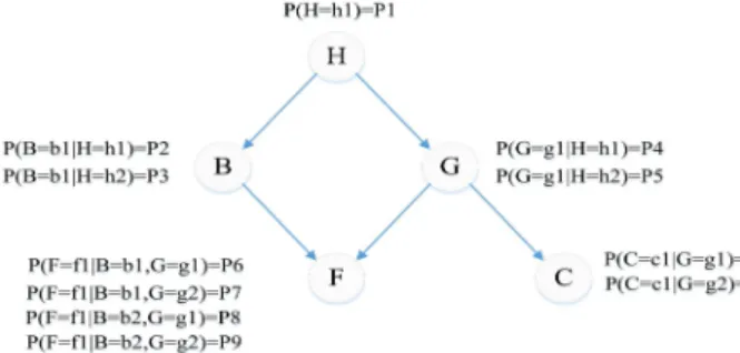
Figure 1 is an illustration of a simple Bayesian network. This network consists of 5 binary variables in
which the arrows (directed links) going from one vari-able to another reect the relations between varivari-ables. In this example, the arrow from B to F means that B has a direct inuence on F and thus, the value of F depends on the value of B. Prior probability and condi-tional probabilities of variables are shown in Figure 1. Based on Figure 1, Bayesian networks provide an appropriate structure for modeling dependencies among risks of the projects.
3. Mathematical model formulation
Most researches on project selection problem with the aim of minimizing risk have used MCDM approaches to modeling problems in which decision-making is carried out based only on risk probability and the consequences of risks are not taken into account. Furthermore, the interactions among risks, which can cause even greater consequences, have not been considered in the developed models. As mentioned before, the available mathematical models suer from serious shortcomings including the failure to consider risks and their interac-tions in the project selection and scheduling problem. This section presents a new formulation for the project portfolio selection and scheduling problem with the ob-jectives of minimizing the expected value of aggregated risk and maximizing the benets of the projects. The developed model is based on the Bayesian networks, in which consequences and interactions of risks are simultaneously considered.
Suppose we have N projects for which each project j has njactivities and nrjrisks. To perform the
activity r of project j, its initially estimated duration is d0
rj in which the eects of extant risks are not
considered. By applying the respective eects of risks, its actual duration will be drj. The notation used to
formulate the model is as follows:
Indices
j; l Project index r Activity index k Risk index t Time index
Parameters and decision variables Rpor Project portfolio risk
Rkj The risk k of project j
PP or Bayesian-based probability function of
risks of the project portfolio RT0
rlkj Initial time impact of risk k of project
j on activity r of project l RT
rlkj Cumulative time impact of risk k of
project j on activity r of project l
P aI(R
kj) The set of internal parent risks of risk
k of project j P aEl(R
kj) The set of external parent risks of risk
k of project j from project l val(P aI(R
kj)) Takes the value of 1 in the event of
P aI(R
kj) and zero otherwise
val(P aEl(R
kj))Takes the value of 1 in the event of
P aEl(Rkj) and zero otherwise
/T
P aI(Rkj)) Percentage of increase in time impact
of risk k of project j in the event of P aI(R
kj)
/T
P aEl(Rkj)) Percentage of increase in time impact
of risk k of project j in the event of P aEl(Rkj)
Nkj The number of external projects the
risks of which aect risk k of project j Ukj The set of external projects the risks
of which aect risk k of project j Grl The set of risks that aect the activity
r of project l d0
rj The estimated duration of activity r of
project j
drj The actual duration of activity r of
project j
jn The last activity of project j
esrj The earliest start time of activity r of
project j
lsrj The latest start time of activity r of
project j
T Horizontal time period for implementing all projects (with index t)
T0 The time period after project
completion time that is protable (with index t0)
P re(r; r0; j) The predecessor relation between
activities r and r0 of project j
a Interest rate
bt0j The benet derived from project j
in the period of time t0 after project
completion
yj Takes the value of 1 if project j is
selected and zero otherwise
xrjt Takes the value of 1 if activity r of
project j at time t is performed and zero otherwise
To calculate the expected value of aggregated time risk resulting from the interactions among risks, its probability and impacts should be evaluated. The respective probability part of the expected value is
evaluated by the application of Bayesian networks in which the joint probability of risks is determined by considering the states of risks and their parent risks. Thus, the rst objective function is to minimize the expected value of project portfolio risk as shown in Eq. (1):
Min Z1=E RTP or
=X Rkj 0 @Y k;j
PP or
X r X l X k X j RT rlkj 1 A; (1) where PP or is calculated as follows:
PP or= P RkjjP aI(Rkj)yj
Y
v2Ukj
(1 yv)
+ X
l2Ukj
P RkjjP aI(Rkj) ; P aEl(Rkj)yjyl
Y
v2Ukjnl
(1 yv) +
X
l1;l22Ukj
P
RkjjP aI(Rkj) ;
P aEl1(R
kj) ; P aEl2(Rkj)
yjyl1yl2
Y
v2Ukjnl1;l2
(1 yv) + :::
+ X
l1;:::;lk2Ukj
P
RkjjP aI(Rkj) ; P aEl1(Rkj) ; :::;
P aElk(R
kj) yj Y v12l1;:::;lk yv1 Y
v22Ukjnl1;:::;lk
(1 yv2) + :::
+ X
l1;:::;lNkj2Ukj
P
RkjjP aI(Rkj) ; P aEl1(Rkj) ; :::;
P aElNkj(Rkj)
yj
Y
v12l1;:::;lNkj
yv1+ (1 yj) ; (2)
where RT
rlkj is calculated based on Eq. (3):
RT
rlkj = val (Rkj) yjRTrlkj0
1 + X
P a(Rkj)
val P aI(R
kj)TP aI(Rkj)
+valP aEl(Rkj)
T
P aEl(Rkj)yl
: (3)
According to Eq. (3), the respective time impacts are determined by regarding the initial and cumulative impacts of risks on the durations of the activities. The cumulative impacts of risks represent the total impact for each risk including the initial impact and intensifying impact caused by their parent risks.
The second objective function of the model is to maximize the benet of the selected projects as shown in Eq. (4):
Max Z2=
X j X t X t0 X jn
xrjt bt0j
(1 + a)t+drj+t0 1: (4)
Also, the constraints of the model are shown in Eqs. (5) to (10):
drj= d0rj
0
@1 + PP or
X
Rkj2Grl
RT rlkj
1
A 8r ; 8j; (5)
lsrj
X
t=esrj
xrjt= yj 8r ; 8j; (6)
esXrj 1
t=1
xrjt= 0 8r ; 8j; (7)
T
X
t=lsrj+1
xrjt= 0; 8r ; 8j; (8)
T
X
t=1
(t + drj) xrjt T
X
t=1
t xr0jt
8 (r; r0; j) 2 pre (r; r0; j) ; (9)
yj; xrjt= f0; 1g : (10)
Constraint (5) calculates the actual duration for each activity regarding the eective risks that may increase its duration. Constraint (6) indicates that activities of a project are scheduled if and only if the respective project is selected. According to Constraints (7) and (8), each activity is performed in its acceptable time interval. Constraint (9) shows the predecessor relation-ships between activities. Finally, the sign constraint corresponding to the decision variables of the model is mentioned in Constraint (10).
As can be seen, Eq. (2) is a nonlinear function in the form of multiplication of decision variables. If all decision variables are multiplied by each other, their projects have been selected to be placed in the project portfolio and the result of multiplication will be equal to one. Otherwise, at least one project is not selected and the multiplication will be equal to zero. As a
result, the multiplication of decision variables can be substituted with one new binary variable, y = n
i=1yi,
by applying the following inequalities:
y 1 + M
n
X
i=1
yi n
! ;
y n1
n
X
i=1
yi
! ;
in which M is a positive large number. In the worst case, for the problem with n projects, this model needs (2n 1) variables, all possible subsets of projects, and
2(2n n 1) constraints to linearize the multiplication
of binary variables. As a result, achieving the optimal solutions to large-size problems is not possible in a reasonable run time. In the next section, an approach is proposed to deal with this problem.
4. The proposed GPGA approach
In the present section, the proposed solution approach is presented. This approach has two steps. In the rst step, the GP method is used to transfer the bi-objective model to a single-bi-objective structure. Then, in the second step, GA is applied to obtaining the near-optimal solution to the problem.
4.1. GP method
The GP developed to deal with multi-objective decision-making problems is a mathematical program-ming approach to assigning optimal values to a set of variables in problems with multiple, conicting objectives, among which there are measures of priority. This method allows one to take into account many objectives, simultaneously, while decision-making seeks the best solution among a set of feasible solutions [46]. It attempts to minimize the deviations between the desired goals and the realized results. Furthermore, these goals should be scaled based on their measure-ment methods. Deviation variables can be positive or negative. A positive deviation variable (d+) represents
over-achievement of the goal, while a negative deviation variable (d ) represents under-achievement of the goal. By utilizing these deviation variables, the general GP model can be stated as follows:
Min X
i
wipi d+i + di
;
Subject to : X
j
aijxj gi = d+i di ;
where wi is the weight of goal i, pi is the priority
of goal i, aij is the technological coecient between
decision variable i and constraint j, xj is decision
variable i, d+
i is the positive deviation variable i, di is
the negative deviation variable i, and gi is the desired
value for goal i.
4.2. Problem formulation as a GP model To formulate the mathematical model as a GP model, the objectives and constraints are stated in the following:
Risk-related objective: The aggregated risk re-sulting from the selected projects is evaluated based on the risk-related objective. According to Eq. (1), the respective equation is formulated as Eq. (11):
Risk objective function gr= d+r dr: (11)
gris the threshold of risk acceptability of the
orga-nization. It should be noted that the variable can also be set to zero if the desired value is not known.
Benet-related objective: The benet-related objective, which is to be maximized, represents the total benet derived from the implemented projects. As mentioned earlier, bt0j is the benet derived from
implementing project j at period of time t0 after
project completion time. According to Eq. (4), the respective equation in GP terms is formulated as:
Benet objective function gb= d+b db: (12)
gb is the maximum anticipated benet resulting
from the selected projects.
The objective function: The objective function attempts to minimize the sum of the deviations associated with the constraints in the model.
Min = w1 d+r + dr
+ w2 d+b + db
: (13) In addition to Constraints (11) and (12), the other constraints of the model are Constraints (5) to (10). 4.3. GA structure
GA, motivated by the natural evolution process, is a robust algorithm which can be used to solve search and optimization problems. In a simple GA, rst, a suitable encoding or representation of the problem should be devised. Then, a set of possible solutions treated as the population is produced through a ran-dom process. Afterwards, a tness value is calculated for each solution in the population and then, the solutions are ranked based on their tness values. Each solution has a chance to be selected according to its tness value to the problem. Better solutions have higher probabilities of being selected to reproduce ospring. The individuals, during the reproduction phase, are selected from the population and recombined to produce ospring as the next generation. On the basis of a selection mechanism, a set of chromosomes is chosen for crossover and mutation. This process is called generation. The generation is iterated until the stopping conditions are met.
4.3.1. Chromosome representation
Since two processes of project selection and scheduling have to be done simultaneously, a two-level encoding scheme is used to generate solution chromosomes; project selection in the rst level and project scheduling in the second level. After generating the initial popu-lation, crossover and mutation operators are applied to chromosomes in the rst level to produce ospring. Then, changed chromosomes are transferred to the second level for determining scheduling of the selected projects, to be aected again by the crossover and mutation operators.
For the rst level, a binary representation is used to determine the project selection process. For this purpose, a chromosome whose number of genes is as large as the number of projects is considered. Binary values are assigned to each gene for which values 1 and 0 represent the selection and non-selection of the project, respectively.
Figure 2 shows a sample chromosome for a prob-lem with 5 projects, illustrating selection of the projects 1, 2, and 5.
At the second level, for each project selected in the previous level, a chromosome is generated for which the number of genes is determined with regard to the number of activities in the respective project. A permutation of the activities can be considered as the initial solution chromosome. Since the precedence relationship between activities may not be satised by the generated chromosome, the validation process should be carried out on it. Algorithm 1 can be used to validate the initial chromosome.
According to Algorithm 1, starting from the left side, each member of the initial chromosome is transferred to the respective validated chromosome if and only if all of its predecessors have previously been assigned to the new chromosome. At each step, the gene (activity) selected to be transferred to the new chromosome is removed from the previous one and
Figure 2. Sample chromosome for the rst level.
Algorithm 1. Validation procedure for the initial chromo-some.
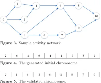
Figure 3. Sample activity network.
Figure 4. The generated initial chromosome.
Figure 5. The validated chromosome.
added to the new chromosome. This process continues until all members of the initial chromosome are as-signed to new chromosomes. For example, assume that a project with the activity network shown in Figure 3 is selected at the rst level (activities 0 and 10 are dummy).
Figure 4 illustrates an initial chromosome gen-erated by the permutation function of its number of activities. Based on the activity network stating the precedence relationship between activities and by applying Algorithm 1, the validated chromosome will be as given in Figure 5.
4.3.2. Fitness function and selection method
As mentioned before, GP method attempts to minimize deviations of the realized results from the desired goals. Thus, the tness function of GA is computed as:
Fitness = 1
w1 d+r + dr+ w2 d+b + db
:
Also, to select potentially useful solutions for recombi-nation, roulette wheel selection method is employed, in which a tness level is assigned to the solutions. This tness level is used to associate a probability of selection with each individual chromosome. The probability of selection is calculated for each individual as the ratio of its tness level to the cumulative tness of the whole population.
4.3.3. Crossover and mutation operators
In the proposed GA, due to the dierences in the encoding schemes for the rst level and the second level, various crossover and mutation operators are utilized to generate feasible ospring.
4.3.4. Crossover and mutation operators for the rst level (project selection)
Chromosomes in the rst level have binary values. Thus, in order to generate ospring, the following
Figure 6. Three-parent crossover operator.
crossover operator can be used. First, three parents are randomly selected. Each gene from the rst parent is compared with the same gene from the second parent. If they are the same, this gene is transferred to the ospring. If they are not the same, it is compared with one from another parent. In the case of similarity with the gene from the third parent, the gene from the rst parent and otherwise, the gene from the third parent is transferred to the ospring. This three-parent crossover operator is graphically illustrated in Figure 6. For mutation in the rst level, a simple binary mutation operator can be used. One gene from the parent is randomly selected and its values are replaced by another binary value.
4.3.5. Crossover and mutation operators for the second level (project scheduling)
To produce ospring from parents, the traditional crossover and mutation operators may generate infea-sible solutions in which some activities are duplicated or missing in the respective ospring. To avoid illegal ospring, the following genetic operators can be used. These operators generate feasible solutions in which activities are not duplicated or missing. After using these operators, Algorithm 1 should be applied to veri-fying the generated solutions regarding the precedence relationships between activities.
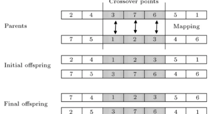
Partially Mapped Crossover (PMX). The PMX operator acts as a two-point crossover for sequence encoding through a repairing procedure. Having selected a pair of parents, the sequences of activities between two randomly specied positions are exchanged. The resulting ospring may not be feasible due to duplication of activities. Therefore, a mapping is established for the exchanged parts. Finally, a repairing procedure that replaces the repeated activities by their corresponding activities is applied to legalizing the ospring. The procedure of the PMX operator is illustrated in Figure 7.
Order Crossover (OX). The OX operator pro-duces ospring by transferring a subsequence of random length and position from one parent, and lling the remaining positions according to the order from the other parent. A subsequence between two random positions of a parent is transferred to one of the ospring in the same position. The activities
Figure 7. PMX operator.
Figure 8. OX operator.
Figure 9. IM operator.
that are already in the subsequence are removed from the second parent. The unselected activities in the second parent are then inserted into the empty positions of the ospring while preserving their original orders in the parent. This operator is shown in Figure 8.
Insert Mutation (IM). The IM operator ran-domly selects a position and inserts the activity in the position into another random point. The proce-dure of the IM operator is illustrated in Figure 9.
Swap Mutation (SM). The SM operator ran-domly selects two positions and then, swaps the activities in the positions as illustrated in Figure 10.
5. Numerical example
As an illustration of the developed model, a numerical example is presented in this section.
5.1. Sample problem
In the sample problem, as shown in Figure 11, a network consisting of three projects is considered in which each project contains seven activities. The network of these projects and durations of the activities
Figure 10. SM operator.
Figure 11. Network of the projects.
are shown in Figure 11. The benets of the projects in the time periods after project completion time are stated in Table 1. In this problem, the interest rate is assumed to be 0.1.
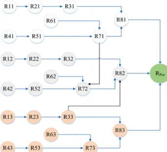
The supposed risk network of the projects, in-cluding the risks and their interactions, is shown in Figure 12.
Figure 12 indicates that in addition to the inter-actions among risks in each project, some risks from one project can aect the risks in other projects. For
Table 1. Benets of the projects. Time periods after project completion
time (t0)
1 2 3 4 5
Project
P1 14 16 20 24 29 P2 13 15 20 25 31 P3 12 17 23 27 33
Figure 12. Network of the risks.
example, risk R71 from project 1 has an impact on risk R72 of project 2. This means that in the case of selecting both projects 1 and 2, the occurrence of the risks in project 1 can increase the probabilities or consequences of risks in project 2. Furthermore, risks in each project, if selected, aect the project portfolio risk and may increase durations of activities of the respective project as well as activities of other projects. The predecessor relationships between activities as well as the earliest and latest times for each activity and their eective risk(s) are presented in Table 2. 5.2. Risk prior and conditional probability
assessment
Prior probability can be interpreted as the evaluated probability of a risk, which is not aected by other activated risks. On the other hand, conditional prob-ability can be interpreted as the evaluated probprob-ability of a risk, which is impressed by another risk inside the network. Qualitative scales are often used to express such probabilities with 5 to 10 levels. In this paper, we use the 5-level scale to present prior and conditional probabilities of risks as shown in Table 3.
5.3. Risk impact assessment
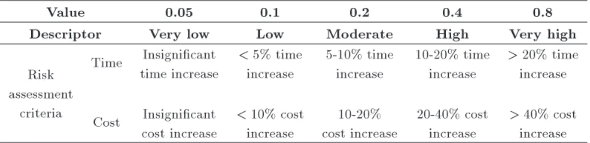
Impact or consequence refers to the extent to which a risk might aect the project. The main impact assessment criteria include time, cost, quality, and scope. In this paper, the time eects of risks are considered, although they can be generalized to cost factor. The assessment methods for time and cost eects of risks are shown in Table 4.
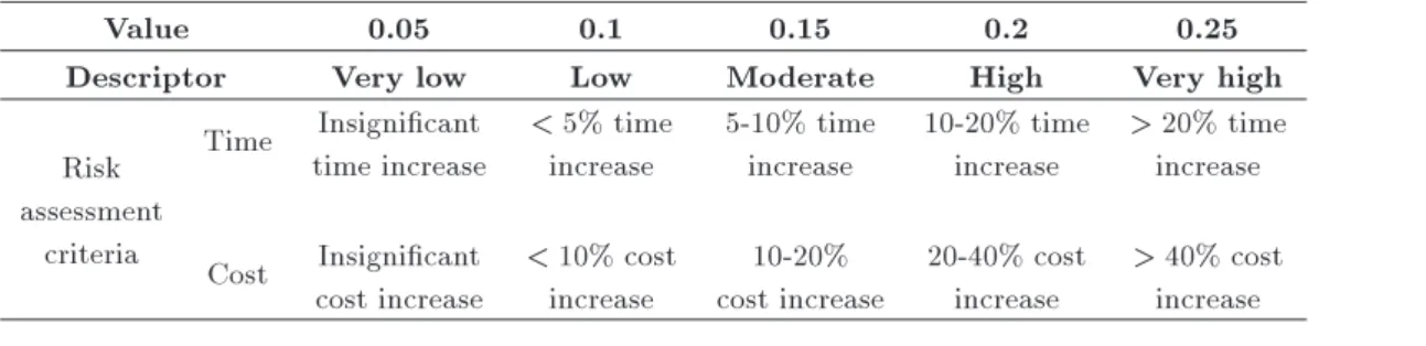
In addition to the independent eect of each risk on the project risk assessment criteria, the interactions among risks will amplify these eects. To assess the severity of the eects of risks on each other, we use the
Table 2. Predecessor relationships, start times, and nish times of the activities.
Activity 1 2 3 4 5 6 7
Predecessor(s) - 1 1 23 4 4 56
EST 0 2 2 5 7 7 11
EFT 2 3 5 7 10 11 13
LST 0 4 2 5 8 7 11
LFT 2 5 5 7 11 11 13
Eective risk(s) R11 R21
R31 R41 R51 R61 R71 R81
Activity 8 9 10 11 12 13 14
Predecessor(s) - 8 8 10 9 11 12
11 13
EST 0 3 3 5 8 8 12
EFT 3 7 5 8 11 12 14
LST 0 5 3 5 9 8 12
LFT 3 9 5 8 12 12 14
Eective risk(s) R12 R22 R32
R42 R52 R62 R72 R82
Activity 15 16 17 18 19 20 21
Predecessor(s) - 15 15 16 18 19 20
17
EST 0 1 1 4 7 9 13
EFT 1 3 4 7 9 13 14
LST 0 2 1 4 7 9 13
LFT 1 4 4 7 9 13 14
Eective risk(s) R13 R23
R33 R43 R53 R63 R73 R83
Table 3. Scales of prior and conditional probabilities.
Annual frequency Probability
Descriptor Denition Descriptor Value
Frequent Up to once in 1 month or more Very high 0.9 Likely Once in 1 month up to once in 6 months High 0.7 Possible Once in 6 months up to once in 18 months Medium 0.5 Unlikely Once in 18 months up to once in 30 months Low 0.3
Rare Once in 30 months or less Very low 0.1
Table 4. Time and cost impact assessment.
Value 0.05 0.1 0.2 0.4 0.8
Descriptor Very low Low Moderate High Very high
Risk assessment
criteria
Time Insignicant time increase
< 5% time increase
5-10% time increase
10-20% time increase
> 20% time increase Cost Insignicant
cost increase
< 10% cost increase
10-20% cost increase
20-40% cost increase
> 40% cost increase
Table 5. Interactive time and cost impact assessment.
Value 0.05 0.1 0.15 0.2 0.25
Descriptor Very low Low Moderate High Very high
Risk assessment
criteria
Time Insignicant time increase
< 5% time increase
5-10% time increase
10-20% time increase
> 20% time increase Cost Insignicant
cost increase
< 10% cost increase
10-20% cost increase
20-40% cost increase
> 40% cost increase
5-level scale, as shown in Table 5, for the assessment of impacts.
The values in the above table have been set so that the maximum change in the cumulative eects is equal to one.
5.4. Project portfolio risk assessment
Based on the identied risks and their relationships, the Bayesian networks-based model can be built using the software AgenaRisk. In a Bayesian network, for each variable (risk), the variable status as well as its table of prior and conditional probabilities should be determined. The status of each variable is determined based on its conditions during the projects. For exam-ple, the variable RPor (project portfolio schedule delay
risk) is assigned two states, namely `Low' and `High.' Thus, the remaining variables have two opposite states: `True' indicates occurrence of the risk and `False' indicates its non-occurrence. The assignments `Low' and `High' are dened as time-overrun durations, which are less than 15% and greater than 15% compared to the original schedule for completing the project portfolio, respectively. It should be noted that these computations can also be performed for cost-overrun expenditures compared to the original budgeting. How-ever, in this study, only the time criterion is discussed. Tables of prior and conditional probabilities for the variables `project portfolio schedule delay risk' (RP or) and R71, as an example, are shown in
Fig-ures 13 and 14, respectively.
Finally, the Bayesian networks-based model and evaluated probabilities for states of project portfolio risks are shown in Figure 15.
Figure 6 illustrates the model output for the project portfolio. It is estimated that the probability of schedule delay in the project portfolio is approximately 0.47 for the state of `Low,' whereas it is 0.53 for the state of `High.' As a result, the duration of the
Figure 14. Conditional probability table for the output variable `R71'.
project portfolio tends to get extended with time-overrun durations greater than 15% of the original duration.
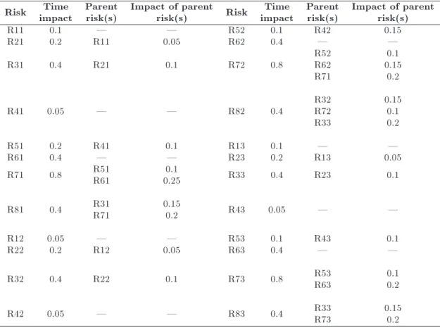
The consequences associated with individual risks and parent risks are stated in Table 6.
According to Table 6, for example, the individual time consequence of R71 is 0.8, and risks R51 and R61 are its parent risks. As a result, in a situation that R71 and at least one of its parent risks have occurred, the time consequence of R71 will be increased.
5.5. Model results
The results of problem formulation as a GP model are shown in Table 7.
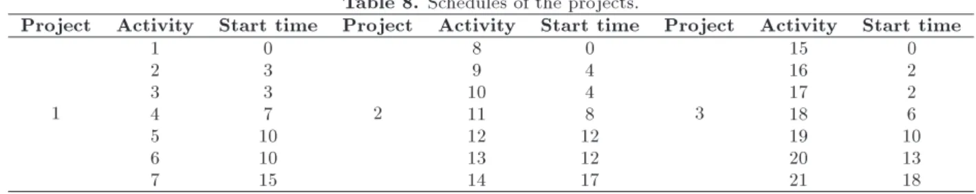
Table 7 illustrates the selected project(s) for dierent values of targets and weights of goals. As shown in this table, when the weight of the risk-related objective is increased, the optimal solution includes only project 2, whereas increasing the weight of the benet-related objective leads to selecting all the projects to be placed in the project portfolio. Consequently, the higher the value of the risk-related target, the greater the number of projects in the project portfolio. In other words, in the case that the threshold of risk acceptability of the organization is increased, more projects are selected to construct the project portfolio. In the case of selecting all projects (e.g. w1=w2 = 40, g1 = 1 and g2 = 70), each project is scheduled as shown in Table 8.
According to Table 8, activities can be started at their earliest start times. The durations of activities
Figure 15. Bayesian networks-based model and evaluated probabilities for the states of the variables. Table 6. The consequences of risks.
Risk impactTime Parentrisk(s) Impact of parentrisk(s) Risk impactTime Parentrisk(s) Impact of parentrisk(s)
R11 0.1 | | R52 0.1 R42 0.15
R21 0.2 R11 0.05 R62 0.4 | |
R31 0.4 R21 0.1 R72 0.8 R52R62
R71
0.1 0.15
0.2
R41 0.05 | | R82 0.4 R32R72
R33
0.15 0.1 0.2
R51 0.2 R41 0.1 R13 0.1 | |
R61 0.4 | | R23 0.2 R13 0.05
R71 0.8 R51R61 0.250.1 R33 0.4 R23 0.1
R81 0.4 R31R71 0.150.2 R43 0.05 | |
R12 0.05 | | R53 0.1 R43 0.1
R22 0.2 R12 0.05 R63 0.4 | |
R32 0.4 R22 0.1 R73 0.8 R53R63 0.10.2
Table 7. Optimal solutions for dierent targets and weights.
w1=w2 = 80 w1=w2 = 40 w1=w2 = 20
g1 g2 Selected project(s) g1 g2 Selected project(s) g1 g2 Selected project(s)
0.2 30 P2 0.2 30 P2 0.2 30 P2
0.2 40 P2 0.2 40 P2 0.2 40 P2
0.2 50 P1, P3 0.2 50 P2 0.2 50 P2
0.2 60 P1, P3 0.2 60 P2 0.2 60 P2
0.2 70 P1, P2,P3 0.2 70 P2 0.2 70 P2
0.4 30 P3 0.4 30 P3 0.4 30 P3
0.4 40 P3 0.4 40 P3 0.4 40 P3
0.4 50 P1, P3 0.4 50 P3 0.4 50 P3
0.4 60 P1, P3 0.4 60 P3 0.4 60 P3
0.4 70 P1, P2, P3 0.4 70 P1, P2, P3 0.4 70 P3
0.6 30 P1 0.6 30 P1 0.6 30 P1
0.6 40 P2, P3 0.6 40 P1 0.6 40 P1
0.6 50 P1, P3 0.6 50 P1, P3 0.6 50 P1
0.6 60 P1, P3 0.6 60 P1, P3 0.6 60 P1
0.6 70 P1, P2, P3 0.6 70 P1, P2, P3 0.6 70 P1
0.8 30 P1 0.8 30 P1 0.8 30 P1
0.8 40 P1, P2 0.8 40 P1, P2 0.8 40 P1, P2
0.8 50 P1, P3 0.8 50 P1, P3 0.8 50 P1, P2
0.8 60 P1, P2 0.8 60 P1, P2 0.8 60 P1, P2
0.8 70 P1, P2, P3 0.8 70 P1, P2, P3 0.8 70 P1, P2
1 30 P1 1 30 P1,P2 1 30 P1, P2
1 40 P1, P3 1 40 P1, P3 1 40 P1, P2
1 50 P1, P3 1 50 P1, P3 1 50 P1, P2
1 60 P1, P3 1 60 P1, P3 1 60 P1, P2
1 70 P1, P2, P3 1 70 P1, P2, P3 1 70 P1, P2
Table 8. Schedules of the projects.
Project Activity Start time Project Activity Start time Project Activity Start time
1
1 0
2
8 0
3
15 0
2 3 9 4 16 2
3 3 10 4 17 2
4 7 11 8 18 6
5 10 12 12 19 10
6 10 13 12 20 13
7 15 14 17 21 18
are increased due to the eects of risks inside and between projects. In other word, the set of selected projects has an inuential role in the exact duration for implementing each activity. The time required to perform all projects is a 20-time period. Furthermore, the positive deviation variable concerning the rst objective function (d+
1) and the negative deviation
variable concerning the second objective function (d2) are 0.514 and 0.582, respectively, which indicate the reasonable satisfaction of the targets.
6. Test problems
In this section, several instances are generated to test the performance of the proposed GPGA in comparison with the exact solutions obtained by the GP method.
To verify the eciency of the algorithm, ten problems in small and medium sizes are designed and the results obtained by this method are compared with the results from the exact formulation of the problem. Finally, the result of the algorithm will be reported for large-size instances, as the exact formulation is unable to solve them.
6.1. Instance generation
To generate instances, a number of 4 or 5 risks to 30 projects are investigated. For each project, 4, 5, or 6 risks are considered. For the sake of simplicity, we assume the number of activities equal to the number of risks for each project. Benets of projects are determined by a ten-digit discrete uniform distribution with numbers between [16,25] for the rst period after
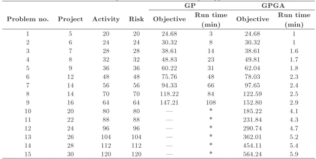
Table 9. Comparison between two developed approaches.
GP GPGA
Problem no. Project Activity Risk Objective Run time
(min) Objective
Run time (min)
1 5 20 20 24.68 3 24.68 1
2 6 24 24 30.32 8 30.32 1
3 7 28 28 38.61 14 38.61 1.6
4 8 32 32 48.83 23 49.81 1.7
5 9 36 36 60.22 31 62.04 1.8
6 12 48 48 75.76 48 78.03 2.3
7 14 56 56 94.33 66 97.65 2.4
8 14 70 70 118.22 84 122.59 2.5
9 16 64 64 147.21 108 152.80 2.9
10 20 80 80 | * 185.22 4.1
11 22 88 88 | * 231.84 4.3
12 24 96 96 | * 290.74 4.7
13 26 104 104 | * 362.01 5.2
14 28 112 112 | * 454.11 5.4
15 30 120 120 | * 564.24 5.9
Means the approach is not able to solve the instance in a reasonable run time.
the completion time. Benets grow by up to 5-time periods with the rate of 10%. The ratio of two objective functions is equal to 40 and their desired goals are determined by the application of two discrete uniform distributions of [0.2, 0.4, 0.6, 0.8, 1] and [30, 40, 50, 60, 70]. Duration of each activity is randomly specied based on an eight-digit discrete uniform distribution with numbers between [3, 10]. For assigning each risk to an activity of the project, risks and activities are randomly selected so that each activity is aected by only one risk. Also, the risk network of projects stating the interactions among risks is constructed as follows. First, among all projects, two projects are randomly selected and then, one risk is specied in each project. Finally, one of them is randomly selected to aect another one. This process continues as much as the number of projects. Also, by applying this process in each project, the interaction structure of risks is determined. Respective prior or conditional probabilities as well as the main time impact for each risk are specied by the application of continuous uniform distribution, i.e., [0 1]. Also, the intensifying impact of each risk is randomly determined according to the discrete uniform distribution with numbers [0.05, 0.1, 0.15, 0.2, 0.25].
6.2. Computational results
As mentioned earlier, ve small-size and ve medium-size instances have been designed to assess the e-ciency of the proposed GA approach compared with the exact solutions obtained by the GP method. The results for the generated instances are shown in Table 9. Table 9 indicates that the average error between the solutions of the two methods for the rst ten instances (small and medium sizes) is about 3%, which
shows that, on average, GA has generated near optimal solutions. On the other hand, the required run time of GA is signicantly less than that of the exact approach. Five large-size instances are designed and solved by this approach. As marked by (*), the exact approach is not able to solve the instances with sizes greater than 16 projects in a reasonable run time, i.e., less than two hours. Regarding the closeness of the solutions of the proposed GA to those of the exact approach, it has acceptable performance and is ecient and reliable enough to handle large-size instances and more realistic problems, which are not solvable using the exact method.
7. Conclusion
Project selection is a crucial decision in almost every company, particularly in project-based organizations, and has a signicant role in the performance of an or-ganization. Risks are the main causes of indeterminacy in projects and aect the duration of activities. This paper studied a novel formulation of the joint problem of project selection and scheduling by evaluating the individual and intensifying impacts of risks on duration of the activities of the projects. In the developed mathematical model, two objectives were considered. The rst objective was to minimize the aggregated risk and the second objective was to maximize the total benet of the projects, by which each project released a certain benet in each time period after its completion time. Regarding the risk network of the projects, stat-ing the potential risks and their interactions, Bayesian networks-based objective function was developed to evaluate the expected impacts of risks.
and scheduling projects in exact and approximate manners. The presented formulation provided a multi-objective mathematical model and the GP method was used to optimally select and schedule projects. Since the problem was NP-hard, an algorithm, which combined Goal Programming (GP) method and Ge-netic Algorithm (GA), named GPGA, was proposed. Then, the presented model was veried through a generated sample problem. Also, the eciency of the proposed metaheuristic algorithm compared with the exact approach was assessed through generating small- and medium-size instances. Accuracy of the generated solutions indicated that the metaheuristic algorithm had an acceptable eciency in dealing with large-size problems. To make the structure presented in this paper more applicable, it is suggested that this problem can be extended to resource-constraint project selection and scheduling or to a problem of selecting risk response strategies aimed at mitigating the impacts of risks.
References
1. Tuli, B., Arindam, S., Bijan, S., and Kumar, S.S. \Introduction to soft-set theoretic solution of project selection problem", Benchmarking: An International Journal, 23(7), pp. 1643-1657 (2016).
2. Rathi, R., Khanduja, D., and Sharma, S.K. \A fuzzy MADM approach for project selection: a six sigma case study", Decision Science Letters, 5(2), p. 14 (2016).
3. Tahri, H. \Mathematical optimization methods: ap-plication in project portfolio management", Procedia - Social and Behavioral Sciences, 210, pp. 339-347 (2015).
4. Namazian, A. and Haji Yakhchali, S. \Modeling and solving project portfolio and contractor selection prob-lem based on project scheduling under uncertainty", Procedia - Social and Behavioral Sciences, 226, pp. 35-42 (2016).
5. Badri, M.A., Davis, D., and Davis, D. \A comprehen-sive 0-1 goal programming model for project selection", International Journal of Project Management, 19(4), pp. 243-252 (2001).
6. Arratia M., N.M., Lopez I., F., Schaeer, S.E., and Cruz-Reyes, L. \Static R&D project portfolio selection in public organizations", Decision Support Systems, 84, pp. 53-63 (2016).
7. Tavana, M., Keramatpour, M., Santos-Arteaga, F.J., and Ghorbaniane, E. \A fuzzy hybrid project portfolio selection method using data envelopment analysis, TOPSIS and integer programming", Expert Systems with Applications, 42(22), pp. 8432-8444 (2015).
8. Fatemeh, P. and Sameh Monir, E.-S. \Project selection using the combined approach of AHP and LP", Journal of Financial Management of Property and Construc-tion, 21(1), pp. 39-53 (2016).
9. Kellenbrink, C. and Helber, S. \Scheduling resource-constrained projects with a exible project structure", European Journal of Operational Research, 246(2), pp. 379-391 (2015).
10. Ji, X. and Yao, K. \Uncertain project scheduling prob-lem with resource constraints", Journal of Intelligent Manufacturing, 28(3), pp. 575-580 (2017).
11. Toghian, A.A. and Naderi, B. \Modeling and solving the project selection and scheduling", Computers & Industrial Engineering, 83, pp. 30-38 (2015).
12. Doerner, K., Gutjahr, W.J., Hartl, R.F., Strauss, C., and Stummer, C. \Pareto ant colony optimization: A metaheuristic approach to multiobjective portfolio selection", Annals of Operations Research, 131(1), pp. 79-99 (2004).
13. Ghorbani, S. and Rabbani, M. \A new multi-objective algorithm for a project selection problem", Advances in Engineering Software, 40(1), pp. 9-14 (2009).
14. Medaglia, A.L., Graves, S.B., and Ringuest, J.L. \A multiobjective evolutionary approach for linearly constrained project selection under uncertainty", Eu-ropean Journal of Operational Research, 179(3), pp. 869-894 (2007).
15. Xiao, J., Ao, X.-T., and Tang, Y. \Solving software project scheduling problems with ant colony optimiza-tion", Computers & Operations Research, 40(1), pp. 33-46 (2013).
16. Wang, W.-X., Wang, X., Ge, X.-L., and Deng, L. \Multi-objective optimization model for multi-project scheduling on critical chain", Advances in Engineering Software, 68, pp. 33-39 (2014).
17. Perez, A., Quintanilla, S., Lino, P., and Valls, V. \A multi-objective approach for a project scheduling problem with due dates and temporal constraints infeasibilities", International Journal of Production Research, 52(13), pp. 3950-3965 (2014).
18. Minku, L.L., Sudholt, D., and Yao, X. \Improved evolutionary algorithm design for the project schedul-ing problem based on runtime analysis", IEEE Trans-actions on Software Engineering, 40(1), pp. 83-102 (2014).
19. Artigues, C., Leus, R., and Talla Nobibon, F. \Robust optimization for resource-constrained project schedul-ing with uncertain activity durations", Flexible Ser-vices and Manufacturing Journal, 25(1), pp. 175-205 (2013).
20. Suresh, M., Dutta, P., and Jain, K. \Resource con-strained multi-project scheduling problem with re-source transfer times", Asia-Pacic Journal of Opera-tional Research, 32(06), p. 1550048 (2015).
21. Aminbakhsh, S., Gunduz, M., and Sonmez, R. \Safety risk assessment using analytic hierarchy pro-cess (AHP) during planning and budgeting of construc-tion projects", Journal of Safety Research, 46, pp. 99-105 (2013).
22. Dikmen, I., Birgonul, M.T., and Han, S. \Using fuzzy risk assessment to rate cost overrun risk in interna-tional construction projects", Internainterna-tional Journal of Project Management, 25(5), pp. 494-505 (2007).
23. Shi-Ming, H., I-Chu, C., Shing-Han, L., and Ming-Tong, L. \Assessing risk in ERP projects: identify and prioritize the factors", Industrial Management & Data Systems, 104(8), pp. 681-688 (2004).
24. Kuo, Y.-C. and Lu, S.-T. \Using fuzzy multiple criteria decision making approach to enhance risk assessment for metropolitan construction projects", International Journal of Project Management, 31(4), pp. 602-614 (2013).
25. Rodrguez, A., Ortega, F., and Concepcion, R. \A method for the evaluation of risk in IT projects", Expert Systems with Applications, 45, pp. 273-285 (2016).
26. Zavadskas, E.K., Turskis, Z., and Tamosaitiene, J. \Risk assessment of construction projects", Journal of Civil Engineering and Management, 16(1), pp. 33-46 (2010).
27. Zeng, J., An, M., and Smith, N.J. \Application of a fuzzy based decision making methodology to construc-tion project risk assessment", Internaconstruc-tional Journal of Project Management, 25(6), pp. 589-600 (2007).
28. Cheng, M. and Lu, Y. \Developing a risk assess-ment method for complex pipe jacking construction projects", Automation in Construction, 58, pp. 48-59 (2015).
29. Jamshidi, A., Rahimi, S.A., Ait-kadi, D., Rebaiaia, M.L., and Ruiz, A. \Risk assessment in ERP projects using an integrated method", 3rd International Con-ference on Control, Engineering & Information Tech-nology (CEIT), Tlemcen, Algeria, pp. 1-5 (2015).
30. Ching-Chow, Y., Wen-Tsaan, L., Ming-Yi, L., and Jui-Tang, H. \A study on applying FMEA to improving ERP introduction: An example of semiconductor related industries in Taiwan", International Journal of Quality & Reliability Management, 23(3), pp. 298-322 (2006).
31. Gierczak, M. \The quantitative risk assessment of MINI, MIDI and MAXI horizontal directional drilling projects applying fuzzy fault tree analysis", Tunnelling and Underground Space Technology, 43, pp. 67-77 (2014).
32. Hyun, K.-C., Min, S., Choi, H., Park, J., and Lee, I.-M. \Risk analysis using fault-tree analysis (FTA) and analytic hierarchy process (AHP) applicable to shield TBM tunnels", Tunnelling and Underground Space Technology, 49, pp. 121-129 (2015).
33. Liang, W., Hu, J., Zhang, L., Guo, C., and Lin, W. \Assessing and classifying risk of pipeline third-party interference based on fault tree and SOM", Engineer-ing Applications of Articial Intelligence, 25(3), pp. 594-608 (2012).
34. Zeng, Y. and Skibniewski, M.J. \Risk assessment for enterprise resource planning (ERP) system implemen-tations: a fault tree analysis approach", Enterprise Information Systems, 7(3), pp. 332-353 (2013).
35. Pavlos, L. and Nick, F. \Risk and uncertainty in development: A critical evaluation of using the Monte Carlo simulation method as a decision tool in real estate development projects", Journal of Property Investment & Finance, 30(2), pp. 198-210 (2012).
36. Sadeghi, N., Fayek, A.R., and Pedrycz, W. \Fuzzy Monte Carlo simulation and risk assessment in con-struction", Computer-Aided Civil and Infrastructure Engineering, 25(4), pp. 238-252 (2010).
37. Chin, K.-S., Tang, D.-W., Yang, J.-B., Wong, S.Y., and Wang, H. \Assessing new product development project risk by Bayesian network with a systematic probability generation methodology", Expert Systems with Applications, 36(6), pp. 9879-9890 (2009).
38. Hu, Y., Zhang, X., Ngai, E.W.T., Cai, R., and Liu, M. \Software project risk analysis using Bayesian networks with causality constraints", Decision Support Systems, 56, pp. 439-449 (2013).
39. Luu, V.T., Kim, S.-Y., Tuan, N.V., and Ogun-lana, S.O. \Quantifying schedule risk in construction projects using Bayesian belief networks", International Journal of Project Management, 27(1), pp. 39-50 (2009).
40. Leu, S.-S. and Chang, C.-M. \Bayesian-network-based safety risk assessment for steel construction projects", Accident Analysis & Prevention, 54, pp. 122-133 (2013).
41. Sousa, R.L. and Einstein, H.H. \Risk analysis during tunnel construction using Bayesian networks: Porto Metro case study", Tunnelling and Underground Space Technology, 27(1), pp. 86-100 (2012).
42. Nordgard, D.E. and Sand, K. \Application of Bayesian networks for risk analysis of MV air insulated switch operation", Reliability Engineering & System Safety, 95(12), pp. 1358-1366 (2010).
43. Tang, C., Yi, Y., Yang, Z., and Sun, J. \Risk analysis of emergent water pollution accidents based on a Bayesian network", Journal of Environmental Management, 165, pp. 199-205 (2016).
44. Shabarchin, O. and Tesfamariam, S. \Internal cor-rosion hazard assessment of oil & gas pipelines us-ing Bayesian belief network model", Journal of Loss Prevention in the Process Industries, 40, pp. 479-495 (2016).
45. Khodakarami, V. and Abdi, A. \Project cost risk analysis: A Bayesian networks approach for model-ing dependencies between cost items", International Journal of Project Management, 32(7), pp. 1233-1245 (2014).
46. Tripathy, B.B. and Biswal, M.P. \A zero-one goal programming approach for project selection", Journal of Information and Optimization Sciences, 28(4), pp. 619-626 (2007).
Biographies
Ali Namazian received his BSc and MSc degrees in Industrial Engineering from Yazd University and Sharif University of Technology, Iran, respectively. He is currently a PhD candidate in Industrial Engineering at University of Tehran, Iran. His research interests include project selection and scheduling, project man-agement, multivariate and statistical analysis, multi-criteria decision-making, and advanced operation re-search.
Siamak Haji Yakhchali is an Assistant Professor of Industrial Engineering in the School of Industrial and Systems Engineering at the University of Tehran, Iran. He received his MSc and PhD degrees in Industrial
Engineering from Amirkabir University of Technology, Tehran, Iran. Also, he was a postdoctoral research fellow at the University College London. His expertise lies mainly in the eld of project scheduling and project management.
Masoud Rabbani is a Professor of Industrial En-gineering in the School of Industrial and Systems Engineering at the University of Tehran, Iran. He has published more than 50 papers in international jour-nals, e.g., European Journal of Operational Research, International Journal of Production Research, and International Journal of Production Economics. His current research interests comprise production plan-ning, applied graph theory, productivity management, and EFQM.