Sharif University of Technology
Scientia IranicaTransactions A: Civil Engineering http://scientiairanica.sharif.edu
Discharge and ow eld simulation of open-channel
sewer junction using articial intelligence methods
A.H. Zaji and H. Bonakdari
Department of Civil Engineering, Razi University, Kermanshah, Iran.
Received 13 December 2016; received in revised form 23 June 2017; accepted 29 August 2017
KEYWORDS Discharge prediction; Gene expression programming; Multiple non-linear regression;
Open channel; Radial basis neural network;
Sewer junction; Velocity eld.
Abstract. One of the most important parameters in designing sewer structures is the ability to accurately simulate their discharge and velocity eld. Among the various sewer receiving inow methods, open-channel junctions are the most frequently utilized ones. Because of the existence of separation and contraction zones in the open-channel junctions, the uid ow has a complex behavior. Modeling is carried out by Radial Basis Function (RBF) neural network, Gene Expression Programming (GEP), and Multiple Non-Linear Regression (MNLR) methods. Finding the optimum situation for GEP and RBF models is done by examining various mathematical and linking functions for GEP, dierent numbers of hidden neurons, and various spread amounts for RBF. In order to use the models in practical situations, three equations were conducted by using the RBF, GEP, and MNLR methods in modeling the longitudinal velocity. Then, the surface integral of the presented equations was used to simulate the ow discharge. The results showed that the GEP and RBF methods performed signicantly better than the MNLR in open-channel junction characteristics simulations. The GEP method had better performance than the RBF in modeling the longitudinal velocity eld. However, the RBF presented more reliable results in the discharge simulations.
© 2019 Sharif University of Technology. All rights reserved.
1. Introduction
Sewer junctions are widely used in the drainage struc-tures to collect the waste water. Fluid ows rarely ll the sewers under pressure. Instead, they often ow with air above the free surface and follow the open-channel hydraulic terms [1]. Junctions are one of the most typical inow receiver structures in sew-ers [2]. Due to the importance of modeling of the uid ow around junctions, the complex hydrodynamics of downstream ow have been studied in various re-searches, such as experimental studies [3-11], analytical
*. Corresponding author. Tel.: +98 831 427 4537; Fax: +98 831 428 3264
E-mail address: [email protected] (H. Bonakdari) doi: 10.24200/sci.2018.20695
investigations [12-14], and numerical modeling [15-22].
In the recent years, soft computing methods have widely been used in various engineering problems [23-27]. Complex ow velocity in the rivers was simulated by Kisi and Cigizoglu [28] using the RBF neural network. Bilhan et al. [29] simulated the side weir ow characteristics by using the RBF neural network. Azamathulla et al. [30] used GEP for modeling the accurate Manning roughness coecient. Zaji and Bonakdari [31] used the Multi-Layer Perceptron Ar-ticial Neural Network (MLP-ANN) and Genetic Pro-gramming (GP) in modeling the velocity eld around junctions. Bonakdari and Zaji [32] introduced a new Genetic Algorithm (GA) based Articial Neural Network (GA-ANN) method in order to simulate the open-channel junction velocity eld without needing to adjust the hidden layer neurons. The authors
con-cluded that GA-ANN method had better performance than other GA methods such as GP.
The aim of the present study is to obtain an analytical and, thus, continuous description of the complex discharge and velocity elds of open-channel sewer junction using the discrete laboratory measure-ments. To do that, some popular regression methods, namely, RBF, GEP, and MNLR, are developed. In the modeling procedure, the non-dimensional coordinate points (x, y, and z) and junction discharge ratio
(q) are considered as the input variable candidates
to predict the discharge and velocity elds. After nding the optimum input combination, three dierent equations are proposed to simulate the downstream longitudinal ow eld of the junction in the practical situations. Finally, the surface integral is used to reach the discharge simulation of the junction.
2. Experimental data
Weber et al. [11] performed a high quality experimental study on open-channel junctions, which has been uti-lized in various Computational Fluid Dynamic (CFD) studies in order to calibrate and validate the numerical models [16,17,20]. The result of the experimental mea-surements of Weber et al. [11] was used in this study in the training and testing processes of the investigated models. The experiments were performed in a junction ume with 0.91 m width and 90 conuence between
the main and tributary channels. The oor of the ume was horizontal and two head tanks were on the main and branch channels to supply the discharge. In order to have a completely developed ow near the junction, some perforated plates and honeycomb were placed at the beginning of the main and branch channels. The schematic overview of the laboratory ume is shown in Figure 1. The coordinates of each point were
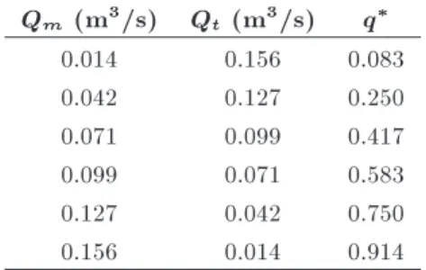
Table 1. The considered discharge ratios. Qm (m3/s) Qt (m3/s) q
0.014 0.156 0.083
0.042 0.127 0.250
0.071 0.099 0.417
0.099 0.071 0.583
0.127 0.042 0.750
0.156 0.014 0.914
non-dimensionalized by the channel width (x=b = x,
y=b = y, and z=b = z). The longitudinal velocity was
non-dimensionalized with the tail water velocity that remained constant in the experiments (u = u=0:628).
qin Eq. (1) is the ratio of the upstream to downstream
main channel discharges. q= Qm
Qm+ Qt; (1)
where Qm is the upstream main channel discharge
and Qt is the tributary discharge. This study was
conducted with various amounts of q, which are shown
in Table 1.
3. Methodology
In this section, the used numerical methods are investi-gated. Afterwards, the statistics that are used in order to evaluate performance of the model are represented. 3.1. Radial Basis Function (RBF) neural
network
Because of advantages such as easy design, high tolerance to input noise, good generalization of the nonlinear problems, and the ability of online learning, RBF has become one of the most popular neural network methods. The RBF [33,34] consists in some
radial functions. The amounts of the radial functions are directly related to the distance from the origin [35]. Input layer transforms the input variables into non-linear space by using the radial functions. After that, the output layer prepares the output of the model by using a linear regression between the radial functions. To this end, the output layer performs weighted sum-mation of the radial functions. Weight of each radial function indicates the impact of that function on the model output. These weights are determined by using the least squares method. The value of a radial basis, which is shown by '(x; c), increases with the radial distance r = kx ck, where x is the input and c is the radial function center. A radial function with N dimensions and the linear regression result of an RBF are shown in Eqs. (2) and (3), respectively.
f'(jjx xijj)ji = 1; 2; ; Ng; (2)
f(x) =
N
X
i=1
ci'(jjx xijj): (3)
With regards to the characteristic of linear determi-nation of the radial functions in the output layer, the RBF neural network is considered as one of the fast convergence neural networks [36].
Determination of the correct number of hidden layer neurons and the spread amount is one of the most important processes of the RBF modeling and directly aects the model performance. Trial and error method is applied in this study to the RBF code in order to determine the appropriate number of hidden neurons and spread amount [28,36].
3.2. Gene Expression Programming (GEP) The GEP, as a developed model of GP [37], is a computer program based method. The output of this method is presented by some subtrees that are linked with each other by linking mathematical functions. The algorithm of the GEP method is similar to that of the GA. However, GEP uses the computer programs instead of chromosomes in GA. First, the computer programs of the initial population are randomly gener-ated and, after that, the cost of each computer program is determined by using the considered tness function. Afterwards, by using the elite, mutation, and crossover processes, the next generation is constructed. GEP follows an evolutionary process and generation recon-struction is repeated until it reaches the determined number of generations or accuracy [38,39].
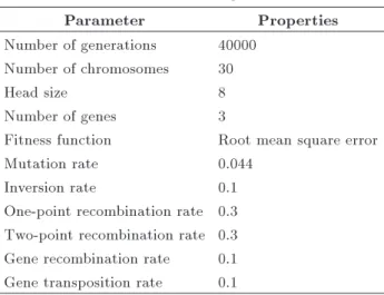
In this study, various functions, which are allowed to be used in the computer programs, and dierent subtree linking functions are investigated in order to nd the optimum GEP model. Other parameters of the models are presented in Table 2 according to Ferreira [39].
Table 2. GEP default parameters.
Parameter Properties
Number of generations 40000 Number of chromosomes 30
Head size 8
Number of genes 3
Fitness function Root mean square error
Mutation rate 0.044
Inversion rate 0.1
One-point recombination rate 0.3 Two-point recombination rate 0.3 Gene recombination rate 0.1 Gene transposition rate 0.1
3.3. Statistical errors
In order to have a comparison between the numerical models, the Mean Square Error (MSE), correlation coecient (R), Mean Absolute Error (MAE), average absolute deviation (%), Scatter Index (SI), and BIAS are used. The closer the amounts of the MSE, MAE, %, SI, and BIAS indices to zero and the closer the amount of R to one, the higher the performance of the models will be. The considered statistics are described in Eqs. (4)-(9).
MAE = 1 n Xn i=1 u
i;o ui;e; (4)
R =
n
P
i=1 u i;o uo
u
i;e ue
s n P i=1 u i;o uo
2 nP
i=1 u i;e ue
2; (5)
MSE = 1 n Xn i=1 u i;o ui;e
2 ; (6) % = n P i=1u
i;e ui;o n P i=1u i;e 100; (7) SI = s
(1=n)Pn
i=1
u
i;e ue ui;o uo 2
(1=n)Pn
i=1u i;o ; (8) BIAS = n P i=1 u
i;e ui;o
n : (9)
In this equations, u
i;o and ui;e are the ith
non-dimensional observed and estimated velocities, respec-tively, and n is the number of investigated samples.
4. Results and discussion
The aim of this section is to investigate the RBF, GEP, and MNLR methods in the open-channel junction longitudinal velocity eld and discharge simulations. Using the laboratory measurements of Weber et al. [11], a total of 5466 samples are used in order to develop the models. Also, 80% of the entire dataset (4373 samples) are separated randomly for the training process, and the remaining 20% (1093 samples) are considered as the testing dataset. The input variables of the models are non-dimensional coordinates of each point x, y,
and z as well as the discharge ratio q.
The results are presented in two parts. The goal of the rst part is to simulate the non-dimensional longitudinal velocity, u, by using the investigated
models. In addition, three dierent equations are proposed in this part that can simulate the velocity eld in the practical situations. In the second part, by using the surface integral equation, the downstream discharges of the junction are simulated and the results of the investigated models are compared.
4.1. Velocity eld simulation
The downstream longitudinal velocity eld of the open-channel junction is simulated in this section. The performance of the RBF is directly related to the optimum selection of the model's parameters. In order to nd the number of hidden layer neurons and the spread amount in the RBF neural network, two loops are added to the main RBF program, one for changing the spread amount and the other for changing the number of hidden layer neurons. Figure 2 shows the performance of each model with various spread amounts and hidden layer neuron numbers. In each situation, the performance of the model is represented by Root Mean Squared Error (RMSE). As it is shown in this gure, the RBF with 20 hidden layer neurons and the spread value of one has the most appropriate performance.
Figure 2. Spread and hidden neurons number determination of the RBF.
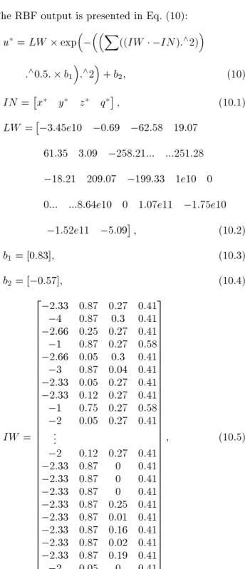
The RBF output is presented in Eq. (10): u= LW exp X((IW IN):^2)
:^0:5: b 1
:^2+ b
2; (10)
IN =x y z q; (10.1)
LW = 3:45e10 0:69 62:58 19:07 61:35 3:09 258:21::: :::251:28
18:21 209:07 199:33 1e10 0 0::: :::8:64e10 0 1:07e11 1:75e10
1:52e11 5:09; (10.2) b1= [0:83]; (10.3)
b2= [ 0:57]; (10.4)
IW = 2 6 6 6 6 6 6 6 6 6 6 6 6 6 6 6 6 6 6 6 6 6 6 6 6 6 6 6 6 6 6 6 6 6 6 6 6 6 4
2:33 0:87 0:27 0:41 4 0:87 0:3 0:41 2:66 0:25 0:27 0:41 1 0:87 0:27 0:58 2:66 0:05 0:3 0:41 3 0:87 0:04 0:41 2:33 0:05 0:27 0:41 2:33 0:12 0:27 0:41 1 0:75 0:27 0:58 2 0:05 0:27 0:41 ...
2 0:12 0:27 0:41 2:33 0:87 0 0:41 2:33 0:87 0 0:41 2:33 0:87 0 0:41 2:33 0:87 0:25 0:41 2:33 0:87 0:01 0:41 2:33 0:87 0:16 0:41 2:33 0:87 0:02 0:41 2:33 0:87 0:19 0:41 2 0:05 0 0:41 3 7 7 7 7 7 7 7 7 7 7 7 7 7 7 7 7 7 7 7 7 7 7 7 7 7 7 7 7 7 7 7 7 7 7 7 7 7 5 ; (10.5)
where IW and LW are the RBF coecients that are determined in the modeling process, b1 and b2 are
biases of the model, and IN is the input vector that contains the input variables of the model. It should be noted that in this equation, , +, and ^ are the
cell-by-cell operations.
Various parameters aect the GEP performance. Among them, the mathematical functions allowed to be used in the computer programs are the most important ones. Six dierent mathematical function combinations are examined in this study in order to nd the most
Table 3. Considered mathematical function combinations.
Function Denition RMSE
F 1 +, , , / 0.3399
F 2 +, , , /, p , Power 0.2456
F 3 +, , , /, p , Power, ln x, log x, ex, 10x 0.2620
F 4 +, , , /, p , Power, Average, Inverse 0.2778
F 5 +, , , /, p , p , Power, lnx, log x, e3 x, 10x, x2, x3, sin x, cos x, arctg x, negative, inverse 0.2534 F 6 +, , , /, p , ln x, ex, x2, arctg x, Inverse, tanh x, not, average, maximum, minimum 0.2464
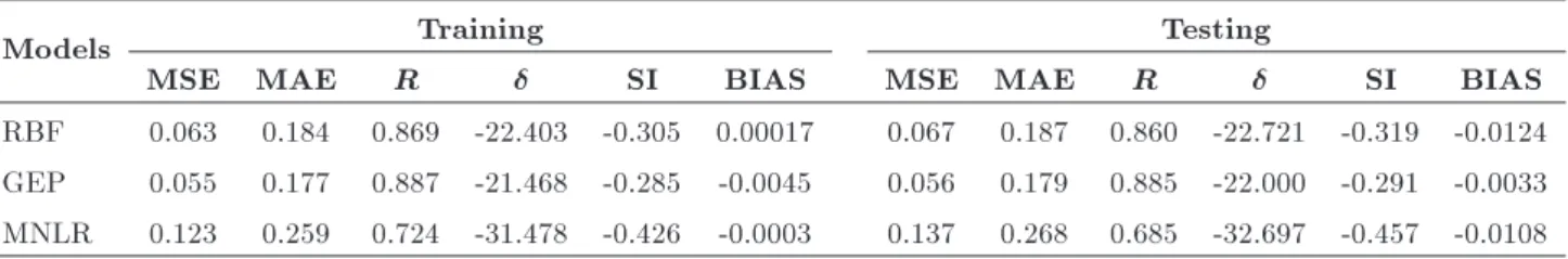
Table 4. Statistical indices for trained and tested datasets.
Models Training Testing
MSE MAE R SI BIAS MSE MAE R SI BIAS
RBF 0.063 0.184 0.869 -22.403 -0.305 0.00017 0.067 0.187 0.860 -22.721 -0.319 -0.0124 GEP 0.055 0.177 0.887 -21.468 -0.285 -0.0045 0.056 0.179 0.885 -22.000 -0.291 -0.0033 MNLR 0.123 0.259 0.724 -31.478 -0.426 -0.0003 0.137 0.268 0.685 -32.697 -0.457 -0.0108
appropriate one. According to Table 3, the F 2 mathematical function combination with the RMSE of 0.2456 has the best performance among the models. Moreover, it is obvious that increasing the complexity of the mathematical function combinations does not always lead to better performance of the computer programs.
As mentioned before, GEP's output is constructed from some subtrees. Subtrees are linked with each other by using a determined linking function. Many studies have used additional linking functions to con-nect the output subtrees [30,40-44]. However, in this study, the division linking function with RMSE of 0.2361 has the best performance in comparison with the addition, subtraction, and multiplication linking functions with RMSEs of 0.2456, 0.2820, and 0.2491, respectively. The output of the GEP model by using the second mathematical function combination and division linking function is presented in Eq. (11).
u=
2
4srq(q z)(qy) y
3 5
, z
xy2
yy,24 0:6730
q y
q
1:2522z y
3 5 :
(11) Another method investigated in this study is MNLR. The MNLR tries to nd a non-linear relationship between the considered input variables (x, y, z, and
q) and the output variable (u). The MNLR output
equation is presented in the following formula: u= (2:91)+( 0:02)x( 99:36)+( 4:27)y(0:11)
+(124:48) z(6:23)+( 104:31)q(33:76): (12)
Performances of the RBF, GEP, and MNLR models are shown in Table 4. According to this table, the GEP, with MSE of 0.056, has better performance than the RBF and MNLR models with MSEs of 0.067 and 0.137, respectively. In addition, it is evident that the GEP and RBF models are signicantly more accurate in simulating the open-channel junction longitudinal velocity eld simulation. The close performances of the considered models in test and train datasets show that there is no over-training occurring in the models. A comparison of the experimental measurements u with the RBF, GEP, and MNLR predictions for
u is presented in Figures 3, 4, and 5, respectively.
In each gure, the upper plot shows the comparison between the experimental and numerical u for the
entire test dataset and, in order to have a more detailed comparison, the lower plot compares the experimental
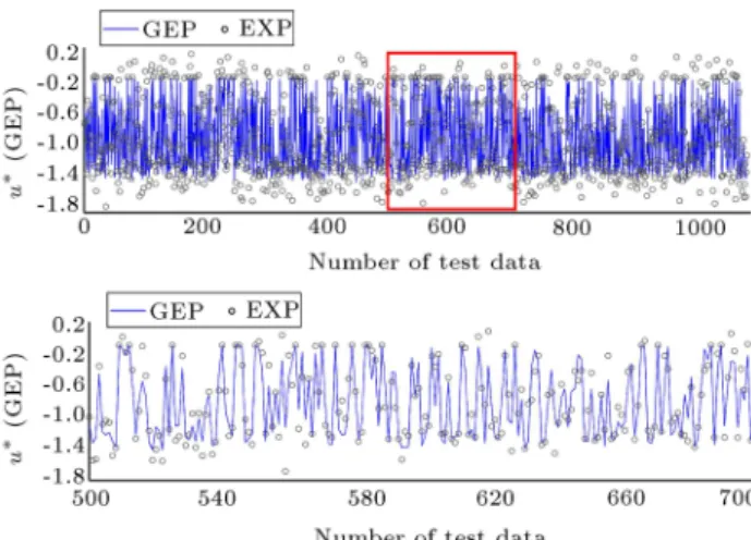
Figure 4. GEP modeling of u in test dataset.
Figure 5. MNLR modeling of uin test dataset.
and numerical u for the 500th to 700th samples of
the test dataset. From this gures, it can be seen that MNLR shows the worst performance in simulating the longitudinal velocity. The RBF and GEP models have close performances. However, according to the lower plots, it could be concluded that GEP has better performance in modeling the ow eld in the open-channel junctions.
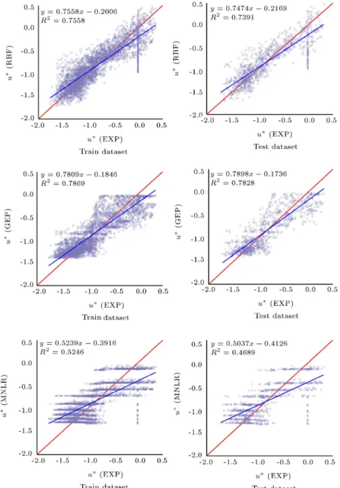
The scatter plots of the considered models for test and train datasets are presented in Figure 6. In this gure, the red line represents the exact 45 line. The
closer the scatters of a model to the exact line, the higher the accuracy of the model will be. The blue line in the plots shows the trend line of each dataset. The trend line has the equation of y = ax + b and closer a and b to one and zero, respectively, indicate the better performance of the models. From Figure 6, it is evident that the GEP model with a value of 0.7898, b value of 0.1736, and R2 value of 0.7828, in the test
dataset, has better performance than other models. The RBF model with a, b, and R2 of 0.7474, 0.2169,
and 0.7391, respectively, in test dataset, also has a good performance, which is highly close to the GEP model.
The MNLR is the weakest model that cannot simulate the complex velocity eld around the junctions to any degree.
4.2. Discharge simulation
Designing the sewer systems necessarily requires the ability to accurately predict the ow discharge. Be-cause of the crucial role of discharge in sewer structures, there are many studies performed on this topic [45-50]. Fortunately, using the u simulation developed in
the previous part and the surface integral on the cross section zones, the discharge of the junctions can be simulated. The discharge can be modeled by using u
according to the following equation: Q =x
A
udA; (13)
where Q is the discharge and u is the longitudinal
velocity of open-channel junction. In this equation, A represents the cross sections that are investigated in the x direction. In this study, the cross sections of
x = 1, -1.33, -1.66, -2, -2.33, -2.66, -3, -3.33, and
-3.66 are investigated according to Figure 1.
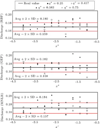
The results of the discharge simulation are plotted in Figure 7. In this gure, the discharges are simulated in various q amounts. In the experimental study
of Weber et al. [11], the junction outow discharge remains constant in all conditions up to 0.17 m3/s.
Therefore, the experimental results are plotted with a straight black line in the gure. It is obvious that the models with closer values of simulated discharge to this line have better performances. In order to investigate the performance of each model in discharge simulation, the Standard Deviation (SD) concept is used (Eq. (14)):
SD = v u u t 1
N 1
N
X
i=1
Resi
lineRes 2
; (14)
where Resi is the residual of the ith simulated sample
according to the experimental residual, Res is the average of the entire dataset residuals, and N is the number dataset's samples.
By denition, almost 95% of the dataset fre-quency is limited between Avg 2 SD and Avg + 2 SD. Avg is the average of the entire dataset. Ac-cording to Figure 7, despite the velocity eld prediction presented in the last part of results, the RBF model with Avg + 2 SD of 0.180 has better performance than the GEP model with Avg + 2 SD of 0.182. As an important result, the model with high accuracy in modeling of the ow eld velocity may have a worse performance in modeling of the discharge. In fact, high accuracy of the models in discharge prediction is dependent on their capability of simulating the mean
Figure 6. Experimental versus simulated u by RBF, GEP, and MNLR models.
velocity of the investigated section. As in the previous section, the MNLR model has worse performance than the RBF and GEP models.
5. Conclusion
Simulating the velocity eld and discharge of the sewer junctions was investigated in this study. In order to simulate the complex 3D downstream velocity eld of the junction, the non-dimensional coordinates of each point (x, y, and z) and discharge ratio (q) were
chosen as the input variables. The modeling processes were performed by using the RBF, GEP, and MNLR methods. In order to nd the optimum RBF model,
various numbers of hidden nodes and spread amounts were tested and the RBF with 20 hidden neurons and spread magnitude of one was chosen. The optimum GEP model was chosen by running the GEP with various linking and mathematical functions. Finally, the optimum GEP was found by using the combination of division linking function and +, , , =, p , and Power mathematical functions. Using the developed models, three dierent equations for modeling the longitudinal velocity in the open-channel junction were presented. The results of the velocity eld simulation showed that the GEP model performed better than the RBF and MNLR models. Afterwards, using the surface integral concept, discharge of the junction's
Figure 7. Discharge simulation with RBF, GEP, and MNLR models.
downstream ow was simulated. The results showed that despite the velocity prediction, the RBF method had higher accuracy in modeling the discharge than the GEP method. Therefore, it was concluded that a model with high accuracy in velocity eld prediction might be weak in discharge simulation. In both velocity eld and discharge simulations, the MNLR method performed signicantly worse than the RBF and GEP methods, and it was concluded that this model could not be used in the complex velocity prediction around the junction. Considering the practical equations presented in this study as well as the non-dimensional input and output variables used in the models, the results of the investigated methods can be utilized in the future researches and practical situations.
References
1. Yen, B.C. \Hydraulics of sewers", Adv. Hydrosci., 14, pp. 1-122 (1986).
2. Yekani Motlagh, Y., Nazemi, A.H., Sadraddini, A.A., Abbaspour, A., and Yekani Motlagh, S. \Numerical investigation of the eects of combining sewer junction characteristics on the hydraulic parameters of ow in fully surcharged condition", Water. Environ. J., 27(3), pp. 301-316 (2013).
3. Mosley, M.P. \An experimental study of channel con-uences", J. Geol., 84(5), pp. 535-562 (1976).
4. Ashmore, P. and Parker, G. \Conuence scour in coarse braided streams", Water. Resource. Res., 19(2), pp. 392-402 (1983).
5. Best, J.L. and Reid, I. \Separation zone at open-channel junctions", J. Hydraul. Eng., 110(11), pp. 1588-1594 (1984).
6. Biron, P., Roy, A., and Best, J. \Turbulent ow structure at concordant and discordant open-channel conuences", Exp. Fluids., 21(6), pp. 437-446 (1996).
7. Biron, P., Best, J.L., and Roy, A.G. \Eects of bed discordance on ow dynamics at open channel conuences", J. Hydraul. Eng., 122(12), pp. 676-682 (1996).
8. Kumar Gurram, S., Karki, K.S., and Hager, W.H. \Subcritical junction ow", J. Hydraul. Eng., 123(5), pp. 447-454 (1997).
9. Hsu, C.C., Wu, F.S., and Lee, W.J. \Flow at 90 equal-width open-channel junction", J. Hydraul. Eng., 124(2), pp. 186-191 (1998).
10. Ramamurthy, A.S. and Zhu, W. \Combining ows in 90 junctions of rectangular closed conduits", J. Hydraul. Eng., 123(11), pp. 1012-1019 (1997).
11. Weber, L.J., Schumate, E.D., and Mawer, N. \Exper-iments on ow at a 90 open-channel junction", J. Hydraul. Eng., 127(5), pp. 340-350 (2001).
12. Taylor, E.H. \Flow characteristics at rectangular open-channel junctions", T. Am. Soc. Civ. Eng., 109(1), pp. 893-902 (1944).
13. Modi, P.N., Ariel, P.D., and Dandekar, M.M. \Confor-mal mapping for channel junction ow", J. Hydraul. Div., 107(HY12, Proc. Paper 16763), pp. 1713-1733 (1981).
14. Hager, W.H. \Transitional ow in channel junctions", J. Hydraul. Eng., 115(2), pp. 243-259 (1989).
15. Bradbrook, K.F., Biron, P.M., Lane, S.N., Richards, K.S., and Roy, A.G. \Investigation of controls on secondary circulation in a simple conuence geometry using a three-dimensional numerical model", Hydrol. Proces., 12(8), pp. 1371-1396 (1998).
16. Huang, J., Weber, L.J., and Lai, Y.G. \Three-dimensional numerical study of ows in open-channel junctions", J. Hydraul. Eng., 128(3), pp. 268-280 (2002).
17. Shakibainia, A., Tabatabai, M.R.M., and Zarrati, A.R. \Three-dimensional numerical study of ow structure in channel conuences", Can. J. Civil. Eng., 37(5), pp. 772-781 (2010).
18. Bonakdari, H., Lipeme-Kouyi, G., and Wang, X. \Experimental validation of CFD modeling of multi-phase ow through open channel conuence", World Environmental and Water Resources Congress 2011: Bearing Knowledge for Sustainability, pp. 2176-2183 (2011).
19. Mignot, E., Bonakdari, H., Knothe, P., Lipeme Kouyi, G., Bessette, A., Rivire, N., and Bertrand-Krajewski, J. \Experiments and 3D simulations of ow structures
in junctions and their inuence on location of owme-ters", Water. Sci. Technol., 66(6), pp. 1325 (2012).
20. Yang, Q.Y., Liu, T.H., Lu, W.Z., and Wang, X.K. \Numerical simulation of conuence ow in open channel with dynamic meshes techniques", Adv. Mech. Eng., 5 (2013).
21. Sharipour, M., Bonakdari, H., Zaji, A.H., and Shamshirband, S. \Numerical investigation of ow eld and owmeter accuracy in open channel junctions", Eng. Appl. Comp. Fluid., 9(1), pp. 280-290 (2015).
22. Sharipour, M., Bonakdari, H., and Zaji, A. \Impact of the conuence angle on ow eld and owmeter accuracy in open channel junctions", International Journal of Engineering-Transactions B: Applications, 28(8), pp. 1145 (2015).
23. Najafzadeh, M. and Bonakdari, H. \Application of a neuro-fuzzy GMDH model for predicting the ve-locity at limit of deposition in storm sewers", Jour-nal of Pipeline Systems Engineering and Practice, p. 06016003 (2016).
24. Najafzadeh, M., Balf, M.R., and Rashedi, E. \Pre-diction of maximum scour depth around piers with debris accumulation using EPR, MT, and GEP mod-els", Journal of Hydroinformatics, 18(5), pp. 867-884 (2016).
25. Kaydani, H., Najafzadeh, M., and Mohebbi, A. \Well-head choke performance in oil well pipeline systems based on genetic programming", Journal of Pipeline Systems Engineering and Practice, 5(3), p. 06014001 (2014).
26. Najafzadeh, M., Laucelli, D.B., and Zahiri, A. \Ap-plication of model tree and evolutionary polynomial regression for evaluation of sediment transport in pipes", KSCE Journal of Civil Engineering, 21(5), pp. 1956-1963 (2016).
27. Najafzadeh, M., Tafarojnoruz, A., and Lim, S.Y. \Pre-diction of local scour depth downstream of sluice gates using data-driven models", ISH Journal of Hydraulic Engineering, 23(2), pp. 195-202 (2017).
28. Kisi, O. and Cigizoglu, H.K. \Comparison of dierent ANN techniques in river ow prediction", Civ. Eng. Environ. Syst., 24(3), pp. 211-231 (2007).
29. Bilhan, O., Emin Emiroglu, M., and Kisi, O. \Appli-cation of two dierent neural network techniques to lateral outow over rectangular side weirs located on a straight channel", Adv. Eng. Software., 41(6), pp. 831-837 (2010).
30. Azamathulla, H.M., Ahmad, Z., and Ab. Ghani, A. \An expert system for predicting Manning's roughness coecient in open channels by using gene expression programming", Neural. Comput. Appl., 23(5), pp. 1343-1349 (2013).
31. Zaji, A.H. and Bonakdari, H. \Application of articial neural network and genetic programming models for estimating the longitudinal velocity eld in open chan-nel junctions", Flow. Meas. Instrum., 41, pp. 81-89 (2015).
32. Bonakdari, H. and Zaji, A.H. \Open channel junction velocity prediction by using a hybrid self-neuron ad-justable articial neural network", Flow Measurement and Instrumentation, 49, pp. 46-51 (2016).
33. Broomhead, D.S. and Lowe, D. \Radial basis func-tions, multi-variable functional interpolation and adaptive networks", Royal. Signals. Radar. Est. Memo., 4248 (1988).
34. Poggio, T. and Girosi, F. \Regularization algorithms for learning that are equivalent to multilayer net-works", Science, 247(4945), pp. 978-982 (1990).
35. Buhmann, M.D., Radial Basis Functions: Theory and Implementations, Cambridge University Press Cam-bridge (2003).
36. Kisi, O. \The potential of dierent ANN techniques in evapotranspiration modelling", Hydrol. Proces., 22(14), pp. 2449-2460 (2008).
37. Koza, J.R. \Genetic programming as a means for programming computers by natural selection", Stat. Comput., 4(2), pp. 87-112 (1994).
38. Ferreira, C. \Gene expression programming in prob-lem solving", In Soft. Comput. Indust., pp. 635-653, Springer (2002).
39. Ferreira, C. \Gene expression programming: A new adaptive algorithm for solving problems", Complex. Sys., 13(2), pp. 87-129 (2001).
40. Aytek, A. and Kisi, O. \A genetic programming ap-proach to suspended sediment modelling", J. Hydrol., 351(3-4), pp. 288-298 (2008).
41. Ab Ghani, A. and Md Azamathulla, H.
\Gene-expression programming for sediment transport in sewer pipe systems", J. Pipeline. Syst. Eng. Pract., 2(3), pp. 102-106 (2011).
42. Shiri, J. and Kisi, O. \Comparison of genetic pro-gramming with neuro-fuzzy systems for predicting short-term water table depth uctuations", Comput. Geosci., 37(10), pp. 1692-1701 (2011).
43. Onen, F. \GEP prediction of scour around a side weir in curved channel", J. Environ. Eng. Landsc. Manage., 22(3), pp. 161-170 (2014).
44. Kisi, O., Dailr, A.H., Cimen, M., and Shiri, J. \Sus-pended sediment modeling using genetic programming and soft computing techniques", J. Hydrol., 450-451, pp. 48-58 (2012).
45. Isel, S., Dufresne, M., Bardiaux, J.B., Fischer, M., and Vazquez, J. \Computational uid dynamics based assessment of discharge-water depth relationships for combined sewer overows", Urban. Water. J., 11(8), pp. 631-640 (2014).
46. Regneri, M., Klepiszewski, K., Seiert, S., Vanrol-leghem, P.A., and Ostrowski, M. \Transport sewer model calibration by experimental generation of dis-crete discharges from individual CSO structures", iEMSs 2012 - Managing Resources of a Limited Planet: Proceedings of the 6th Biennial Meeting of the Interna-tional Environmental Modelling and Software Society, pp. 3109-3116 (2012).
47. Bonakdari, H. \Simple method for the estimation of discharge by entropy in narrow compound sewers", Can. J. Civil. Eng., 39(3), pp. 339-343 (2012).
48. Fach, S., Sitzenfrei, R., and Rauch, W. \Determining the spill ow discharge of combined sewer overows using rating curves based on computational uid dy-namics instead of the standard weir equation", Water Sci. Technol., 60(12), pp. 3035-3043 (2009).
49. Oliveto, G. and Hager, W.H. \Discharge measurement in circular sewer", J. Irrig. Drain. Eng., 123(2), pp. 138-140 (1997).
50. Payne, J.A. and Hedges, P.D. \An evaluation of the impacts of discharges from surface water sewer outfalls", Water. Sci. Technol., 22(10-11), pp. 127-135 (1990).
Biographies
Amir Hossein Zaji is now PhD student in Civil Engineering with specialty in Hydraulic Structures in the Department of Civil Engineering, Razi University, Kermanshah, Iran. He has more than 30 published papers in ISI journals. He works in eld of soft computing methods in engineering applications. Hossein Bonakdari is Professor in the Department
of Civil Engineering at Razi University. He received his PhD in Civil Engineering from University of Caen, France. After obtaining PhD, he joined Razi University as a faculty member in 2006 and, presently, he is a Full Professor in the Department of Civil Engineering. He has supervised 5 PhD and 30 MS theses with teaching experience of more than 16 years in the eld of civil engineering. From 2010 to 2011, he was researcher at Laboratory of Civil and Environmental Engineering, INSA of Lyon, France; from 2011 to 2013, Deputy of Planning & Development in National Water and Wastewater Engineering Company, Iran; and from 2013 to 2015, Director General of Training, Research and Technology Development at Ministry of Energy, Iran. His elds of specialization and interest include practical application of soft computing in engineer-ing, modeling of wastewater urban drainage systems, sediment transport, computational uid dynamics and hydraulics, design of hydraulic structures, and uid mechanics. The results of his researches have been published in more than 130 papers in international journals (h-index = 13). He has also more than 150 presentations in national and international conferences and 2 books. He has been rated as distinguished researcher at Razi University in 2014, 2015, and 2016.