A multi-period fuzzy mathematical programming model for crude oil supply
chain network design considering budget and equipment limitations
Armin Jabbarzadeh
1*, Mir Saman Pishvaee
1, Ali Papi
11 School of Industrial Engineering, Iran University of Science and Technology, Tehran, Iran
[email protected], [email protected], [email protected]
Abstract
The major oil industry upstream activities include the exploration, drilling, extraction, pipelines installation, and production of crude oil. In this paper, we develop a mathematical model to plan for these operations as a crude oil supply chain network design problem. The proposed multi-period mixed integer linear programming model entails both strategic (e.g., facility location and allocation) and tactical (e.g., project and production planning) decisions. With the objective of maximizing total Net Present Value (NPV) at the end of planning horizon, the decisions to be made comprise the location of the facilities, the flow of commodities and the amount of investment. The uncertain natures of important input parameters such as capital and operational cost, demand and price of crude oil, are taken into account via fuzzy theory. Finally, the performance of the developed model is investigated using the real data of Iranian South Oilfields.
Keyword:
Crude oil supply chain, oilfield development, multi-period programming, time horizon analysis, fuzzy optimization.1- Introduction
Supply chain management (SCM) is the management of the flow of goods and services. It includes the movement and storage of raw materials, inventory, and finished goods from point of origin to point of consumption. Applying the concept of supply chain management can provide considerable competitive advantage for any companies from any sectors (Damghani, 2015). In this context, the petroleum/oil industry can be characterized as a supply chain which is of vital importance in the economy of the world oil-rich countries. The optimization of such a supply chain can significantly increase the profitability of oil companies and improve the national economic indices.
A typical oil industry supply chain is composed of an exploration operation at well heads,
crude procurement and storage logistics, transportation to refineries, refinery operations, and
distribution of products. These activities can be classified into two categories.
*Corresponding author.
ISSN: 1735-8272, Copyright c 2016 JISE. All rights reserved
Journal of Industrial and Systems Engineering
Vol. 9, special issue on supply chain, pp 88 – 107
Winter (January) 2016
The first category includes upstream activities such as exploration, well drilling, crude oil
extraction and crude oil production. These operations are related to the crude oil supply chain.
The second section includes downstream (Refinery) operations such as (I) crude-oil unloading,
mixing and inventory control, (II) scheduling of production units, and (III) finish products
blending and distribution. The problems related to the second category can be formulated as
downstream oil supply chain problems. Also, all the activities can be considered as petroleum
supply chain problems.
Upstream activities such as investment planning, facility location- allocation, and production planning, which also called oilfields development, can be modeled as crude oil supply chain (Sahebi et al., 2014) or upstream petroleum supply chain. Shah et al. (2011) explained crude oil supply chain based on the strategic and tactical levels of decision making as follows:
Facility location and allocation: selection of optimal locations for drilling, installation of platforms and production units (PU), and allocation of facilities (Strategic level).
Project planning: determination of the optimal time for drilling, installation of the equipment, and construction of facilities required for production (Tactical level).
Production planning: determination of the optimal extraction of each well considering the reservoir behavior, and the amount of optimal production (Tactical and operational levels).
One of the earliest works in the oilfield development is contributed by Devine and Lesso (1972). They address to location and allocation of the well, and facility related to oilfield. Iyer et al. (1998) proposed a multi-period MILP model for optimal project planning as well as facility location and allocation of offshore oilfield development. They approximated reservoirs performance equations through piecewise linear approximations. This work was extended by van den Heever and Grossmann (2000) where they proposed a multi-period generalized disjunctive programming model for oil field infrastructure planning and a bi-level decomposition method to solve the developed model. Kosmidis et al. (2002) considered a mixed integer optimization strategy for integrated oil and gas production. They presented a dynamic optimization model and an efficient approximation solution strategy for this system. Kosmidis et al. (2004) also proposed a mixed integer nonlinear (MINLP) model for the daily well scheduling in oilfields, where nonlinearity behavior for reservoirs was considered. Carvalho and Pinto (2006a) extended the model developed by (Tsarbopoulou, 2000), and proposed a bi-level decomposition algorithm for solving large scale problems where the master problem determines the allocation of platforms to wells and sub-problem is related to scheduling of the fixed facilities. This model was further extended by (Carvalho and Pinto, 2006b) where multiple reservoirs were considered within the model.
All the above-mentioned papers applied deterministic mathematical programming approaches; however, the assumption of certainty for some parameters of problem such as demand, oil price, costs, etc., and other important ones like productivity index, reservoirs behavior may lead to inefficient results. Aseeri et al. (2004) considered uncertainty in some parameters such as the oil prices and well productivity index (PI) into the model proposed by (Iyer et al., 1998) and used the approximation algorithm to solve the corresponding stochastic programming model. Tarhan et al. (2009) presented a multistage stochastic programming model for planning offshore oilfields infrastructure in stochastic environment. They considered uncertainty in initial maximum oil flow rate and recoverable oil volume.
In the recent papers of this context, Gupta and Grossmann (2012) proposed a novel mathematical model for optimal planning of offshore oil and gas field infrastructure. Then, this model was developed by a multistage stochastic programming to regard uncertainty of parameters (Gupta and Grossmann,
2014). Also, about the maritime transportation of crude oil, Hennig et al. (2012) applied a mathematical programming model to describe the distribution of crude oil from supply places to demand point. Shen et al. (2011) introduced a Lagrangian relaxation approach for an inventory-routing problem with transshipment in crude oil transportation.
In this paper, we present a multi-period mathematical programming model which takes all of the strategic, tactical and operational activity into account in a fuzzy environment integrally. According to this model, offshore oilfield development operations (e.g. drilling, extraction, pipelines installation, and production of crude oil) are expressed as a mixed integer linear programming (MILP) problem. Furthermore, the lack of consideration of budget, time, and equipment limitations constraints which may far previous study away from real world, is intended in this work. In other word, the aim of this paper is development of optimization model for upstream oil industry activities as crude oil supply chain, in which net present value (NPV) of crude oil sale is maximized, while all of the constraints about oilfield development such as extract-rig limitation, production capacity, transport-rig limitation as well as budget and investment limitation should be satisfied.
The rest of paper is organized as follows: Next section gives an explanation of problem and describes the crude oil supply chain structure precisely. The proposed fuzzy mathematical programming model is elaborated in the ‘Modeling’ Section. ‘Model performance, result and discussion’ section reports the numerical results, sensitivity analysis, validation of approach and a managerial discussion of the results. Finally, ‘Conclusion’ section concludes the paper as well as introducing a number of attractive future research directions.
2- Problem definition
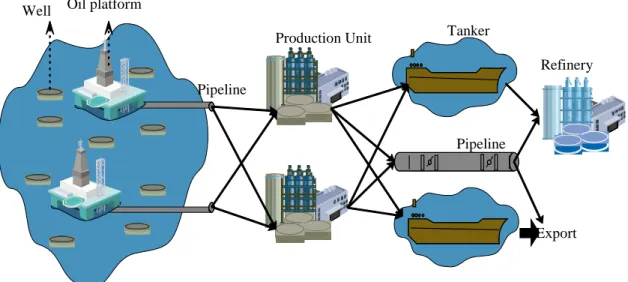
Consider an oilfield which consists of a set of explored oil reservoirs and wells. To appropriately exploit oilfield reservoirs, it is necessary to provide the capital and equipment required for drilling, extraction, production, supply and transfer. The first step, after exploration of reservoirs and oilfields, is drilling wells and then extraction for which well platforms are installed. The extracted crude oil which is usually mixed with water is transferred through pipelines to the production unit (PU) where impurities are separated and then the crude oil is ready to be supplied to customers (local refineries and exportation) (see Figure1).
The crude oil is transferred to local customers mostly through pipelines. Although the same is possible for exportation, it is usually carried out through marine terminals from where the oil is transferred overseas by big tankers. The transportation part of this problem is the crude oil transfer from well to PUs as well as from PUs to local refineries and exportation terminals through pipelines.
Depending on the oil reservoirs behavior and the available equipment, exploitation usually takes about fifteen to twenty years (Gupta and Grossmann, 2012, Sahebi and Nickel, 2014). During the planning horizon, the revenue from crude oil selling, the costs rigs and facilities as well as operational cost should be considered simultaneously to make optimal decisions.
Figure 1.The network of crude oil supply chain
In order to provide a better description from the concerned problem, consider a proved oilfield consisting of several reservoirs where each of them contains a number of potential wells with specific productivity index (PI) and oil-water ratio (OWR) as well as some offshore platforms types and production rigs to recover oil from the wells and preparing it to supply. A set of pipes are available to pump crude oil from wells to PUs, and from PUs to customers, who have demand for produced crude oil. The optimal decision making about operations, transportation, and investment planning is main problem that divided to some sub-problems as follows:
I. Which wells and in which periods should be drilled?
• The answer of this problem is obtained by PI and OWR indices of wells. II. Which well/oil platforms (WPs) should be installed for drilling and extraction?
• The answer of this problem is obtained by the capital and operational cost, and capacity of WPs.
III. What type of pipes should be installed in different transportation lines?
• The answer of this problem is obtained by the capital cost of pipes and their capacity. IV. Where PUs should be located?
• The answer of this problem is obtained according to distances between wells to PUs, and PUs to customers.
V. How much crude oil should/may be extracted in each period, and how much is production
volume?
• The answer of this problem is obtained according to PI and OWR indices of drilled wells, capacity of available PUs, and amount of customers demand.
VI. How much capital should be invested in each period?
• The answer of this problem is obtained according to facility and budget limitations.
Tanker
Pipeline
Export Refinery Production Unit
Well Oil platform
Pipeline
In the concerned problem, an oil company (company that produce and supply crude oil) aims to make decisions optimally about above sub-problems. As mentioned above, the objective of this company is to maximize the NPV of crude oil sale. It is obvious that in order to achieve this objective, the company managers solve an optimization problem consisting facility selection (I, II, III), facility location and allocation (IV), production planning (V), and investment planning (VI).
Some parameters such as the capital and operational costs of facilities (WPs, PUs), transportation cost, wells indices (PI, OWR), and finally oil price and demand are to be specified during each period throughout the planning time horizon. Although estimation of the values of some of these parameters is possible based on the existing data and experts’ opinions, they are undoubtedly imprecise and associated with uncertainties; therefore, in this research, these values have been considered as triangular fuzzy numbers to somewhat take into account the uncertainties governing the system. Thus, a fuzzy optimization problem is developed, which the solution of it can be useful for managers decision making.
3- Model formulation
3-1- Problem representation as a mathematical programming
In the following a mixed integer linear programming formulation is presented for the in hand problem. The nomenclature used in our model is as follows:
Index Description
𝑤𝑤 potential well, 𝑤𝑤 ∈ 𝑊𝑊 = {1, 2, … , |𝑊𝑊|}
𝑤𝑤𝑝𝑝 potential well platform, 𝑤𝑤𝑝𝑝 ∈ 𝑊𝑊𝑃𝑃 = {1, 2, … , |𝑊𝑊𝑃𝑃|}
𝑝𝑝𝑢𝑢 location of Production Unit, 𝑝𝑝𝑢𝑢 ∈ 𝑃𝑃𝑈𝑈 = {1, 2, … , |𝑃𝑃𝑈𝑈|} 𝑝𝑝𝑙𝑙 pipeline types, 𝑝𝑝𝑙𝑙 ∈ 𝑃𝑃𝐿𝐿 = {1, 2, … , |𝑃𝑃𝐿𝐿|}
𝑐𝑐𝑑𝑑 domestic customer, 𝑐𝑐𝑑𝑑∈ 𝐶𝐶𝑑𝑑= {1, 2, … , |𝐶𝐶𝑑𝑑|}
𝑐𝑐𝑓𝑓 foreign customer, 𝑐𝑐𝑓𝑓 ∈ 𝐶𝐶𝑓𝑓 = �1, 2, … , �𝐶𝐶𝑓𝑓�� 𝑐𝑐 customer, 𝑐𝑐 ∈ 𝐶𝐶 = �1, 2, … , |𝐶𝐶𝑑𝑑| + |𝐶𝐶𝑓𝑓|�
𝑡𝑡 Time horizon, 𝑡𝑡 ∈ 𝑇𝑇 = {1, 2, … , |𝑇𝑇||}
Deterministic
parameters Description
𝑈𝑈 𝑡𝑡𝑤𝑤𝑝𝑝 maximum extraction capacity of the 𝑤𝑤𝑝𝑝th well platform in period 𝑡𝑡 𝑈𝑈𝑡𝑡𝑝𝑝𝑢𝑢 maximum production capacity of the 𝑝𝑝𝑢𝑢th production unit in period 𝑡𝑡 𝑈𝑈𝑡𝑡𝑝𝑝𝑙𝑙 maximum transportation capacity of the 𝑝𝑝𝑙𝑙th pipeline in period 𝑡𝑡
𝐿𝐿𝑛𝑛𝑛𝑛(𝑤𝑤𝑝𝑝 ,𝑝𝑝𝑢𝑢) distance between 𝑤𝑤𝑝𝑝th well platform (or well) and 𝑝𝑝𝑢𝑢th production unit
𝐿𝐿𝑛𝑛𝑛𝑛(𝑝𝑝𝑢𝑢 ,𝑐𝑐) distance between 𝑝𝑝𝑝𝑝th production unit and 𝑐𝑐th customer
Uncertain parameters
Description
𝑃𝑃𝐼𝐼𝑡𝑡𝑤𝑤 Productivity Index of 𝑤𝑤th well in period 𝑡𝑡
𝑝𝑝𝑑𝑑𝑡𝑡𝑤𝑤 maximum Pressure Drop from 𝑤𝑤th well bore to well head in period 𝑡𝑡
𝑂𝑂𝑊𝑊𝑊𝑊𝑡𝑡𝑤𝑤 maximum oil-to-water flow rate of the 𝑤𝑤th well in period 𝑡𝑡
𝐼𝐼𝑛𝑛𝑛𝑛𝑡𝑡𝑊𝑊 maximum budget which can be invested in well drilling in period 𝑡𝑡
𝐼𝐼𝑛𝑛𝑛𝑛𝑡𝑡𝑊𝑊𝑃𝑃 maximum budget which can be invested in well platform installing in period 𝑡𝑡
𝐼𝐼𝑛𝑛𝑛𝑛𝑡𝑡𝑃𝑃𝑈𝑈 maximum budget which can be invested in production unit constructing in period
𝑡𝑡
𝐿𝐿𝑡𝑡 maximum length of pipeline which can be installed during period 𝑡𝑡
𝑈𝑈𝑁𝑁𝑡𝑡𝑊𝑊 maximum number of the well which can be drilled in period 𝑡𝑡
(Because of time and equipment limitation)
𝑈𝑈𝑁𝑁𝑡𝑡𝑊𝑊𝑃𝑃 maximum number of the well platform which can be installed in period 𝑡𝑡
𝑈𝑈𝑁𝑁𝑡𝑡𝑃𝑃𝑈𝑈 maximum number of the production unit which can be constructed in period
𝐷𝐷𝑡𝑡𝑐𝑐 demand volume of the 𝑐𝑐th customer in period 𝑡𝑡
𝛼𝛼𝑡𝑡𝑐𝑐𝑓𝑓 minimum percent of oil supply to 𝑐𝑐
𝑓𝑓th foreign customer in period 𝑡𝑡
𝛽𝛽𝑡𝑡𝑐𝑐𝑑𝑑 minimum percent of oil supply to 𝑐𝑐
𝑑𝑑th domestic customer in period 𝑡𝑡
𝑑𝑑𝑡𝑡 price deflator index in period 𝑡𝑡
𝑃𝑃𝑡𝑡𝑐𝑐 sale price of oil for 𝑐𝑐th customer in period 𝑡𝑡
𝐵𝐵𝑡𝑡∗ Drilling (∗ = 𝑤𝑤) or installing (∗ = 𝑤𝑤𝑝𝑝 𝑜𝑜𝑟𝑟 𝑝𝑝𝑢𝑢 𝑜𝑜𝑟𝑟 𝑝𝑝𝑙𝑙) cost of the 𝑓𝑓th facility in
period 𝑡𝑡
𝐹𝐹𝐶𝐶𝑡𝑡𝑤𝑤𝑝𝑝 fixed operation cost of 𝑤𝑤𝑝𝑝th well platform in period 𝑡𝑡 𝐹𝐹𝐶𝐶𝑡𝑡𝑝𝑝𝑢𝑢 fixed operation cost of 𝑝𝑝𝑢𝑢th production unit in period 𝑡𝑡
𝐸𝐸𝑥𝑥𝑡𝑡𝑤𝑤𝑝𝑝 extraction cost per unit of fluid extracted by the 𝑤𝑤𝑝𝑝th well platform in period 𝑡𝑡 fixed operation cost of facility 𝑓𝑓 in period 𝑡𝑡
𝑃𝑃𝑟𝑟𝐶𝐶𝑡𝑡𝑝𝑝𝑢𝑢 production cost per unit of crude oil produced by the 𝑝𝑝𝑢𝑢th production unit in period
𝑡𝑡
Integer
variables Description
𝑌𝑌𝑡𝑡∗ 1 if the 𝑓𝑓th well (∗ = 𝑤𝑤) is drilled, well platform (∗ = 𝑤𝑤𝑝𝑝) is installed,
production unit (∗ = 𝑝𝑝𝑢𝑢) is built in period𝑡𝑡; else 0.
𝑌𝑌𝑡𝑡(𝑤𝑤,𝑤𝑤𝑝𝑝) 1 if the interconnection between w and 𝑤𝑤𝑝𝑝 is installed in period 𝑡𝑡; else 0. 93
𝑌𝑌𝑡𝑡𝑝𝑝𝑙𝑙,(𝑤𝑤𝑝𝑝,𝑝𝑝𝑢𝑢) 1 if the 𝑝𝑝𝑙𝑙th type of pipes is installed in period 𝑡𝑡 between 𝑤𝑤𝑝𝑝 and 𝑝𝑝𝑝𝑝; else 0. 𝑌𝑌𝑡𝑡𝑝𝑝𝑙𝑙,(𝑝𝑝𝑢𝑢,𝑐𝑐) 1 if the 𝑝𝑝𝑙𝑙th type of pipes is installed in period 𝑡𝑡 between 𝑝𝑝𝑢𝑢 and 𝑐𝑐; else 0.
𝑜𝑜𝑝𝑝𝑝𝑝𝑛𝑛𝑡𝑡∗ 1 if the 𝑓𝑓th well (∗ = 𝑤𝑤) is open, well platform (∗ = 𝑤𝑤𝑝𝑝) is open, production unit
(∗ = 𝑝𝑝𝑢𝑢) is open in period𝑡𝑡; else 0.
𝑜𝑜𝑝𝑝𝑝𝑝𝑛𝑛𝑡𝑡(𝑤𝑤,𝑤𝑤𝑝𝑝) 1 if the interconnection between w and 𝑤𝑤𝑝𝑝 is open in period 𝑡𝑡; else 0. 𝑜𝑜𝑝𝑝𝑝𝑝𝑛𝑛𝑡𝑡𝑝𝑝𝑙𝑙,(𝑤𝑤𝑝𝑝,𝑝𝑝𝑢𝑢) 1 if the 𝑝𝑝𝑙𝑙th type of pipes is open in period 𝑡𝑡 between 𝑤𝑤𝑝𝑝 and 𝑝𝑝𝑝𝑝; else 0. 𝑜𝑜𝑝𝑝𝑝𝑝𝑛𝑛𝑡𝑡𝑝𝑝𝑙𝑙,(𝑝𝑝𝑢𝑢,𝑐𝑐) 1 if the 𝑝𝑝𝑙𝑙th type of pipes is open in period 𝑡𝑡 between 𝑝𝑝𝑢𝑢 and 𝑐𝑐; else 0.
Continuous
variables Description
𝑜𝑜𝑖𝑖𝑙𝑙𝑡𝑡𝑤𝑤,𝑤𝑤𝑝𝑝 extracted oil volume from the 𝑤𝑤th well by the 𝑤𝑤𝑝𝑝th well platform in period 𝑡𝑡
𝑤𝑤𝑎𝑎𝑡𝑡𝑝𝑝𝑟𝑟𝑡𝑡𝑤𝑤,𝑤𝑤𝑝𝑝 extracted water volume from the 𝑤𝑤th well by the 𝑤𝑤𝑝𝑝th well platform in period 𝑡𝑡
period 𝑡𝑡
𝑜𝑜𝑖𝑖𝑙𝑙𝑡𝑡𝑤𝑤𝑝𝑝,𝑝𝑝𝑢𝑢 transported oil volume from the 𝑤𝑤𝑝𝑝th well platform to the 𝑝𝑝𝑢𝑢th production unit in
period 𝑡𝑡
𝑤𝑤𝑎𝑎𝑡𝑡𝑝𝑝𝑟𝑟𝑡𝑡𝑤𝑤𝑝𝑝,𝑝𝑝𝑢𝑢 transported water volume from the 𝑤𝑤𝑝𝑝th well platform to the 𝑝𝑝𝑢𝑢th production unit
in period𝑡𝑡
𝑓𝑓𝑙𝑙𝑑𝑑𝑡𝑡𝑤𝑤𝑝𝑝 total extracted fluids at the 𝑤𝑤𝑝𝑝th well platform in period 𝑡𝑡
𝑜𝑜𝑖𝑖𝑙𝑙𝑡𝑡𝑝𝑝𝑢𝑢,𝑐𝑐 total transported crude oil volume from the 𝑝𝑝𝑢𝑢th production unit to the 𝑐𝑐th customer
in period𝑡𝑡
𝑜𝑜𝑖𝑖𝑙𝑙𝑡𝑡𝑝𝑝𝑢𝑢 total oil produced by the 𝑝𝑝𝑢𝑢th production unit in period 𝑡𝑡
𝑆𝑆𝑡𝑡𝑐𝑐𝑓𝑓 total oil supplied to the 𝑐𝑐𝑑𝑑th domestic customer in period 𝑡𝑡
𝑆𝑆𝑡𝑡𝑐𝑐𝑑𝑑 total oil supplied to the 𝑐𝑐𝑓𝑓th foreign customer in period 𝑡𝑡
The objective function (1) maximizes the NPV at the end of time horizon (1), which is obtained by summation of subtracting costs from crude oil sales (to domestic and foreign customers) revenue in each period. Costs can be classified into seven parts: the first three parts are associated with drilling well, installing WPs, and building PUs respectively. The fourth part is associated with installing pipes from WPs to PUs, and from PUs to customers. The last three parts are operational cost associated with extraction, production, and transportation, respectively.
( ) ( )
±
²
, , , , , , ( . . . . . ( . ) f d d f f c c t t c cpl wp pu pl pu c
wp pu pl pu c pl
t t t t
pu c pl
wp
wp wp wp
t t
c
cd w w wp wp PU PU
t t t t t t t t t
t w wp pu
wp pu pl
t t
wp p
Maximize NPV d P S P S B
Ln
Y B Y B
g B Y Lng B Y
FC open Ex fld
Y = + − − − − + − + −
∑
∑
∑
∑
∑∑
∑
∑
∑∑∑
∑
∑
% % % % % % %±
²
°
,°
, , , , , , . ( . . . ) ) . wp p pu pupu pu c
t t t t
u
wp pu u wp p pu c
t t
wp pu pu
u pu
c
c pu c
t t
FC open PrC oil
Lng Tr fld + Lng Tr oil
+ −
∑∑
∑∑
∑
(1)If the objective function is changed into a cost-minimizing objective, the impact of crude oil price in the model will be ignored. In this case, oilfield development is only affected by the crude oil demand which may not reflect the real situation within a strategic planning horizon.
• Constraints
, ,
w wp wp pu
t t
w pu
oil
=
oil
∑
∑
∀wp t , (2), ,
w wp wp pu
t t
w pu
water
=
water
∑
∑
∀wp t , (3), ,
wp pu pu c
t t
wp c
oil
=
oil
∑
∑
∀ , pu t (4), ,
wp w wp wp pu
t t t
w w
fld
=
∑
oil
+
∑
water
∀wp t , (5),
d d
c pu c
t t
pu
oil
S
=
∑
,
d
c t
∀
(6 I),
f f
c pu c
t t
pu
oil
S
=
∑
,f
c t
∀ (6 II)
,
pu u
t t
p c
c
oil
=
∑
oil
∀ ,pu t (7), , ,
wp pu wp pu wp pu
t t t
fld =oil +water ∀wp t , (8)
.
wp wp wp
t t t
fld ≤U open
, wp t
∀ (9)
,
.
wp pu pu pu
t t t
wp
fld ≤U open
∑
∀ , pu t (10), , ,
(oiltw wp+watertw wp) ≤Utwp.opentw wp ∀w wp t , , (11)
, , ,
.
wp pu pl pl wp pu
t t t
pl
fld ≤
∑
U open,wp pu t,
∀ (12)
, , , .
pu c pl pl pu c
t t t
pl
oil ≤
∑
U open ∀ , , pu c t (13)1
w t tY
≤
∑
∀
w
(14)1
t p t wY
≤
∑
∀
wp
(15)1
t u t pY
≤
∑
∀
pu
(16)( ) ,
1
w wp t T wpY
≤
∑∑
∀
w
(17)( )
, ,
1
pl wp pu t pl pu tY
≤
∑∑∑
∀wp (18)( )
, ,
1
pl pu c t pl tY
≤
∑∑
∀ ,pu c (19)1 1
w w w
t t t
open =open− +Y− ∀ ,w t (20)
1 1
t t
wp wp wp
t
open =open− +Y− ∀ ,wp t (21)
1 1
t t
pu pu pu
t
open =open− +Y− ∀ ,pu t (22)
( , ) ( , ) ( , )
1 1
w wp w wp w wp
t t t
open
=
open
−+
Y
− ∀w wp t , , (23)( ) ( ) ( )
, , , , , ,
1 1
pl wp pu pl wp pu pl wp pu
t t t
open
=
open
−+
Y
− ∀ ,pl wp pu t, , (24)( ) ( ) ( )
, , , , , ,
1 1
pl pu c pl pu c pl pu c
t t t
open
=
open
−+
Y
− ∀ ,pl pu c t, , (25),
.
w wp w wp
t t t
open ≤open open ∀w wp t , , (26)
, ,
.
pl w wp wp pu
t t t
open ≤open open ∀ ,wp pu pl t, , (27) ,( , )
pl pu c pu
t t
open ≤open ∀ ,pu pl c t, , (28)
± t w w w t t w W
B Y Inv ∈ ≤
∑
%t
∀
(29) ± t wp wp wp t t wpB Y ≤Inv
∑
%t
∀
(30) ± pu pu pu t t t ppB Y ≤ Inv
∑
%t
∀
(31) ² w w t t wY ≤UN
∑
∀
t
(32)² wp wp
t t
wp
Y ≤UN
∑
∀
t
(33)² pu
pu t t
pu
Y ≤UN
∑
∀
t
(34)°
, , , , , ,
wp pu pl wp pu pu c pl pu c
t
t t
pl wp pu pl pu c
Lng Y + Lng Y ≤L
∑∑∑
∑∑ ∑
∀
t
(35)± ±
, ,
. .
w w
w wp w wp w
t t
t t t
wp wp
oil + water ≤PI Pd open
∑
∑
∀t w, (36)²
, w ,
w wp w wp
t t t
wp wp
oil =OWR water
∑
∑
∀t w, (37)f f f f
c c c c
t
D
tS
tD
tα
%
≤
≤
∀t c, f (38)d d d d
c c c c
t Dt St Dt
β
% ≤ ≤,
d
t c
∀
(39)Constraints (2)-(8) control the balance between input and output oil and water flow of wells, WPs, PUs, and customers at the end of each planning horizon. Constraints (9)-(10) are capacity constraints for WPs and PUs respectively. Constraint (11) states that fluid (Oil and water) can be extracted from a well during time period 𝑡𝑡 if there is an available well platform in that time period. A pipeline should be open between WPs and PUs (12), as well as PUs and customers to transport crude oil (13). Not that, also, the capacity of pipeline is considered into two last constraints. Constraints (14-16) restrict the drilling wells, installation WPs and building PUs to take place at most once during time horizon, respectively. Constraints (17)-(19) state that the connection between well-WPs, WPs-PUs, and PUs-customers can be installed only once in each period during time horizon, respectively. Constraints (20)-(25) show the logic behind establishing network during time period. They mean that, in each period, a well, WP, PU and interconnection can be used if it existed in the previous period or started to come into being then. Note, it is assumed that if establishment of each part starts in period 𝑡𝑡 − 1, it can be utilized in time period 𝑡𝑡. Constraint (26) shows that a well can be connected to a WP when both are available; Constraint (27) means that a pipeline between a PW and a PU is possible only when both exist, and Constraint (28) states that pipelines between customers and PU are possible only when the latter exist. Constraints (27)-(28) are nonlinear; they are substituted with the following four constraints to linearize the model:
,
w wp w
t t
open ≤open ∀w wp t , , (26 I)
,
w wp wp
t t
open ≤open ∀w wp t , , (26 II)
, ,
pl w wp wp
t t
open ≤open ∀w wp t , , (27 I)
, ,
pl w wp pu
t t
open ≤open ∀ ,wp pp pl t, , (27 II)
Constraints (29)-(31) express that the cost of well drilling, WP installing, and PU building cannot exceed the considered budget for each of them, respectively. On the other hand, in addition to budget constraints, development of crude oil supply network can still be limited because of the equipment and time limitation in each period. This fact is considered in the modeling by constraints (32)-(35).
The reservoir and well behavior are important factors in making decisions about selecting wells for drilling and the amounts of their production. A reservoir behavior is generally determined by Productivity Index (PI) and Oil-Water Ratio (OWR).
PI is the ratio of a well production (oil and water) to its pressure drop. Let us assume that in period t the well w is opened. Also, let us consider the related PI and pressure drop are equal to PItwandPdtw,
respectively. Thus, according to PI definition, the amount of liquid (oil and water) extracted from this
well (Qtw ) satisfies ≥
w w t
t w
t
Q PI
Pd . Since =
∑
, +∑
,w w wp w wp
t t t
wp wp
Q oil water , we have
+
≥
∑
∑
, ,
w wp w wp
t t
wp wp
w
t w
t
oil water PI
Pd .
The ratio of the net pure oil to the extracted mixture is calculated by OWR. Let us assume its OWR index for drilled well w in period t isOWRtw. According to OWR definition, the total oil and water extracted
from this well satisfies =
∑
∑
, ,
w wp t wp w
t w wp
t wp
oil OWR
water . Constraint (37) adjusts the amount of the pure oil produced
from a well with considering its OWR index.
Constraints regarding supplying customers demand are the last ones in the problem. During each period, it is necessary to supply a minimum specified amount of crude oil to respond to the customers demand. Demand satisfaction is considered in constraints (35)-(36) for domestic and foreign customers, respectively. Note, because of the sensitivity of foreign customers, usually 𝛼𝛼𝑡𝑡𝑐𝑐𝑓𝑓 is greater than𝛽𝛽𝑡𝑡𝑐𝑐𝑑𝑑.
3-2- Model indeterminacy and fuzzy approach
The input parameters of model are usually set based on the available data. Due to lack of available data and/or errors in some data, exact setting the parameters is impossible. Almost, in the strategic model, such as presented model, indeterminacy of parameters should be considered by an efficient approach. For modeling indeterminacy, there exist two mathematical systems; one is probability theory, and the other is uncertainty theory. Probability is interpreted as frequency, while uncertainty is interpreted as personal belief degree (Liu, 2010).
Here, we present a new fuzzy method to tackle model indeterminacy. Fuzzy mathematical programming is one of the most used approaches in the class of uncertainty theory. Methods proposed on this context are numerous; it was first introduced by (Tanaka† et al., 1973) based on (Bellman and Zadeh, 1970) fuzzy decision making model. Different methods have been proposed which are based on either fuzzy order or fuzzy measures (For more study, the reader is referred to a “survey on fuzzy linear programming”(Shams et al., 2012) ).
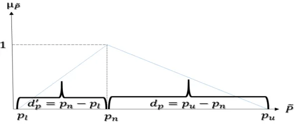
In some FLP methods, a certain number replaces the fuzzy one in the model. Peidro et al. (2009) suggested the replacement of certain value
3
′ −
+ p p
n
d d
p instead of triangular fuzzy number (TFN)
( , , )
= l n u
P% p p p shown in Fig. 2. We first generalize this method and then, apply the proposed method to defuzzify.
Figure 2. Triangular fuzzy number
Let the function
ϕ
:TFN →، be defined in the following form:( , , ) ( )
3
l n u
l n u
P p p p TFN
p p p
P
ϕ
= ⊆
+ +
=
(40)
According to Eq. (41), function
ϕ
has been used in the method of (Peidro et al., 2009) for defuzzification. Therefore, they replace the mean of components instead of TFS.(
) (
)
3
3
3
p p u n n l l n u
n n
d
d
p
p
p
p
p
p
p
p
+
−
′
=
p
+
−
−
−
=
+
+
(41)We define function
ϕ
λas follows:. ( ( , , ))
3 ( 1)
l n u
l n u
p p p
P p p p
λ
λ
ϕ
λ
+ +
= =
+ −
(42)
It is clear that function
ϕ
λ , contrary to functionϕ
, takes into consideration the weightλ
for the TFN nominal valuep
n. In this new defuzzification method, we can analyze the effect of nominal values on the results. Note that ifλ
=
1
, then we refer to the previous method.Note that the problem is defined in a fixed network. Therefore, the model size (the number of variables and constraints) depends on the cardinality of the index sets. Before defuzzification, the number of variables and constraints is formulated, respectively, as follows
:
| | (4 | | 5 | | 3 | | (| | | |) 4 | | | | 3 | || | 3 | |(| | | |)
3| |(| | | |)| | 3| || || |)
f d
f d
f d
T W WP PU C C W WP
WP PU PU C C
PU C C PL
WP PU PL
+ + + + +
+ + +
+ +
+ (43)
| | (3 | | 3 | | 2 | | (| | | |) 4 | | | | 2 | || | 3 | |(| | | |)
2| |(| | | |)| | 2| || || | 7)
f d
f d
f d
T W WP PU C C W WP
WP PU PU C C
PU C C PL
WP PU PL
+ + + + +
+ + +
+ +
+ +
(44)
After the defuzzification, the size of the model is equal to the above formulas, since only TFN changes to a deterministic number in Eq. (42).
4- Model implementation
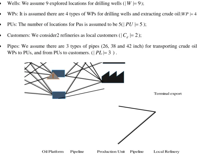
In this section, we investigate the application of the proposed model using the read data of Persian Gulf oilfields. The scales of the problem under investigation are as follows (see fig. 3):
• Wells: We assume 9 explored locations for drilling wells (|W| 9= );
• WPs: It is assumed there are 4 types of WPs for drilling wells and extracting crude oil|W P| 4= ;
• PUs: The number of locations for Pus is assumed to be 5(|PU| 5= );
• Customers: We consider2 refineries as local customers (
|
C
d| 2
=
);• Pipes: We assume there are 3 types of pipes (26, 38 and 42 inch) for transporting crude oil from WPs to PUs, and from PUs to customers. (|PL| 3= ) .
Figure 3. A schematic view of crude oil supply network in numerical study
4-1- Effects of time horizon on results
In this sub-section, the effects of the time horizon on the results are analyzed. The profitability of the activities are determined at the end of each period during 15-year time horizon, and at the end of each time horizon planning from 1-year to 15-year (Fig. 3).
Oil Platform Pipeline Production Unit Pipeline Local Refinery Terminal export
Usually, in strategic/long-time planning horizon,in the early planning, the profitability is lesser than short-time planning horizon. To clarify the subject, consider 7-year and 15-year planning horizons in which we want to determine NPV, and show the difference between short and long time horizons. Fig. 4 states that although, from the beginning to the end of the 8th year, NPV earned by the 15-year time
horizon is lesser than the value of the 7-year, conversely, from the 9th year to the end planning, NPV
earned by the 7-year time horizon is less than the values of the15-year, and the difference between them is enhanced. Thus, the length of the planning horizon problem has a significant impact on the decision-making.
Figure 4. NPV during time horizon planning
Figure 5. Trend of NPV during 7-year and 15-year time horizon planning
1 2 3 4 5 6 7 8 9 10 11 12 13 14 15 -200
0 200 400 600 800 1000
Time (year) NPV (million $)
NPV at the end of each period for 15-year horizon planning NPV at the end of each time horizon from 1-15 year
1 2 3 4 5 6 7 8 9 10 11 12 13 14 15
Time (year)
NPV at the end of each period during 15-year time horizon NPV at the end of each period during 7-year time horizon
Table1. NPV at the 1-15 time horizon, and NPV at the different period during 7-year and 15-year horizon planning
NPV (1 10× 6$) ; 15-year End of each time period NPV (1 10× 6$) ; 7-year
End of each time period NPV (1 10× 6$)
End of each time horizon Year -37.06 -20.88 0 1 80.87 92.29 170.92 2 190.55 209.31 253.43 3 330.62 338.42 452.18 4 420.58 452.50 500.90 5 520.20 578.08 593.97 6 593.74 674.27 674.27 7 675.47 730.80 752.11 8 761.23 753.02 794.25 9 790.84 793.62 841.40 10 870.19 834.73 900.59 11 905.22 860.48 922.26 12 930.17 873.57 954.60 13 955.22 891.23 962.71 14 965.22 903.74 965.22 15
4-2- Effect of “price and demand” on results
With regard to the economic point of view, price and demand are two important parameters in decision-making. We want to analyze the simultaneous effects of price and demand when they have their critical values (i.e. pl andpu). So, the results should be presented in the following four critical scenarios:
Scenario 1 2 3 4
Condition u u
price
p
demand
p
=
=
u lprice
p
demand
p
=
=
l uprice
p
demand
p
=
=
l lprice
p
demand
p
=
=
The effect of the mentioned scenarios on oilfield development can be calculated by different criteria. Suppose the situation of an oilfield is specified based on two criteria: one shows the “percent development
(PD)” and the other indicates the “percent production (PP)”. We define PD as the ratio of the available facilities (WPs, PUs, pipelines, etc.) to the minimum facilities required for full production while PP is defined as total production to the estimated capacity production from the beginning of development. Table 2 shows the results of the effects of price and demand on these two criteria at the end of the 15-year time horizon planning.
Table 2. The values of oilfield development criteria in critical scenarios
PP (%) PD (%)
Located PUs Installed WPs
Drilled wells
95.50 100
4 3
9 Scenario 1
70.00 81.33
4 2
8 Scenario 2
71.33 73.75
4 2
7 Scenario 3
40.13 43.66
2 1
5 Scenario 4
4-3- Effects of uncertainty on results
As mentioned in the previous section, due to existent uncertainty in data, TFNs are consider for model parameters. Obtained fuzzy optimization problem is transformed to deterministic model by function
ϕ
λ, and then solved by CPLEX solver.For different values of
λ
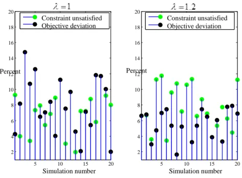
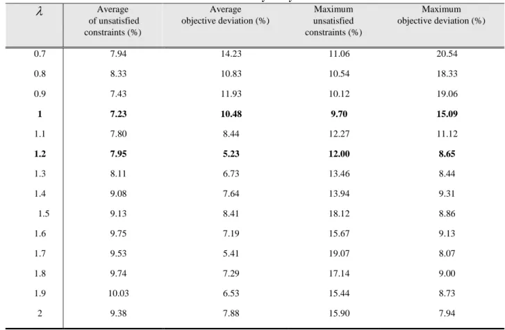
different deterministic models and, hence, different optimal solutions (SOL*λ) are possible. Suppose the real deterministic model is known; substituting every SOL*λ in it, some constraints may be unsatisfied and the objective function value may deviate from its optimum. Therefore, “percent of unsatisfied constraint” and “percent of deviation from the optimal objective function” are introduced as two criteria for the validation of theSOL*λ. But, since the deterministic model does not exist, several such models are simulated through considering membership functions of the fuzzy parameters, and the mentioned criteria are calculated for every one of them. It is obvious that the solution with average values less than those of the two criteria, is more reliable and its decision risks are less.We first simulate 20 certain models using membership function of TFNs, and then calculate the average of mentioned criteria. Computational results are tabulated in Table 3. Also, the value of criteria for
λ
=
1
andλ
=
1.2
is shown in Fig. 5 for every simulation.Figure 6. The value of Constraint unsatisfied and objective deviation criteria for
λ
=
1
andλ
=
1.2
5 10 15 202 4 6 8 10 12 14 16 18 20
Simulation number Percent
Constraint unsatisfied Objective deviation
5 10 15 20 2
4 6 8 10 12 14 16 18 20
Simulation number Percent
Constraint unsatisfied Objective deviation
Table 3. Sensitivity analysis of
λ
Maximum objective deviation (%) Maximum
unsatisfied constraints (%) Average
objective deviation (%) Average of unsatisfied constraints (%)
λ
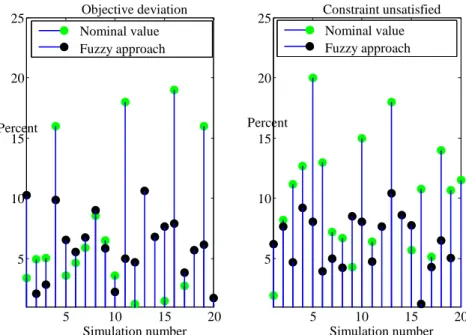
20.54 11.06 14.23 7.94 0.7 18.33 10.54 10.83 8.33 0.8 19.06 10.12 11.93 7.43 0.9 15.09 9.70 10.48 7.23 1 11.12 12.27 8.44 7.80 1.1 8.65 12.00 5.23 7.95 1.2 8.44 13.46 6.73 8.11 1.3 9.31 13.94 7.64 9.08 1.4 8.86 18.12 8.41 9.13 1.5 9.13 15.67 7.19 9.75 1.6 8.07 19.07 5.41 9.53 1.7 9.00 17.14 7.29 9.74 1.8 8.73 15.44 6.53 10.03 1.9 7.94 15.90 7.88 9.38 2In order to validate the proposed fuzzy method, again 20 certain models are simulated using membership function of TFNs. We compare SOL*λ=1.2 withSOL*Nominal, in which SOL*Nominal is optimum solution which is obtained by replacement nominal values instead of TFNs. As is clear from Fig. 6, although both solutions have approximately equal value in average, the deviations and risk of
* SOL
Nominal is very greater than *
1.2
SOLλ= . So, computational tests using randomly generated data are presented showing that the fuzzy approach is worth considering in these types of problems.
Figure 7. The compression of fuzzy approach (SOL*λ=1.2) and nominal value approach (SOL*Nominal)
5- Conclusions
In this work, we presented a mathematical programming model for the design of crude oil supply chain and planning of offshore oilfields development. The proposed model is a multi-period mixed-integer linear program which accounts for the optimization of the economic performance. The developed model considers the strategic decisions such as facility location (i.e., locations of wells and production units (PU)), facility allocation (i.e., assigning the wells to the PUs, and the PUs to the customers), and technology selection with respect to the capacity and cost. The tactical decisions include the optimal time for drilling, installation of the equipment facilities required for the production and transportation, optimal extraction of each well, and the amount of optimal production.
The application of the proposed model was examined through a case problem in which the real data of Gulf Oilfields and Iranian South Oilfields was utilized. In order to validate the performance of the fuzzy optimization model, some random problems were simulated using membership functions. We showed the proposed fuzzy formulation was more effective than the deterministic model in handling the real situations, where certain information is not available for the oilfield development planning. Furthermore, the fuzzy model did not result in an excessive computational time. Additionally, we analyzed the effects of the time horizon on the results. Our computational results implied the length of the planning horizon has a significant impact on the decision-making. The obtained results, in addition, revealed that a long time horizon could provide a larger NPV at the end of the oilfield Life-cycle.
For the future work, it would be interesting to investigate the nonlinearity behaviors of the oil reservoirs, the pressure drops of the oil wells, and the impacts of the activities on the environment and society.
5 10 15 20
5 10 15 20 25
Simulation number Percent
Objective deviation Nominal value Fuzzy approach
5 10 15 20
5 10 15 20 25
Simulation number Percent
Constraint unsatisfied Nominal value Fuzzy approach
References
ASEERI, A., GORMAN, P. & BAGAJEWICZ, M. J. 2004. Financial Risk Management in Offshore Oil Infrastructure Planning and Scheduling. Industrial & Engineering Chemistry Research, 43, 3063-3072.
BELLMAN, R. E. & ZADEH, L. A. 1970. Decision-Making in a Fuzzy Environment. Management
Science, 17, B-141-B-164.
CARVALHO, M. C. A. & PINTO, J. M. 2006a. A bilevel decomposition technique for the optimal planning of offshore platforms. Brazilian Journal of Chemical Engineering, 23, 67-82.
CARVALHO, M. C. A. & PINTO, J. M. 2006b. An MILP model and solution technique for the planning of infrastructure in offshore oilfields. Journal of Petroleum Science and Engineering, 51, 97-110. DAMGHANI, R. K. V. R. G. K. K. 2015. Optimization of multi-product, multi-period closed loop supply
chain under uncertainty in product return rate: case study in Kalleh dairy company. Journal of Industrial and Systems Engineering.
DEVINE, M. D. & LESSO, W. G. 1972. Models for the Minimum Cost Development of Offshore Oil Fields. Management Science, 18, B-378-B-387.
GUPTA, V. & GROSSMANN, I. E. 2012. An Efficient Multiperiod MINLP Model for Optimal Planning of Offshore Oil and Gas Field Infrastructure. Industrial & Engineering Chemistry Research, 51,
6823-6840.
GUPTA, V. & GROSSMANN, I. E. 2014. Multistage stochastic programming approach for offshore oilfield infrastructure planning under production sharing agreements and endogenous uncertainties. Journal of Petroleum Science and Engineering, 124, 180-197.
HENNIG, F., NYGREEN, B., CHRISTIANSEN, M., FAGERHOLT, K., FURMAN, K. C., SONG, J., KOCIS, G. R. & WARRICK, P. H. 2012. Maritime crude oil transportation – A split pickup and split delivery problem. European Journal of Operational Research, 218, 764-774.
IYER, R. R., GROSSMANN, I. E., VASANTHARAJAN, S. & CULLICK, A. S. 1998. Optimal Planning and Scheduling of Offshore Oil Field Infrastructure Investment and Operations. Industrial & Engineering Chemistry Research, 37, 1380-1397.
KOSMIDIS, V. D., PERKINS, J. D. & PISTIKOPOULOS, E. N. 2002. A Mixed Integer Optimization Strategy for Integrated Gas/Oil Production. In: JOHAN, G. & JAN VAN, S. (eds.) Computer Aided Chemical Engineering. Elsevier.
KOSMIDIS, V. D., PERKINS, J. D. & PISTIKOPOULOS, E. N. 2004. Optimization of Well Oil Rate Allocations in Petroleum Fields. Industrial & Engineering Chemistry Research, 43, 3513-3527. LIU, B. 2010. Uncertainty Theory. Uncertainty Theory. Springer Berlin Heidelberg.
PEIDRO, D., MULA, J., POLER, R. & VERDEGAY, J.-L. 2009. Fuzzy optimization for supply chain planning under supply, demand and process uncertainties. Fuzzy Sets and Systems, 160, 2640-2657.
RIBAS, G., LEIRAS, A. & HAMACHER, S. 2011. Tactical planning of the oil supply chain: optimization under uncertainty. PRÉ-ANAIS XLIIISBPO.
SAHEBI & NICKEL 2014. Offshore oil network design with transportation alternatives. European Journal of Industrial Engineering, 8.
SAHEBI, H., NICKEL, S. & ASHAYERI, J. 2014. Strategic and tactical mathematical programming
models within the crude oil supply chain context—A review. Computers & Chemical
Engineering, 68, 56-77.
SHAH, N. K., LI, Z. & IERAPETRITOU, M. G. 2011. Petroleum Refining Operations: Key Issues, Advances, and Opportunities. Industrial & Engineering Chemistry Research, 50, 1161-1170. SHAMS, H., MOGOUEE, M. D., JAMALI, F. & HAJI, A. 2012. A Survey on Fuzzy Linear
Programming. American Journal of Scientific Research, 117-133.
SHEN, Q., CHU, F. & CHEN, H. 2011. A Lagrangian relaxation approach for a multi-mode inventory routing problem with transshipment in crude oil transportation. Computers & Chemical Engineering, 35, 2113-2123.
TANAKA†, H., OKUDA, T. & ASAI, K. 1973. On Fuzzy-Mathematical Programming. Journal of Cybernetics, 3, 37-46.
TARHAN, B., GROSSMANN, I. E. & GOEL, V. 2009. Stochastic Programming Approach for the Planning of Offshore Oil or Gas Field Infrastructure under Decision-Dependent Uncertainty.
Industrial & Engineering Chemistry Research, 48, 3078-3097.
TSARBOPOULOU, C. 2000. Optimization of oil facilities and oil production. Optimisation of Oil Facilities and Oil Production.
VAN DEN HEEVER, S. A. & GROSSMANN, I. E. 2000. An Iterative Aggregation/Disaggregation Approach for the Solution of a Mixed-Integer Nonlinear Oilfield Infrastructure Planning Model.
Industrial & Engineering Chemistry Research, 39, 1955-1971.