A BINOMIAL MODEL APPROXIMATION FOR
MULTIPLE TESTING
1I. A. ADELEKE, 2A. O. ADEYEMI AND 2E. E. E. AKARAWAK
1Department of Actuarial Science and Insurance, University of Lagos, Nigeria.
2Department of Mathematics, University of Lagos, Nigeria.
*Corresponding Author: [email protected], Tel +2348035648121
values ( or p – values (Holm, 1979); Westfall and Young, 1989, 1993. Hocheberg, 1988, and Hommel, 1988. Recently, (de Una-Alvarez, 2015) developed a new BB-SGoF method for comparing the procedures in multiple testing using SGoF package.
The standard Bonferroni adjustment proce-dure, which is very popular for multiple tests posits that if any of the test in (n) multiple test has the hypothesis should be rejected (Savitz and Olshan, 1995). The ma-jor problem of this Bonferroni procedure is that it has the tendency of increasing the probability of producing false negatives which is a reduction in statistical power of rejecting H0 in each test conducted (Nakagawa, 2004). Sidak (1967) procedure
ABSTRACT
Multiple testing is associated with simultaneous testing of many hypotheses, and frequently calls for adjusting level of significance in some way that the probability of observing at least one significant result due to chance remains below the desired significance levels. This study developed a Binomial Model Approximations (BMA) method as an alternative to addressing the multiplicity problem associat-ed with testing more than one hypothesis at a time. The proposassociat-ed method has demonstratassociat-ed capacity for controlling Type I Error Rate as sample size increases when compared with the existing Bonferroni and False Discovery Rate (FDR).
Keywords: Bonferroni Procedure, False Discovery Rate, Binomial Model Approximation, False Posi-tives, False NegaPosi-tives, Multiple Testing
INTRODUCTION
Multiple testing is a statistical technique of performing simultaneous multiple test of hypothesis. The multiplicity problem associ-ated with simultaneous testing of many hy-potheses is the basis of multiple testing; it is an error rate controlling issue. Application of multiple testing gained widespread popu-larity in health services research among bio-statisticians, medical biologists and pharma-ceutical industries. Multiple testing has been of great research interest in Statistics and researchers are searching for various scien-tific methods to improve the existing proce-dures in multiple testing. Consequently, many methods have been developed in liter-ature for multiple testing. Most of the meth-ods are developed from the parameter Bon-ferroni inequality for adjusting significance
Journal of Natural Science, Engineering
and Technology
ISSN:
Print - 2277 - 0593 Online - 2315 - 7461
was developed to test each hypothesis at with accuracy better than the Bonferroni; however the gain in power is small. Holm (1979) introduced the se-quential Bonferroni procedure to counter-act the problem of power reduction. Alt-hough this procedure still exhibits power reduction, it is in low extent (Nakagawa, 2004). Holm (1979) applied the Sequential Bonferroni method for multiple adjust-ments and the approach was used to con-trol the family-wise Type I error rate, the flexibility of the approach when compared to the Bonferroni correction makes Holm’s to be more popular among researchers. Hocheberg, (1988) also improved on the Bonferroni method with stepwise adjust-ments for adjusting p-value sequentially while making sure the observed p-value or-der was preserved. The improved procedure rejects all hypotheses with smaller or equal p-value to that of any p-values discovered to be smaller than its critical value. The method is a step up procedure sharper than the sequentially rejected procedure of Holm (1979). Gaetano (2013) extended the Holm sequential Bonferroni procedure and intro-duced an Excel calculator for calculating the sequential corrected p-values. The first study of stability properties of the Bonfer-roni and Benjamini-Hochberg (BH) proce-dures shows that the extended Bonferroni procedure can be made as powerful as the BH procedure by a proper choice of its pa-rameter (Gordon et.al. 2007). The work of Dunnett and Tamhane (1992) which has not been implemented in any statistical soft-ware was also developed as a stepwise pro-cedure for controlling type II error rate ac-cording to (Blakesley et al., 2009). Dunnett and Tamhane (1992) is a step-up procedure for comparing k treatments with a control, the study revealed that the step-up is often
more powerful than the single–step and the step-down procedures.
The False Discovery Rate (FDR) was sug-gested by Benjamini and Hochberg (1995) as an alternative procedure. It has been ob-served by (Benjamini et al. 2001) that FDR is the expected proportion of false discoveries among the discoveries, and controlling the FDR goes a long way towards controlling the increased error from multiplicity while losing less in the ability to discover real differences. In a study of multivariate samples involving analysis of large micro array data, instead of using Bonferroni Corrections, Garcia (2003) applied FDR controlling the error rate. Sto-rey (2003) described FDR as an error meas-ure mechanism in multiple hypothesis test-ing; it is an expected proportion of false pos-itives among all significant proportions of hypothesis. The researcher introduced and investigated pFDR, and q-value; the pFDR is a
modified FDR while q-value is the pFDR
analogue of the p-value.
The method of Binomial Model Approxima-tion (BMA) for multiple testing is introduced in this paper. The proposed method has been compared with some multiple testing procedures in the literature using computer simulation. The remainder of this article is as follows. Section 2 presents the materials and method; section 3 presents the proposed Bi-nomial Model Approximation method. In section 4, results are discussed while section 5 concludes the paper.
MATERIALS AND METHOD
The BMA technique is a generalization of the Bernoulli experiment with n number of hypothesis, the method satisfies the condi-tions for a discrete probability function f(x) >0. The assumptions for the methodology are that;
There are n Hypothesis tests to be conduct-ed, the Hypothesis tests are independent, the probability of success (correctly reject-ing the true null Hypothesis) is α, the proba-bility of failure ( not rejecting the true null Hypothesis) is 1- α. and the probability of observing at least one significant result due to chance occurrence is:
P (A) =1-P (B) = Where P(A) is the probability of obtaining
at least one significant result and P(B) is the probability of no significant result.
The method requires setting up the null and alternative hypotheses Ho and Ha re-spectively, the test procedures and selection of significance level (α). The test statistics and its associated values are calculated and used in making decision about the null hy-pothesis.
In a test involving only two hypotheses, the parameters of two mean vectors for the test can be estimated using the Hotelling T square method.
The sample mean vectors are:
and
The estimated variances are
Both Sx and Sy are estimators for the common variance-covariance matrix Σ.
Multiple testing: In multiple testing, using
at least one procedure, the methodology required that for one or more false discov-ery among the null hypothesis, the global null hypothesis is rejected. Using none or all procedure required that for false discovery among all the null hypotheses, the global null hypothesis is rejected.
In a multivariate analysis of multiple sam-ples divided into groups A and B, the ex-periment required many hypotheses to be tested. The multivariate variables (X, Y) are
designed in form of data matrix such that: observation in the data frame X
and observation in the data
frame Y, i=1,2…n rows, j=1,2…m columns. In carrying out n-multiple tests simultane-ously, the estimated sample mean and its var-iance from samples in population group A is:
Multiplicity Adjustment in Multiple Testing
Adjustment for multiplicity is very crucial and requires topmost attention most espe-cially in clinical trials, this is because it tends to inflate the Type I error rate of the experi-ment. In order to mitigate this multiplicity problem of incorrectly rejecting a true null hypothesis, statisticians have developed sev-eral multiple comparison adjustment proce-dures. Multiplicity adjustment involved ei-ther
(i) Adjusting significance levels (α)
down-ward or (ii) Adjusting p-values for Hi, the
lowest overall error rate (α) at which the hy-pothesis is rejected.
Some of the existing procedures in literatures are:
Bonferroni Correction
The standard Bonferroni adjustment proce-dure states that if any of the multiple tests has the hypothesis should be re-jected.
,
The associated variance-covariance matrix is
.
The null and alternative hypotheses for the multiple sample tests is presented respectively as,
Mean of the k – observations in sample m,
gFWER controlling method
At significance level α, assume we have F as the number of false positive and t as the number of rejected null hypothesis.
is the generalized family-wise error rate (gFWER). It means rejecting t more hypotheses at controlling level α of the gFWER. It is the probability of errone-ously rejecting at least one true null hypoth-esis.
Benjamin-Hochberg (BH) method
Let G be any number of rejected hypothe-ses at α while F is the number of false
posi-tives.
The FDR is defined as the ratio of the num-ber of Type I errors by the numnum-ber of sig-nificance tests.
Instead of controlling the overall alpha lev-el, Benjamin –Hochberg proposed a proce-dure for controlling the False Discovery Rate (FDR)
The Holm-Bonferroni (HB) Procedure
This procedure is based on Holm’s paper of 1979; it is a modification from the existing Bonferroni approach.
The procedure runs a test for each hypothe-sis to obtain their p-values; the p-values are then compared to the calculated Holm-Bonferroni for the specific hypothesis or-dered from smallest to greatest.
In a multiple testing of n hypothesis ,
…. with corresponding ,
…
Giving FWER at alpha level=0.05
HB is calculated for the starting from the smallest
Any whose is significant
and the null hypothesis is rejected.
BB-SGoF Procedure
de Una–Alvarez (2015) proposed a beta-binomial model, a correction of SGoF for serially dependent tests. The Beta-Binomial transforms the original p-values and assumes independent blocks of p-values. Each block is chosen to be a realization of beta-binomial variable introduced as a suitable modification of the sequential goodness-of–fit multiple In testing , i=1,2…n hypothesis, is rejected if
testing techniques having correlated blocks, the Beta distribution is the Bayesian prior of parameter
The procedure was applied to two different real data sets, the study revealed that BB-SGoF method weakly controls for FDR. The authors concluded that the SGoF pro-cedure may have much power even when
there is possibility of dependences among the tests to be carried out.
THE BINOMIAL MODEL
APPROXIMATION METHOD
In this study, the BMA procedure was intro-duced to calculate adjusted probabilities us-ing the Z score.
In order to test the following hypothesis
The threshold value (α) of the Hypothesis is defined together with the associated p-value
From equation 3.1, when α = 0; the Probability of at least one significant result = 0, also
when
α = 1; Probability of at least one significant result = 1
Table 1. Outcome of Binary Trials
Α P(A) <α
0 0
1 1
When the p-value is less than α, (p <α) the result is said to be statistically significant at the level α.
The experiment is transformed as a binomi-al model experiment involving a binary event of success or failure, correctly reject-ing hypothesis or incorrectly rejectreject-ing hy-pothesis.
From equation 3.1 and the table above, n is the total number of hypothesis while is
the parameter of the Binomial Model, (0 < < 1). The number of true null hypothesis denoted as x can be chosen from n total hypothesis in ways.
Under this method, is defined as the probability of success and (1- ) is defined as the probability of failure.
The empirical null hypothesis is an estimat-ed distribution for the test statistics under the null hypotheses when the test statistics can no longer be considered as a random sample from the theoretical null distribu-tion. The adjusted p-value is used for taking decision on the true null hypothesis which is rejected whenever p-value is less than ad-justed p-value.
Multiple testing in the field of biostatistics and clinical trials is a big data challenge in large microarray data. As n (the number of tests) increases, Binomial Model can be ap-proximated using the normal distribution. The binomial distribution by the Central Limit Theorem approximates to the standard
normal distribution as n→infinity. ),
is approximately ;
nα is the mean and the standard deviation is
P(Type I error) = number of False/ (number of True+ number of False), is the number of False Positives i.e when we false-ly reject the null Hypothesis when P(X ≥
x0 - 0.5)
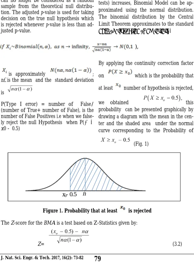
By applying the continuity correction factor
on which is the probability that
at least number of hypothesis is rejected,
we obtained this
probability can be presented graphically by drawing a diagram with the mean in the cen-ter and the shaded area under the normal curve corresponding to the Probability of
(Fig. 1)
nα
x0- 0.5
Figure 1. Probability that at least is rejected
The Z-score for the BMA is a test based on Z-Statistics given by:
The Statistics is compared with the value from the Z-Table under the following hy-pothesis.
RESULTS
Method of Simulation: 50,000 random data sets were generated with two groups, of
40,000 and 10,000 observations for Type I and Type II errors respectively. The samples were used to estimate false positive and false negatives.
The table below is a result of the simulation carried out on different methods of multiple comparisons in the literature. The R software was used for the analysis to generate proba-bility for the false negative and false positive.
Table 2. Results of Computer Simulation Comparing Various Methods Procedures False Positive
TYPE 1 ERROR=
FALSE/TRUE + FALSE
False Negative TYPE II ERROR= TRUE/TRUE + FALSE
Binomial Model Approximation
2055/40,000 = 0.0514 9488/10,000 = 0.9488
Bonferroni 0/40,000 = 0.0000 10,000/10,000 = 1.0000
False Discovery Rate 453/40,000 = 0.0113 9891/10,000 = 0.9891
Benjamini-Hochberg 2055/ 40,000 = 0.0514 9488/10,000 = 0.9488
Benjamini-Yekutieli(BY) 2055/ 40,000 = 0.0514 9488/10,000 = 0.9488
Hommel Approach 2055/ 40,000 = 0.0514 9488/10,000 = 0.9488
Holm Procedure 2055/ 40,000 = 0.0514 9488/10,000 = 0.9488
Hochberg method 2055/ 40,000 = 0.0514 9488/10,000 = 0.9488
DISCUSSION
Increase or decrease in the false negatives versus false positive depends on the nature of the problem and consequences of each type of error. Different methods were used to compute the type I error and type II er-ror rates, the result of the method proposed was compared with other methods obtained in the existing literatures.
From the summary of simulation using R software, all the procedures apart from FDR, and BONFERRONI have the same
return values of false positives and false neg-atives. This implies the procedures have the ability to limit the probability of incorrectly rejecting the null hypothesis. It also reveals that the BMA has the ability to control the Type I error, the central limit theorem guar-antees that the result is equivalent under nor-mal sampling for large testing.
Some of the literature advised that it is al-ways good to use a procedure which is more familiar to the researchers and more applica-ble to the specific field of study. In
particu-lar, taking a decision on the effectiveness of new drugs over the existing ones require high degree of accuracy, therefore, proce-dures that can help in effectively controlling the probability of committing type I error relative to type II error should be adopted. A type I error occurs when we falsely reject the null hypothesis while a type II error oc-curs when we erroneously failed to reject the null hypothesis, i.e. when there is a fail-ure to detect a difference.
CONCLUSION
FDR based method aimed to control ex-pected proportion of false discoveries at a given (α), in this situation, the BH and BY are suggested useful methods for independ-ent and dependindepend-ent test respectively. The Bonferroni Correction is appropriate when false positive in a set of tests would be a problem. When there are a large number of testing, i.e. (as the testing increases), and the researcher is interested in much likely significance, the Bonferroni Correction leads to a very high rate of false negatives. This has also been confirmed in this study as revealed in the Bonferroni probability of Type II error =1, showing the maximum rate of false negatives. As the number of testing increases this study has shown that the Binomial Model Approximation (BMA) is adequate.
The study agrees with the view of Castro-Conde and de Una-Alvarez (2015) who concluded in their work that even though FDR based method are often used nowa-days to take multiplicity of tests into ac-count, they may exhibit poor power in some particular scenario when the number of test is large, therefore application of al-ternative method is recommended.
REFERENCES
Benjamin et al. 2001. Controlling the false
discovery rate in behavior genetics research. Behavioural Brain Research 125(1-2):279-84.Doi:10.1016/s0166-4328(01)00297-2.
Benjamini., Hochberg 1995. Controlling
the False Discovery Rate: A Practical and Powerful Approach to Multiple Testing. Jour-nal of the Royal Statistical Society, series B (methodological), Vol.57,NO.1, 289-300
Blakesley R.E., Mazundar, S; Dew, M.A; Houck P.R Tang G., Reynolds, C.F; and Butters, M.A. 2009 .Comparisons of
meth-ods of multiple hypotheses testing in Neuro-psychological Research. Neuropsychology 23(2) 255 -264 http://doi.org/10.1037/a0012850 PMCID, PMC 3045855
de Una-Alvarez J. 2015. The Beta-Binonual
SGoF method for multiple dependent tests, Statistical Application in Genetics and Molecular Biology, 11(3), 198-106
Dunnett., Tamhane. 1992. Calculation of
critical values of Dunnet and Tamhane’s Step-up Multiple Test Procedure. Journal of America Statistical Association, 87, 162-170.
Gaetano J. 2013. Holm-Bonferroni
sequen-tial correction: An Excel calculator (1.1) doi:10.13140/RG.2.1.4466.9927
Garcia L.V, 2003. Controlling the false
dis-covery rate in ecological research. Trends in Ecology and Evolution. 18: 553 -554.
Gordon. A., Glazko. G., Qiu. X., Ya-kovlev. A. 2007. Control of The Mean
Number of False Discovery, Bonferroni and Stability of Multiple Testing. Anals of Applied Statistics. Volume 1, Number 1, 179-190, Doi:10.1214/07-A0AS102
Hochberg, Y. 1988. A sharper Bonferroni
procedure for multiple tests of significance. Biometrika 75(4): 800-802. https:// doi.org/10.093/biomet/7.
Holm. S. A. 1979. A simple sequentially
rejective multiple test procedure. Scandina-vian Journal of statistics, 6, 65-70.
Hommel, G.A. 1988. A stagewise rejective
multiple test procedure based on a modified Bonferroni test. Biometrika. 75: 383-386.
Peter H Westfall., S. Stanley Young.
1989. P-value Adjustment for multiple tests inMultivariate Binomial Models. Journal of the American statistical association 84(407): 780-789.
Savitz DA., Olshan AF. 1995. Multiple
Comparison and Related Issues in the Inter-pretation of Epidemiologic data. Am J
Epi-demiol. 142: 904-908.
Shinichi Nakagawa. 2004. A farewell to
Bonferroni: The problems of low statistical power and publication bias. Behavioural Ecolo-gy 15(6): 1044- 1045.
Sidak Z. 1967. Rectangular confidence
re-gions for the means of multivariate normal distribution. Journal of the American Statistical A s s o c i a t i o n . 6 2 ( 3 1 8 ) : 6 2 6 - 6 3 3 , doi:10.1080/01621459.1967.10482935.
Storey, J.D. 2003. The positive false
discov-ery rate. A Bayesian interpretation and the q-values. The annals of statistics 31(6): 2013-2035.
Westfall., Young. 1993. Resampling-Based
Multiple Testing: Examples and Methods for p-value Adjustment. ISBN: 978-0-471-55761-6