1076.pdf

CONTENTS

Acknowledgements ... 11

Abstract ... ill List of figures ... iv

List of tables ...v

Introduction... 1

Literature review ... ... 4

Analytical techniques ... 4

Radon hazard ... 6

Radon in groundwater... 12

Geological influence ... 15

Materials and methods ... 18

Emanation... 19

Liquid scintillation ... 26

Calibrations ... 27

Data analysis ... 30

Calibration factors ... 30

Exploratory data analysis ... 35

Hypothesis testing ... 40

Liquid scintillation precision ... 54

Lower limit of detection ... 59

Quality control ... 60

Conclusions ... 63

Appendices I ... 66

II ... 67

III ... 70

IV... 72

References ... 75

Acknowledgements

I would like to express special thanks to my research advisor Dr. James Watson for his guidance and suggestions,

especially during the writing of this report. He has spent

many hours reviewing this document as it progressed through

several revisions. I would also like to thank Dr. Douglas

Crawford-Brown for his assistance with the scintillation cell counting system, the liquid scintillation counting

system and for serving as a committee member for my oral

presentation. Thanks also to Dr. Alvis Turner for serving

Abstract Kenneth Ladrach THE OCCDRRENCE OF RADON

IN SOME NORTH CAROLINA GROUNDWATER SUPPLIES (Under the direction of Dr. James E. Watson)

Approximately one hundred small public groundwater sup¬

plies in North Carolina were sampled. Analyses for

radon-222 were performed by two methods, emanation and a

newer liquid scintillation counting (LSC) method. Two

primary goals were involved in this work, (1) comparing the

two analysis methods listed above and (2) testing for an

association between radon concentration in groundwater and

the geology of the sampled site. The data show

statistically significant differences in radon

concentrations measured by the two methods. In 75 percent

of the cases the liquid scintillation result was lower,

indicating the possible need for refinement of this

technique. The precision of liquid scintillation results

was tested by comparing dual samples from each site. A

paired difference T-test on the dual LSC measurements

indicates that the mean difference between dual LSC

measurements is equal to zero. Forty three of fifty two

differences are less than 10 percent different. The radon

concentration data show in general, higher radon

concentrations associated with granite and gneiss/schist

rock formations over those in mafic and metavolcanic

formations. Samples from the coastal plain area had the

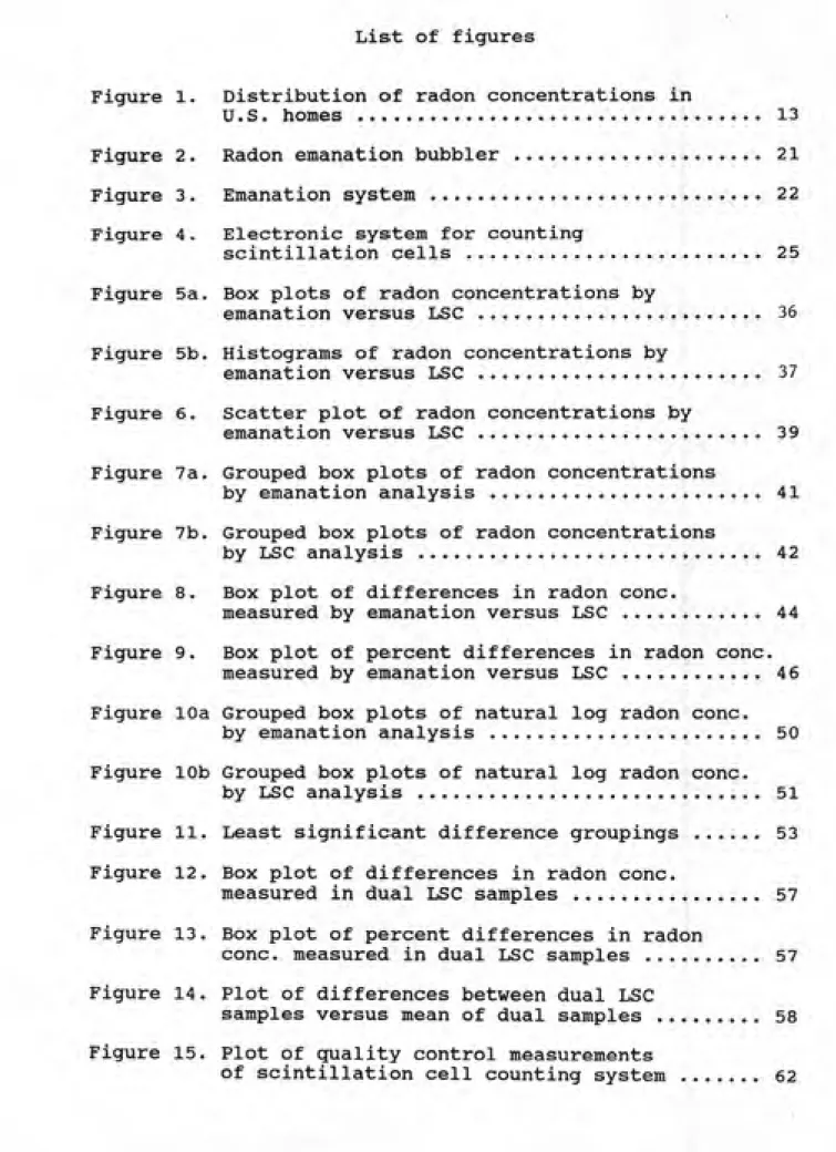
List of figures

Figure 1. Distribution of radon concentrations in

U.S. homes ... 13

Figure 2. Radon emanation bubbler ... 21

Figure 3. Emanation system ... 22

Figure 4. Electronic system for counting

scintillation cells ... 25

Figure 5a. Box plots of radon concentrations by

emanation versus LSC ... 36

Figure 5b. Histograms of radon concentrations by

emanation versus LSC ... 37 Figure 6. Scatter plot of radon concentrations by

emanation versus LSC ... 39

Figure 7a. Grouped box plots of radon concentrations

by emanation analysis ... 41

Figure 7b. Grouped box plots of radon concentrations

by LSC analysis ... 42

Figure 8. Box plot of differences in radon cone.

measured by emanation versus LSC ... 44

Figure 9. Box plot of percent differences in radon cone.

measured by emanation versus LSC ... 46

Figure 10a Grouped box plots of natural log radon cone. by emanation analysis ... 50

Figure 10b Grouped box plots of natural log radon cone.

by LSC analysis ... 51

Figure 11. Least significant difference groupings ... 53

Figure 12. Box plot of differences in radon cone.

measured in dual LSC samples ... 57

Figure 13. Box plot of percent differences in radon

cone, measured in dual LSC samples ... 57

Figure 14. Plot of differences between dual LSC

samples versus mean of dual samples ... 58

Figure 15. Plot of quality control measurements

Table 1. Summary of lung dose equivalents ... 7

Table 2. Lifetime lung cancer risks per pCi/m-' ... 10

Table 3. Lifetime lung cancer risks per WLM per year... 10

Table 4. Calibrations obtained at UNC with source

from interlaboratory study ... 32

Table 5. Calibration results from participants in

interlaboratory study ... 33

Table 6. Calibrations obtained with source from

the EPA, Las Vegas, Nevada ... 34

Table 7. Analysis of variance tables ... 52

Table 8. Radon concentrations measured in

sented in this technical report. The first question this

report addresses is whether two methods used in the

Radiological Hygiene Laboratory to measure radon

concentrations in water samples provide comparable results.

The standard procedure of emanating radon from a glass

sample collection bubbler into an alpha scintillation cell

for counting (Lucas 1957) has been used by a number of

researchers in the past (APHA 1976, Lee 1979, Michel 1980,

Mitsch 1982). Previous work by Radiological Hygiene

students (Strain 1978, Mitsch 1982 and Hayes 1984) utilized

this type of equipment and procedures for emanation analyses

of groundwater samples from wells in the phosphate mining

region of eastern North Carolina. For the current project

the emanation apparatus and procedures were used to measure

radon concentrations in well water samples collected

statewide. However we wanted to implement an alternative

analytical technique that would be reasonably accurate,

reliable and less time intensive. The liquid scintillation counting method described by Prichard and Gesell (Prichard

1977) and subsequently used in a nationwide study (Horton

1983) seemed a good candidate. Sample collection for liquid

scintillation counting analysis is easy to perform but

analysis requires a liquid scintillation counter plus blank

and standard activity vials. Since a programmable liquid

needed. A synopsis of the procedures used by the

Environmental Protection Agency in their nationwide study of

radon in drinking water (Horton 1983) was obtained from

Larry Kanipe (personal communication, current address:

Tennessee Valley Authority, Muscle Shoals, Alabama 35660).

A good liquid scintillation counting procedure would provide

an excellent alternative to emanation because more samples

could be analyzed in a shorter period of time without

requiring the presence of someone to operate the equipment. An important question is whether the liquid scintillation

counting procedure performs accurately and reliably in

comparison to the emanation procedure. This is the reason for comparison of emanation and liquid scintillation

counting results in this report.

The second question this report is concerned with is

the distribution of radon concentrations in groundwater as a

function of different geological regions of the state. This

technical report examines radon concentrations in water

samples from well sites classified in five major geological

groups across North Carolina. A statistical test for

significant differences in radon concentrations between

geological groups is performed. The longer range goal of

this type of work is to be able to predict with confidence

the concentration of radon to be expected in a given

groundwater sample based on site geological characteristics

Analytical techniques

For years the standard analytical technique for the

determination of radon concentration in water has been

emanation of radon from the water into an evacuated

scintillation cell for counting (APHA 1985). More recently,

liquid scintillation counting (LSC) techniques have been

used to measure radon concentrations. For example, the air

in a cave in Japan was analyzed for radon by counting

scintillation fluid after bubbling air through it in a

scrubbing bottle (Amano 1985). In another study, thoron and

radon gas bubbling from a hot spring was collected in a

syringe, liquid scintillator was added and the mixture

transferred to a vial for counting (Yoshikawa 1986). Two

researchers used LSC in conjunction with other methods of

analysis to study radon concentrations in groundwater (Ohnuma 1982, Oliveira de Sampa 1980). Radon concentrations

measured by LSC were compared with concentrations measured

using an ionization chamber (Ohnuma 1982). The coefficient

of variation in LSC measurements was given as 4.9 percent

and the correlation between the two methods was given as

0.966 (Ohnuma 1982). Oliveira de Sampa (1980) fabricated

scintillation cells by internally lining the walls of

Erlenmeyer flasks with silver activated zinc sulfide.

Samples were then analyzed by emanation and LSC. Both

sample was reported to be lost by retention in the emanation

system and 95 percent of the radon in the sample was

reported to remain dissolved in the liquid scintillation

cocktail (Oliveira de Sampa 1980).

In a review of methods for radiological analyses of

drinking water, Blanchard (1985) cites four investigators

who have used LSC to determine radon concentrations (Noguchi

1964, Homma 1977, Prichard 1977 and Horton 1983). High

volume extraction of radon from water followed by LSC was

performed by Noguchi (1964) and Homma (1977). This technique was used to indirectly measure radium-226 in

environmental samples. Simplified procedures have been used

to directly measure radon in water collected in low volume samples using commercially available liquid scintillation

counters (Prichard 1977 and Horton 1983). Broad spectrum

energy windows were used by both investigators; however,

different scintillation cocktails were employed. The

precision of paired LSC measurements in the study by Horton

(1983) was assessed by plotting the average range between

paired measurements against average concentration. A linear

fit to the data produced a slope of 0.054, indicating about

5 percent degree of precision over the range of

concentrations measured. The accuracy of the LSC technique

was checked through participation in an interlaboratory

study at the University of Texas in Houston and a comparison

well with the known values of controls. For the comparison

study with USC, a set of ten samples was analyzed by LSC

(EPA-EERF lab) and by emanation (USC Geology lab). The

correlation between the two sets of measurements was 0.998.

The use data were found to be about 10 percent lower than

the EPA data as observed in a scatter plot of the two datasets. The LSC method used by the EPA (Horton 1983) was

used in this study for comparison with the emanation method

because of the ease of sampling and analysis as well as the

previously demonstrated measurement capabilities of the

technique.

In the remainder of the literature review the hazard of

radon exposure is described in terms of increased risk of

lung cancer induction, and a relationship is presented

between the hazard of indoor radon and the potential

contribution of radon in groundwater to this hazard.

Finally, the question of the influence of geology on the

radon content of groundwater is explored. Radon hazard

Radon gas and associated daughter products have been a

concern for some time. On the average, radon daughters

contribute the largest fraction of annual lung dose from all

the sources of natural background radiation (NCRP #45 1975 &

#77 1984), see table 1. In table 1 the category "inhaled

radionuclides" refers primarily to inhaled radon daughters.

inhala-Cosmic radiation

Cosmogenic radionuclides

External terrestrial Inhaled radionuclides

Radionuclides in the body

Rounded totals

28 1 26

450 ₍₃₀₀₀₎ 24

(40) •"

Allowing for 10% shielding by buildings.

Allowing for 20% shielding by buildings and 20% by the body.

Does not include thoron and its daughters. The modified value alloxv^s

for indoor exposure to radon daughter inhalation and a change in quality factor from 10 to 20 for alpha radiation.

Allows for a change in quality factor from 10 to 20 for alpha radiation.

Table 1. Summary of lung dose equivalents (in mrem/yr) from various

sources of natural background radiation. Doses are to the

Protection and Measurements studied the available data on

the effects of radon inhalation experiments involving

animals and data on the effects of radon inhalation among

underground uranium mine workers. Their examination of data

on effects of inhaling radon daughters found that animal

study results parallel epidemiological studies of mine workers inhaling radon daughters. Several important points

are made. First, very high cumulative exposures, over 1000 working level months (WLM), are less effective at lung

cancer induction per WLM than are more moderate cumulative

exposures. Secondly, the highest lung cancer risk

coefficients for humans (50 x lOE -6 lung cancers/yr/WLM)

were found among those exposed to radon daughters later in

their lives (NCRP #78 1984). Finally, the regions of the human lung receiving the greatest absorbed dose from radon

daughters are the basal cells of the epithelial tissue in

the upper airways of the tracheobronchial tree. In fact

human lung cancers do appear predominantly in the upper

airways of this region (NCRP #78 1984).

NCRP report #78 adopts an average lung cancer risk co¬

efficient of 10 X lOE -6 cancers/yr/person/WLM averaged over

all age and exposure groups. Through a time integrating

risk model NCRP converts this to a lifetime risk of about

1.5 X lOE -4 lung cancers per WLM averaged over all age and

exposure groups. This is comparable to a range given by the

cancers/yr/person/WLM as well as an exponential term to

account for the decrease in cancer appearance rate due to

cellular repair and cell death over time. NCRP #78 presents

tabulated lifetime lung cancer risks for environmental

3

levels of radon daughter exposure per pCi/m or per WLM per

year for different ages of first exposure and different

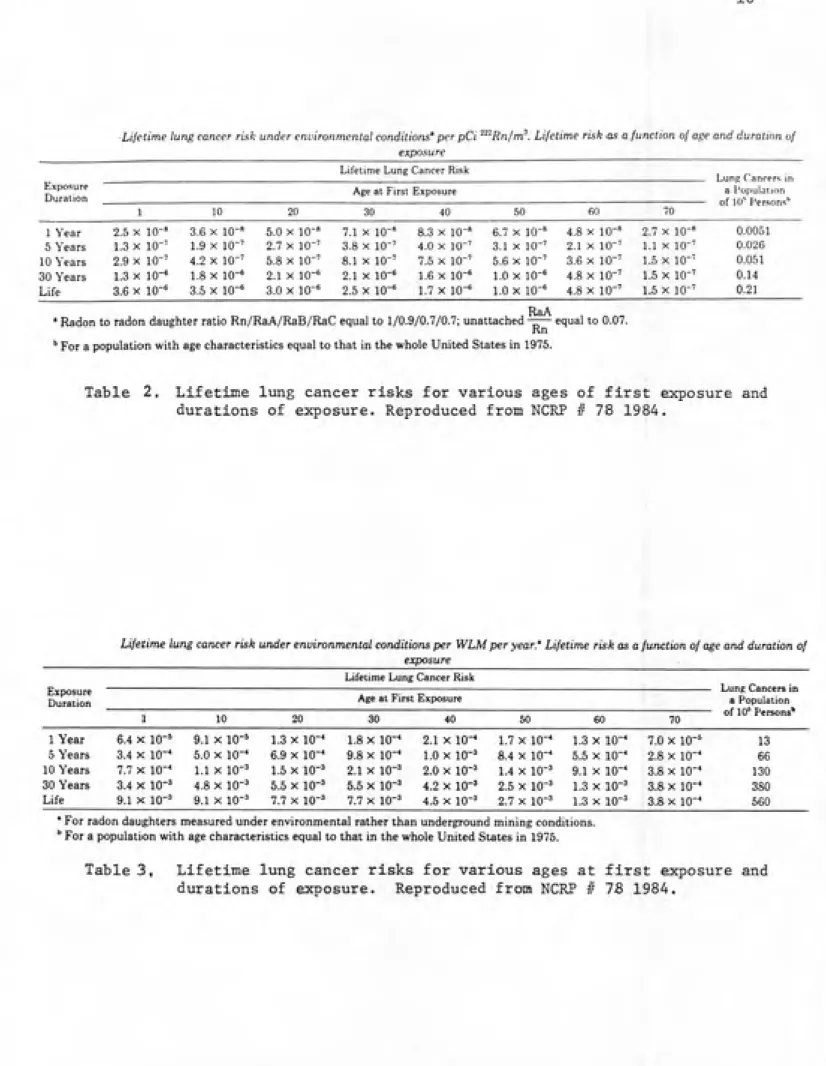
durations of exposure, see tables 2 and 3. The risks at the v lower radon daughter levels found under environmental conditions have been extrapolated down from the risks obtained from the higher radon daughter levels of the uranium miner data. The NCRP justifies this extrapolation by taking the conservative position that lung cancer induction is a stochastic or non-threshold type of response and therefore there is some risk even at the lower doses delivered by environmental levels of radon daughters.

Lifetime lung cancer risk under environmental conditions' per pCi ""^Rn/m^. Lifetime risk as a function of age and duration of

exposure

Lifetime Lung Cancer Risk Exposure

Duration

Age at FirstExposure a Population of 10' I'ersons''

1 10 20 30 40 50 GO 70

1 Year 2.5 X 10-" 3.6 X 10-» 5.0 X 10-' 7.1 X 10-» 8.3 X 10-« 6.7 X 10-' 4.8 X 10-' 2.7 X 10-" 0.0051 5 Years 1.3 X 10- 1.9 X lO"' 2.7 X 10-' 3.8 X 10-' 4.0 X 10"' 3.1 X 10-' 2.1 X 10-' 1.1 X 10-' 0.026 10 Years 2.9 X lO"' 4.2 X IQ-' 5.8 X 10-' 8.1 X 10"' 7.5 X 10-' 5.6 X 10-' 3.6 X 10-' 1.5 X 10-'

0.051 30 Years 1.3 X 10-« 1.8 X 10-« 2.1 X 10-^ 2.1 X 10-' 1.6 X 10-' 1.0 X 10-' 4.8 X 10-' 1.5 X 10-'

0.14

Life 3.6 X 10"^ 3.5 X 10"' 3.0 X 10-' 2.5 X 10-' 1.7 X 10-' 1.0 X 10"' 4.8 X 10-' 1.5 X 10"' 0.21

RaA

• Radon to radon daughter ratio Rn/RaA/RaB/RaC equal to 1/0.9/0.7/0.7; unattached —— equal to 0.07.Kn

'' For a population with age characteristics equal to that in the whole United States in 1975.

Table 2. Lifetime lung cancer risks for various ages of first exposure and

Lifetime lung cancer risk under environmental conditions per WLM per year.' Lifetime risk as a function of age and duration of

exposure

Lifetime Lung Cancer Risk

Lung Cancers in a Population of 10* Persons' Exposure

Duration Age at First Exposure

1 10 20 30 40 50 60 70

1 Year 6.4 X 10-' 9.1 X 10-' 1.3 X 10-* 1.8 X 10-* 2.1 X lO-* 1.7 X 10-* 1.3 X 10-* 7.0 X 10-' 13 5 Years 3.4 X IQ-" 5.0 X 10-' 6.9 X 10-* 9.8 X 10-* 1.0 X 10-' 8.4 X 10"* 5.5 X 10-* 2.8 X 10-* 66

10 Years 7.7 X 10-* 1.1 X 10-' 1.5 X 10-' 2.1 X 10-' 2.0 X 10-' 1.4 X 10-' 9.1 X 10-* 3.8 X 10-* 130

30 Years 3.4 X 10-' 4.8 X 10-' 5.5 X 10-' 5.5 X 10-' 4.2 X 10-' 2.5 X 10-' 1.3 X 10-' 3.8 X 10-* 380 Life 9.1 X 10-' 9.1 X 10-' 7.7 X 10-' 7.7 X 10-' 4.5 X 10-' 2.7 X 10-' 1.3 X 10-' 3.8 X 10-* 560

* For radon daughters measured under environmental rather than underground mining conditions.

*ͣ For a population with age characteristics equal to that in the whole United States in 1975.

Table 3, Lifetime lung cancer risks for various ages at first exposure and

durations of exposure. Reproduced from NCRP # 75 1984.

wuyi/yr)(9.1 x lOE --3 per WLM per year) = 1.8 x lOE -3 lung

cancers. This risk multiplied by the size of the U.S.

population would yield the number of excess lung cancers to

be expected in a lifetime due to exposure to average

environmental levels of radon daughters. The 0.2 WLM/yr

exposure can be expressed as continuous exposure to a radon

concentration of 0.8 pCi/L by the conversion shovm below

(assuming 50 percent eguilibrium of radon daughters).

0.2 WLM Yr 200 pCi/L „ „ _. ,^

---^--- -30lM---~WL~~ = °-^ P"^^^"^

By the same conversion process an exposure level of 1.0

WLM/yr corresponds to a concentration of 4 pCi/L which is

the indoor radon concentration at which remedial action is

recommended by the E.P.A., assuming 50% equilibrium of radon

daughters (EPA 1986).

The source of airborne radon is radium-226 decay in the

earth's crust (NCRP #45 1975, NCR? #77 1984, NCRP #78 1984).

The chemically inert gas emanates from porous rocks and

soils into the air above ground. Homes which are located on

top of soils with high emanation rates are effective at

trapping significant amounts of the emanating radon if their

ventilation rates are low. Relatively high indoor radon

concentrations (4 pCi/L or more) can be reduced roughly to

the outdoor concentration by a ventilation rate of about

four air changes per hour (NCRP #78 1984) . The average

outdoor radon concentration is often given as 0.2 pCi/L

high ventilation rate necessary to ensure low indoor radon

concentrations. As a result, houses in many areas of the

United States have high radon concentrations indoors. It is

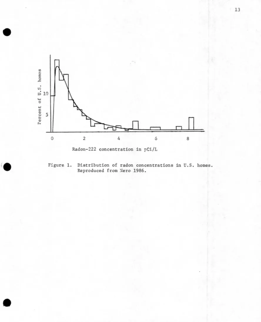
estimated that about two percent or 1.0 to 1.6 million of

the houses in the U.S. have indoor radon concentrations at

or above 8 pCi/L, see figure 1 (Nero 1986) . This is

equivalent to about 2.0 WLM/yr which is the exposure limit

recommended by the NCRP for an individual of the general

population (NCRP # 77 1984). The exposure limit for a

radiation worker is 4 WLM/yr (NCRP #77 1984).

Radon in groundwater

Although the greatest contribution to indoor radon is

from soil emanation, radon will also emanate from building

materials if significant amounts of uranium-238 decay

products are present and from the home's water supply if it

contains significant concentrations of radon. The latter

possibility is of concern in this groundwater sampling

project conducted in North Carolina.

A chemically unreactive gas is retained in water only

to the degree that it is soluble in water. Radon is

slightly soluble in water and can therefore be transported

by water. But it can also easily escape from the water into

the airspace above it if the water lies stagnant, or even

more so if the water is agitated or aerated. The water

supply to a house enters via a sealed system of plumbing

that prevents escape of radon, but at points of direct water

2 4 6 Radon-222 concentration in pCi/L

Figure 1. Distribution of radon concentrations in U.S. homes.

opportunity for the radon to be released into the home

environment. Bathroom, laundry and kitchen facilities are

major sites where radon from the water supply could enter

the home.

The questions of interest then become, how much radon

is present in a typical water supply and how much radon is

released indoors from a given level of radon in the water?

These are difficult questions to answer accurately and

require collecting a lot of data. It has been estimated

that a radon concentration of 10,000 pCi/L in a home's water

supply will contribute approximately 1 pCi/L radon indoors

(Duncan 1976). This relationship is an average and will

vary somewhat as characteristics vary from house to house in

terms of their ability to trap the emanating radon.

In addressing the question of radon concentrations in

water supplies the first consideration should be the source

of the water. Dwellings that draw on open bodies of water

such as lakes or rivers should not exhibit a high radon

concentration in their water because most of the gas will be

released through the large surface area available for

emanation before the water enters the home. Homes supplied

by large groundwater systems should also be less likely to

show high radon concentrations in the water entering them

because the size of the system usually results in long time

periods between extraction of the water from the ground, and

its use in individual homes. This time factor affords

daughters and emanation of radon from the water while stored

in tanks or towers. By contrast, in small groundwater

supplies water is used in homes much sooner after removal

from the ground. If the formations containing the

groundwater are rich in the parent nuclides of radon and if

the rock is porous enough radon can easily dissolve in the water and be transported to sites where the water is tapped

for human use.

Geological influence

The question regarding how much radon is in a

ground-water supply relates to the long range goal mentioned

earlier, the formulation of a predictive model of radon

concentration based on site characteristics and well parameters. In order to describe such a model different

factors that influence radon concentrations need to be identified.

One factor is the type of rock from which the

ground-water originates. Since radon is a link in the natural uranium decay series, water coming from rock formations rich

in uranium-238 or its decay products is likely to contain a

lot of radon. Previous studies have found significantly

elevated radon concentrations in North Carolina groundwater

supplies (Sasser and Watson 1978, Horton 1983) with one

third of the samples in the former study showing radon

concentations over 2000 pCi/L and several samples in the

range of tens of thousands of pCi/L. A review of radon

highest concentrations to be in the Appalachian-Piedmont

regions of the eastern states (Hess 1985) which includes a

large portion of North Carolina. The Appalachian-Piedmont

area is comprised of granite rock formations which are

characteristically high in uranium-2 38 from which radon is

formed.

Comparison of radon concentrations measured in North

Carolina (measured in previous studies) with site geology

showed radon concentration to be associated with rock type.

The highest concentrations were found in groundwater from

sites located in granite formations (geometric mean equals

5900 pCi/L, Loomis 1985). Gneiss, schist and metavolcanic

regions of North Carolina contained groundwater with lower

radon concentrations with a geometric mean of about 1200 to

1300 pCi/L and the rock types of the coastal plain area

showed the lowest radon concentrations in groundwater

sampled (Loomis 1985). The association between site geology

and radon concentration in groundwater is examined as one of

the two objectives of this report. A statistical test for

differences in measured radon concentrations between the

geological groups sampled in North Carolina is applied in

the data analysis section of this report.

Other factors besides geology could influence varia¬

tions in radon concentrations in groundwater. Among them

are the porosity of rock strata, the ratios of parent

nuclides of radon in the rock, the quantity of water present

ground and time or climatic variations. Some of these are

addressed in the report to the Water Resources Research

Institute (Loomis 1987) but are not given any more attention

here.

For this study it was decided that small public water

supplies would be used for sample collection. In North

Carolina these are systems serving 25 persons or more with

water from one to several wells located in the vicinity of

the user population. An advantage of sampling public water

supplies is that the state requires that public records be

kept for each well in such a supply. This meant that owner

contact information and information needed to locate

potential sampling sites was on file. These are important

items of information to have in conducting a statewide

sampling project of this size. Also available on file were

the driller's pumping tests. These were used to obtain

information about each well for calculation of hydrologic

parameters under consideration for the predictive model of

MATERIALS AND METHODS

Two hundred and nineteen wells were selected for poten¬

tial sampling. The goal was to actually sample 100 of them

for the final dataset (20 from 5 geological groups). All

sites were wells that serve as small public water supplies.

Although it was not a requirement that they were actually

being used at the time of sampling, this was usually the

case. Choosing from public well water supplies facilitated

gathering owner contact information, pumping capacity data

and geological information for each site from public

records.

Data on individual wells needed for contacting the

owner and locating the well were obtained by Dana Loomis

from the state's Division of Health Services Water Supply

Branch computer files. The owners were initially contacted

by mail describing the sampling project and soliciting

permission to collect a sample from their well. A copy of

the driller's well record was also obtained from the Ground

Water Section of the North Carolina Department of Natural

Resources and Community Development for each well selected.

These provided data on exact location, total depth, drilling

date and the driller's pumping test. Pump test data were

used to calculate values of hydrological parameters for each

well.

Each site was assigned to one of five generalized geo¬

logical categories or rock types. This was based on surface

Survey maps. The final dataset was comprised of wells

sampled from granite rocks, gneiss and schist rocks,

metavolcanic rocks, mafic rocks and the rocks of the coastal

plain region of North Carolina.

From the selected sites a sample of 100 was randomly

chosen (20 in each of the 5 rock groups) . Their locations

were marked on a state map to organize sampling trips that

would maximize collection efficiency. Owners of wells were

contacted by telephone to arrange specific meeting times for

sampling each well.

Two sample analysis techniques were used during this

work. The technique of radon emanation into a scintillation

cell was performed on all samples, and a liquid

scintillation counting procedure was performed concurrently

on about half of the sampled sites (Horton 1983). The

emanation process will be discussed first.

Emanation

Sample collection for analysis using the emanation

technique was made at a water faucet located as close to the

wellhead as possible. Every attempt was made to obtain

samples that were representative of fresh groundwater. This

meant avoiding water from pressure tanks, storage tanks,

water towers or outlets distant from the wellhead. In

addition the pump in the well was switched on and the

collection valve was opened to allow water to flow from the

well for several minutes before sample collection. To

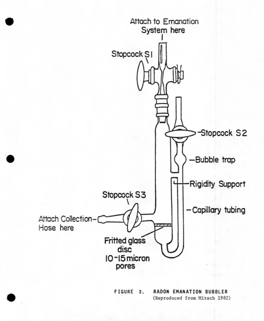
rubber hose was fitted to the faucet. The other end of the

hose was attached at the collection stopcock S3 of the

emanation bubbler shown in figure 2. Water was allowed to

enter the bubbler displacing the air through the open

stopcock at the top of the bubbler (stopcock SI). Stopcock

32 remained closed. If turbulence was evident the water was

discarded and the flow rate reduced further until a sample

was obtained without aeration. Since radon is a chemically

unreactive gas it may be lost rather easily from the sample

if there is much aeration of the water during collection.

When the bubbler was approximately three quarters full

collection was stopped by rapidly closing stopcocks S3 and

SI in that order. The bubbler was then disconnected,

labelled and carefully stored for transportation. Time and

date of collection were noted for each sample. One sample

for emanation analysis was taken at each site. Samples were

transported back to the Radiological Hygiene Laboratory for

analysis as soon as possible. Samples were emanated within

one to two days of the time of collection.

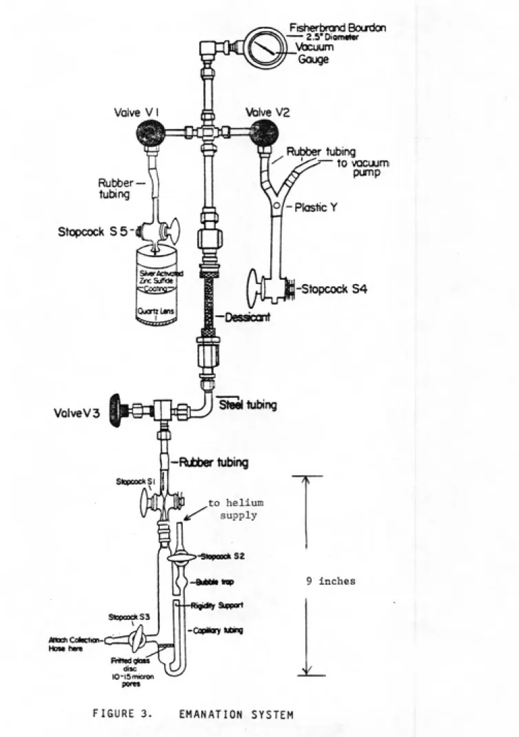
The emanation apparatus used for analysis is shown in

figure 3. It consists of stainless steel seamless tubing

(I.D. of 0.25 inches), clear plastic tubing and hose clamps

of various sizes, glass stopcocks, silicone sealant, Whitey

valves, Swagelok fittings, calcium sulfate desiccating

material and a Fisher vacuum gauge. Prior to use each day

the system was evacuated in order to assess its ability to

Attach to Emanation

System here

I

Stopcock S!

Attach

Collection-Hose here

^

Stopcock S3

-Stopcock S2

—Bubble trap

Rigidity Support

-Capillary tubing

Fritted glass

disc

10-15 micron

pores

FIGURE 2. RADON EMANATION BUBBLER

Vaive VI

Ftsherbfond Bordon — Z.S'Diomfrter

Vbcuum Gauge

VQlve V2

Rubber —

tubing

Stopcock

S5-Rubber tubing

ͣ

to vcscuum pLtfnp

Silver tetiwol Id ZncSulWe

VolveV3

Ojortzlans

o/-Plastic Y

^/v-u-fl

'Dessicant

StopcockSl

Steel tubing

-Rubber tubing

to helium supply

Attach Coiection-Hose twr«

RigicMy Support StopoocfcS3

-CapMry Uxng

RiltGdQloss

disc 10-15 micron

pores

Stopcock S4

9 inches

inches mercury over thirty minutes was judged as acceptable.

The scintillation cell to be used for the emanation of a

given sample was flushed and filled several times with

helium gas and counted for background for thirty minutes

just prior to the emanation. Helium was used during

background counting because helium was also used during the

emanation. The emanation was performed following the

procedure outlined in the technical report of Barry Mitsch

(Mitsch 1982). The sample bubbler and scintillation cell

(with all stopcocks closed) were attached to the emanation

system as shown in figure 3. The helium supply was then

attached, valves VI through V3 were opened, stopcock S4 was

closed and the system was evacuated by switching on a vacuum

pump attached as indicated in the figure. Stopcock S5 on

the scintillation cell was then opened and the drop in

vacuum was noted to be certain the cell was evacuated.

After 1 to 2 minutes the system was sealed off from the pump

by closing valve V2. The vacuum pump was returned to

atmospheric pressure by opening stopcock S4. The emanation

was initiated by very slightly opening stopcock Si at the

top of the bubbler. The difference in pressure draws gases

out of the water and into the system. Once the pressure

equalized the stopcock was opened fully. The bubbling was

maintained by slightly opening stopcock S2 on the bubbler to

allow pressurized helium to continually flow through the

bubbler and the system. The rate of helium flow was used to

During the emanation, radon and helium gas pass through

filter paper barriers and desiccating material where water

vapor and radon progeny attached to particulates become

trapped. Care must be taken not to let water rise up into

the system during emanation or the desiccant and filters are

rendered useless. After a thirty minute bubbling time the

process was stopped by closing stopcock S5 on the

scintillation cell sealing in any radon that was transferred

from the sample. Next, stopcocks SI and S2 were closed to

seal the water in the bubbler. The rest of the system was

returned to room pressure and the cell was disconnected and

stored in a light tight box to allow equilibration between

radon and radon progeny. A minimum equilibration time of

four hours was always used.

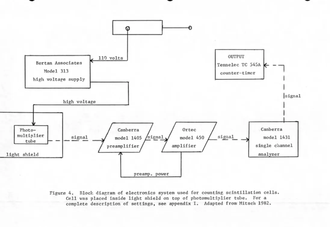
The electronic counting system used is depicted in fig¬

ure 4. The components used are indicated. For a complete

description of equipment settings used see appendix I.

Prior to any background or sample counting for the day and

at the end of counting the consistency of the system was

tested. A standard activity scintillation cell was used for

this testing. Ten one minute counts were recorded and

averaged. For background and sample counting, scintillation

cells were counted for thirty minutes. Since emanation was

performed for thirty minutes, a series of several samples

could be efficiently analyzed by simultaneously emanating

one sample into a scintillation cell while counting the

Model 313

high voltage supply

Photo-multiplier

tube

light shield

high voltage

signal

counter-timer

Canberra

model 1405 /^iSB^l

preamplifier

----71^----Ortec model 450

amplifier

signal

preamp. power

n

signal

Canberra model 1431

single channel analyzer_____

Figure 4. Block diagram of electronics system used for counting scintillation cells.

Cell V7as placed inside light shield on top of photomultiplier tube. For a

was counted once after a minimum four hour ingrowth.

Liquid scintillation

Sample collection for liquid scintilltion analysis was

made immediately after and at the same outlet where samples

were taken for emanation analysis. To collect the sample

the water flow rate was reduced, clear plastic tubing was

fitted to the outlet and a four inch diameter funnel was

attached to the free end of the tube. Holding the funnel

upright the water was allowed to pool and slowly overflow

the edges until all air pockets had been purged from the tubing and no turbulence was evident in the water. A 20 cc

syringe with 18 gauge needle was inserted one to two inches below the water surface. As the water continued to flow the

syringe was flushed a few times discarding the water each

time. The final 10 ml sample was drawn into the syringe and

immediately expelled at the bottom of a 20 ml glass liquid

scintillation counting vial already containing 10 mis of a mineral oil based scintillation fluid. Care was taken to

draw the water into and expel it from the syringe slowly to

minimize aeration of the sample. The dense water layer

remains at the bottom of the vial and the organic layer on

top helps prevent the escape of radon as the water is introduced into the vial. Two vials were filled at each

site and the time and date of collection were noted. Once

transported to the Radiological Hygiene Laboratory the vials

were counted within one to two days of the time of

Counting was done using a Packard Tri-Carb 300 liquid scintillation counter preprogrammed to count each vial for

50 minutes or until the percent deviation was down to 2

percent. The energy windows were set to count from 0 to

2000 KeV. Two background vials were counted with each batch

of samples. One background vial contained only 10 ml of

scintillation fluid and the other contained scintillation fluid plus 10 ml of distilled water. No standard activity

vials were counted with samples because none were available

when sampling for liquid scintillation counting began. Just

prior to starting counting, each vial was shaken for about

15 seconds to mix the two fluid phases. According to the

EPA protocol (Horton 1983) the radon in the water sample

preferentially dissolves in the organic scintillator layer

and any radium present remains dissolved in the aqueous

layer. The batches of vials were counted after four hours

in order to allow for equilibration of radon daughters. See

appendix II for step by step details of the liquid

scintillation counting procedure used.

Calibrations

In order to calculate sample radon concentrations from

count rate data collected by either analysis technique a

calibration factor was needed relating count rate to

activity present in the sample. This was obtained by

analyzing a sample of known activity in exactly the same way

that unknown samples were analyzed. The net count rate

observed was then divided by the known activity contained in

the standard. This factor (counts per minute per unit

activity) was then divided into the count rate from an

unknown sample to convert to sample activity.

Separate standard activity sources were needed for the

two analysis procedures. Two standard bubblers made

previously by a Radiological Hygiene student were initially

used for the emanation system (Carver 1980). By allowing

the source to remain sealed for approximately thirty days

the activity of radon equilibrates with that of the radium.

The bubbler is then processed as if it were a sample of

unknown activity. Calibration factors obtained from

analyses on the two standard bubblers were inconsistent with

values obtained in previous work by Barry Mitsch (Mitsch

1982).

Since the completion of sampling, two other sources of

radium have been obtained. The first was through

participation in an interlaboratory quality control program

with Lockheed Engineering and Management Services, Las

Vegas, Nevada. The program was designed to assess the

reliability of environmental radon measurement efforts by

laboratories across the country and to test the performance

of a new radium-226 source package they had fabricated. We

were provided with a bottle containing a known amount of

radium-226 activity dried on a piece of filter paper which

was sealed between two pieces of clear plastic. The sealed

source packet was immersed in the bottle full of water.

seal into the water while the radium does not (as long as

the water tight plastic seal remains intact). By allowing

the bottle to remain sealed for thirty days the radon

activity equilibrates with the radium activity. The

standard activity water was analyzed by carefully

transferring aliquots to bubblers and counting vials. The

procedure can be repeated by simply refilling the source

bottle and allowing for ingrowth again.

The second new radium source was obtained from the

Environmental Protection Agency in Las Vegas, Nevada in the form of an aqueous solution. From this solution dilutions

were made in two bubblers and five sealed liquid

scintillation counting vials. See appendix III for a step

DATA ANALYSIS

One hundred sampled wells are included in the final dataset. All wells were sampled for emanation analysis. Only fifty two were sampled for liquid scintillation analysis because sampling began before the liquid scintillation counting procedure had been set up. Samples

were collected from May through November 1986. The radon

concentration data obtained for the 100 sites are shown in

appendix IV. The data are sorted by five geological classifications of sites sampled. Radon concentrations in pCi/L were calculated from net count rates obtained from sample analyses. The relationship used is shown below.

Rn-222 cone. (pCi/L) = --1---^°°° "'^/^ ^^ ^^t)

where;

X = net count rate (cpm)

Y = calibration factor (cpm/pCi) V = sample volume (ml)

> = radiological decay constant for radon

(1.8 X lOE-1 daysE-1)

t = elapsed time from sample collection to midpoint

of count (days).

Calibration factors

As stated in the methods section, samples of known ac¬ tivity were analyzed to obtain calibration factors in counts

per minute per picocurie (cpm/pCi). Calibrations for the

31

emanation standards were inconsistent. One value (4.73 cpm/pCi) agreed well with previous results while the other did not (3.27 cpm/pCi) . It was concluded that these old

emanation standards were no longer reliable, and that an

average calibration factor from previous work (4.61 cpm/pCi)

should be assumed (Mitsch 1982) until the old standards

could be replaced.

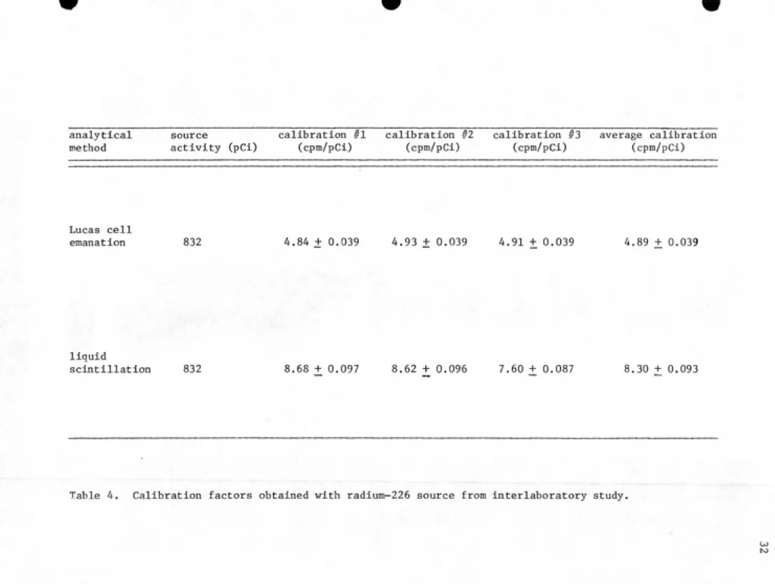
A new sealed radium-226 source from an interlaboratory

quality control study provided a convenient means of generating water containing a known radon activity. Aliquots of this water were dispensed into emanation bubblers and liquid scintillation counting vials and analyzed in the usual manner. Results of this work are shown in table 4. Results from other laboratories participating in the study are shown in table 5.

In addition, an aqueous radium-226 source obtained from

the Environmental Protection Agency in Las Vegas was diluted

into a stock solution which was used to make sealed standard

bubblers and vials. The procedure used for this is given in

detail in appendix III. Results from analyses of these new

standards are shown in table 6. The emanation calibration

Lucas cell

emanation 832 4.84 + 0.039 4.93 + 0.039 4.91 + 0.039 4.89 + 0.039

liquid

scintillation 832 8.68 + 0.097 8.62 + 0.096 7.60 + 0.087 8.30 + 0.093

Table 4. Calibration factors obtained with radium-226 source from interlaboratory study.

Emanation method

Laboratory Calibration factor

(cpm/pCi)

5 3.79 + 0.08

8 4.24 ± 0.04

14 2.50 ±. 0.04

16 4.78 + 0.13

*17 4.89 jL 0.04

19 4.67 Ji 0.21

21 4.66 + 0.15

24 4.57 ± 0.24

25 1.53 + 0.13

28 0.105

Liquid scintillation method

(cpm/pCi)

1 8.88 + 0.00

2 8.25 J^ 0.23

3 7.26 +. 0.19

4 8.45 Jl 0.05

6 8.13 J^ 0.34

7 7.50 +. 0.23

10 8.59 + 0.06

11 7.51 t 0.45

13 6.75 Ji 0.08

15 7.70 i 0.17

*17 8.30 Ji 0.49

18 8.40 +_ 0.08

18 8.12 ± 0.37

20 8.08 jL 0.10

21 8.19 i 0.05

21 9.12 jt 0.09

23 6.82 ± 0.003

26 9.00 ± 0.09

27 3.64

27 3.34 ± 0.47

* indicates Radiological Hygiene Lab

Table 5. Calibration factors obtained by participants in interlaboratory study. Adapted from personal communi¬ cation from E.L. Whittaker, Lockheed Engineering and Management Services Company, Environmental Programs Office, 1050 E. Flamingo Road, Suite 120, Las Vegas,

Lucas Cell Emanation

Activity (pCi) Calibration (cpm/pCi)

238 5.67 ± 0.032

476 5.38 ± 0.022

* 5.53 ± 0.027 (average)

Liquid Scintillation Counting

Activity (pCi) Calibration (cpm/pCi)

238 10.87 ± 0.11

476 10.96 JL 0.11

714 10.85 ± 0.11

952 10.78 ± 0.11

1190 10.84 ± 0.11

10.86 ± 0.11 (average)

Table 6. Calibration factors obtained with dilutions from

aqueous radium-226 source from the Environmental

Protection Agency in Las Vegas, Nevada.

* Analyses of the two standard activity emanation

bubblers has been repeated. The resulting calibrations were 5.61 cpm/pCi for the 238 pCi standard and 5.11 cpm/pCi for the 476 pCi standard. The overall average

for emanation and liquid scintillation counting were used

for final calculations of radon concentration. The

standards from which these data were obtained are sealed and

do not require handling of an aliquot prior to analysis.

The final average calibration factor used to calculate

the emanation radon concentrations (table 6) represents a

20% increase over the average value of 4.61 cpm/pCi

previously used (Mitsch 1982) . Although this is a

significant increase, it should be noted that quality

assurance emanation experiments performed at U.N.C. in

cooperation with the E.P.A. in Las Vegas produced

consistently high radon measurements (Mitsch 1982). It was

proposed that error in the calibration factor was the

greatest contributor to these high radon measurements (Hayes

1984). Consistently high radon measurements could be

explained by the calibration factor being too low (see

previous expression for calculating radon concentration).

The quality assurance radon measurements performed by Mitsch

were an average of 23 percent too high.

Exploratory data analysis

The data in appendix IV include radon concentrations

determined by both emanation and liquid scintillation

analysis for fifty two out of one hundred sites sampled. An

objective of this study was to determine whether the liquid

scintillation counting procedure produced results consistent

with those of the standard emanation method. An exploratory

12000

11000

10000

u p.

c

•H

g •H U

to

1-1

c

o

c

o CJ

c

o •o R)

Pi

9000

4000

3000

2000

1000

Emanation Liquid scintillation

Figure 5a. Box plots of radon concentrations as determined

cr

u

(U

Pi

itO.5 0.5 1.0 1.5 2.0 2.5 3.0 3.5 7.8 11.0 Radon-222 (10 pCi/L)

Emanation

a*

(-1

M-l

erf

I I [ IM .

«i::0.5 0.5 1.0 1.5 2.0 2.5 3.0 4.5 5.0 7.5

Radon-222 (10 pCi/L)

Liquid scintillation

indicate great differences in radon concentrations between

the two datasets. However, the histograms indicate that the

data for both analytical techniques are not normally

distributed. In addition, the box plots show that there are

outlying data points present. The box in the figure

represents the interquartile range (IQR) or the middle 50

percent of the data. The line across the box is the median

value (50th quartile) , the ends of the box represent the

25th and 75th quartiles. The length of each stem represents

up to 1.5 times the IQR, depending on where values fall in

this area. Shorter stems result when data points are

lacking in the stem region. Values extending beyond the

stems are called outlying data points. Outliers may be

present regardless of the length of the stem. The nonnormal

distribution of the data violates an assumption of the

classical statistical test employed in this section to

compare the two analysis techniques. This indicates that a

transformation of the data or other robust method of

statistical analysis will be needed. The hypothesis testing

section will describe this in greater detail.

Figure 6 shows a scatter plot of radon concentrations

measured in the groundwater of the fifty two sites analyzed

by both emanation and liquid scintillation counting methods.

If the two analysis procedures produce similar results for

the same sites sampled, then the slope of the best fit line

through the data in the scatter plot should be equal to one.

100000

y 10000

5

100 1000 10000 100000

Radon-222 concentration by emanation (pCi/L)

Figure 6. Radon concentrations as determined by emanation versus liquid scintillation analysis. Slope of the line

through the data is equal to one.

(dependent variable) on the emanation data (independent

variable) yields a slope of 0.94 indicating that on the

average the emanation results are slightly higher. A

Pearson correlation matrix for the two variables generated a

correlation coefficient of 0.98, which is highly

significant.

The other primary objective of this study was to de¬

termine whether there were significant differences in radon

concentrations in groundwater sampled from different

geological formations. Figures 7a and 7b show the radon

data grouped in five geological classifications for

emanation and liquid scintillation counting analysis

respectively. Examination of the grouped data shows

nonnormal distributions (note off center locations of

medians), outlying data and inequality of variance between

groups (note different length boxes). Again, because the

data do not satisfy test assumptions well, robust methods

will be used in the next section to test the influence of

geology on radon concentration.

Hypothesis testing 1

Hypothesis tests are used to answer experimental ques¬

tions on a statistical or probabilistic basis, and to make

inferences about a population based on a sample from the

population. Each question is expressed in the form of two

hypotheses concerning a population parameter selected to

represent the population. The hypothesis tests establish a

30000

20000

13000

o 6000

Cfl

C

Cfl

B

<U

^ 5000

c

o •H

4-1

^ 4000

o

n

o o

^ 3000

I

o Xi

cfl

2000

1000

X CP n=20

GN GR ͣMA

n=23 n=18

Rock types

n=17

MV n=22

Figure 7a. Box plots of radon concentrations, grouped by rock type,

as determined by emanation analysis. Rock types: CP=coastal

20000. 13000-a g

^

.1 5000

•^ 4000

Figure 7b. Box plots of radon concentrations, grouped by rock type, as determined by liquid scintillation analysis. Rock types: CP=coastal plain, GN=gneiss & schist, GR=granite, MA=mafic,

produce a test statistic calculated from parameters of the

sample. The test statistic is compared to a tabulated

critical test statistic of a specified confidence level,

which assumes the null hypothesis. The decision to accept

or reject the null hypothesis is made based on whether the

sample statistic exceeds the critical value. Before a test

can be performed, certain prior conditions must be satisfied

as nearly as possible. Checking to see if these conditions

were met was the purpose of the exploratory analysis, which

revealed that certain assumptions were not well satisfied.

The question which asks whether liquid scintillation

analysis produced results comparable to standard emanation

analysis is tested by looking at the differences between the

two measurements for each site sampled. A one sample paired

T-test is used because the samples were collected at each

site in pairs (Koopmans 1987). The null hypothesis states

that the mean difference (in the population) equals zero,

meaning the two techniques yield the same results. The

alternative states that the mean difference does not equal

zero. The test statistic is calculated using sample

estimators of the population parameters. Exploratory

analysis of the fifty two pairs of emanation and liquid

scintillation data in figures 5a and 5b indicated the need

for a modified hypothesis testing method. Figure 8 shows a

box plot of the differences in radon concentrations measured

by the two analytical techniques. The outlying data points

1600

1400

1200'^

1000'

800

u

600

p.

o •H

4J

CD 400 M

4->

200

g

u

0

CM

c

o

•d

ct) _-200 C

•H

(0 _-400

U

C!

<U Vj 0)

4-1 -600

«M

•rl

P

-800

-1000

-1200

-1400

-1600

Figure 8. Box plot of the differences in radon concentrations

measured by emanation versus liquid scintillation

analysis. Differences were calculated by subtracting the

of the differences and therefore can reduce the power of the

T-test. Trimming outliers from the dataset before

performing the test restores much of the power (Koopmans

1987). The outliers are trimmed so that the data better fit

the conditions of the hypothesis test used. The term

outlier is being used to describe data points which deviate

from the mean to a much greater degree than most of the

data. It is not implied that outliers are data which are

suspected of being the result of improper experimental

analyses. The T-statistic calculated from the trimmed data

is shown below.

T=

^T

T= 2.954

where: Xj= 10% trimmed mean difference =79.6 pCi/L

Sy= trimmed standard deviation = 170.5 pCi/L

Np= trimmed sample size =40

The critical value at the 95 percent confidence level for

this test is 2.042. Since the sample statistic exceeds

this, the null hypothesis is rejected with 95 percent

confidence. Therefore it is inferred, based on the sample,

that there is a significant difference in radon

concentrations measured by the two techniques.

Figure 9 shows a box plot of the differences expressed

0) o

c

Q)

Q)

14-1 14-1 4J

C

o

0)

P-i

100,

90

80

70

60

50

40

30

20

10

Figure 9. Box plot of percent differences in radon concentrations

measured bj' emanation versus liquid scintillation analysis.

examination of the percent differences in appendix IV and

their distribution in figure 9 shows that only five values

are greater than 45 percent difference. Alternatively,

forty five of fifty two values are below 35 percent difference and forty values are below 25 percent difference. Although there are statistically significant differences between emanation and liquid scintillation results, the

majority of them can be considered relatively small on a

practical basis.

With modification of sampling materials and procedures

used, these differences could be substantially reduced.

Noting the signs of percent difference values in appendix

IV, in 75 percent of the cases it is positive, indicating

that the emanation result is greater than the liquid scintillation result. The sample collection technique for

liquid scintillation analysis could provide insight as to

why these results were often lower. During collection a

water sample is drawn from a gently flowing, nonaerating

pool of water using a syringe. Careful attention must be paid to this procedure. The degree of success achieved in

executing this step with minimal radon loss may partially

account for the lower liquid scintillation results. By

comparison, samples for emanation analysis were collected

directly from a faucet, via rubber tubing, into the bubbler.

The potential for loss of radon during this collection

process is lower. The vials into which liquid scintillation

as well. Glass vials and plastic caps with paperbacked foil

liners were used in this study. Vial caps with better

sealing capabilities would reduce the likelihood of radon

loss due to leakage. It is also important to keep in mind

that the emanation result for each site is based on only one

sample while each liquid scintillation result is the average

of two measurements. Although it would require a

significant amount of extra time for analysis, it would be

best to obtain an average emanation result for each site.

By taking the following measures, substantial reductions in

the differences in radon concentrations measured may be

possible. Strict attention must continue to be given to

liquid scintillation sampling technique. To further reduce

the potential for radon loss after sampling, improved

collection vials should be used. Finally, an average result

for both analytical techniques should be obtained for each

site.

The other objective of the study, which asks whether

site geology has an influence on radon concentration, is

tested by looking at the variation in concentrations between

the five geological groups sampled. This is accomplished

using one way analysis of variance (Koopmans 1987). The

null hypothesis states that there is no difference in mean

radon concentration between any of the five groups. The

alternative is that there is a difference between at least

two of the groups. Exploratory analysis of the data in

the data prior to testing. In this case, the data are

transformed by taking their natural logarithms. Figures 10a

and 10b show the effect of the transformation on the data.

The data fit the test assumptions better, however outlying

data points persist in a number of the groups. Applying the

trimming technique to each group of the emanation data

improves the power of the test further. The analysis of

variance tables in table 7 show significant differences

between groups for both the emanation and liquid

scintillation counting data (the null hypothesis is rejected

in both cases). The liquid scintillation counting data were

not trimmed following the transformation because of the lack

of enough data in each group (see figure 7b for group sample

sizes) . The small sample sizes in some of the groups as

well as the variation in sample size between groups of the

liquid scintillation data has undoubtedly affected the power

of the analysis of variance test.

The analysis of variance indicates that for both eman¬

ation and liquid scintillation analysis at least two groups

have different mean radon concentrations. In order to tell

which groups are different, each mean is compared to the

other four individually by a least significant difference

method (Koopmans 1987). Results of these individual

comparisons are depicted in figure 11. The rock groups are

arranged in order of increasing mean radon concentration.

Groups that are inside sets of brackets were not

g ͣ H U CO e c O •H •U CO M 4-1 d u c o o c o 13 0) (-1 M-H o 00 o u 3 4J Cfl a 9 • 8 4 3 . 2 i

CP GN GR MA MV n=20 n=23 n=18 n=17 n=22

GN GR MA

n=23 n=18

Rock types

n=17

Figure 10a. Box plots of natural logarithms of radon concentrations, grouped by rock type, as determined by emanation analysis. Rock types: CP=coastal plain, GN=gneiss & schist, GR=granite,

u> Ui >^ H-CW C f-i (B 3

O pj 00 II o

fti 3 H M (jO <-a

II P) O O (W M c cr i-i ^ -a . P3 tn fO

3 H- Cl-H- CO bd

rt • o- o

(t) ^ M

^ 1^ H -a

ͨ

^ o

> n

O M O O

tt '^ !C rtCO 3II

B

P3 rt rt M

Hl^ͣv<! o M

H- ^ >xi t-u O (D (D

» CD - 3 pel

o

^ O S ?

R-II ^tJ »-<

S II n- p) rt

n> o n> H" Vl

n- o rt ͨo

P) pi n> M to

< en a o en

O rt a 0^

M P) p. pi

O M 3 i-i 3

PJ (D H- II o

3 13 a. rt a^ td

H- M O P) cr g

• t;-ͣ^ en

0

V

of r

liqu

II H- P3 OP p, p^

3 O ro cn 3

H- n 3

CD CD

^1

rt 3

II H 4>

g

(^ H- n

CD M 3

n B) rt

3* rt H H- H- P3

CD O rt

rt 3

H-B

en

3

II

sum of squares degrees freedom

between groups

within groups

64.1

70.2 71

16

0.99

16,211 0.001

(reject null hypothesis)

Dependent variable; In liquid scintillation result

sum of squares degrees freedom mean square

between groups

within groups

20.4

44.5 47

5.1

0.95

F-statistic p-value

5.385 0.001 (reject ntill hypothesis)

•

1

MA GR GN

Low radon-222 High radon-222

[

[

MV MA

GR GN

]

]

These two groups were not significantly different,

These two groups were not significantly different.

CP MV

Liquid scintillation

MA GR GN

Low radon-222

[

[

[

CP MV

MV MA

MA GR

]

]

High radon-222

These two groups were not significantly different.

These two groups were not significantly different.

GN These thr —' different

three groups were not significantly

Figure 11. Results of least significant difference groupings for emanation and liquid scintillation analysis. Rock groups are arranged by increasing mean radon concentration. Sets of brackets are intended only to depict which rock groups were not significantly different. Therefore, other combinations

significantly different.

Liquid scintillation precision

Two samples were collected at each site for liquid

scintillation analysis. This provides the opportunity for

testing the precision of liquid scintillation analysis by

applying a paired difference T-test to the data. The

results of the two measurements for each site are listed in

table 8. A one-sample paired T-test was performed on the differences between the two measurements obtained for each

site. The null hypothesis tested states that the mean

difference equals zero. The difference data are shown in

figure 12. The figure shows that the data contain outliers,

so it was first trimmed before applying the test. The

T-statistic calculated from the trimmed data is shown below.

^T

T = 0.914

where: X_= 5% trimmed mean difference =8.7 pCi/L S = trimmed standard deviation = 64.7 pCi/L

Nj= 46

The critical T-value at the 95 percent confidence level is

2.021. Since the sample statistic is less than 2.021, the

null hypothesis is accepted with 95 percent confidence.

Therefore it is inferred, based on the sample, that there is

no significant difference in radon concentrations measured

L.S. sample 1 L.S. sample 2 Pent diff (pCi/L) (pCi/L)

342 ± 17.7 370 + 17.7 7.7 675 + 19.5 651 + 19.4 3.6 292 i 16.5 331 ±. 16.7 12.5 254 ± 18.2 152 Jl 17.3 50.6 325 ± 18.2 539 Jl 19.7 49.4 691 i 18.5 709 Jl 18.8 2.6 2002 ± 27.7 1816 ± 26.0 9.8 1593 ± 25.1 1498 Jl 24.5 6.1 1958 + 27.5 2327 Jl 30.8 17.2 1113 ±. 23.0 1185 Jl 23.2 6.3 1297 ± 24.1 1241 _+ 23.8 4.5 2842 Jl 35.9 2832 i 35.8 0.4 1698 ± 26.2 1659 ±. 26.0 2.3 891 Jl. 22.1 926 JL 22.4 3.8 1362 ± 28.8 1397 J^ 29.0 2.6 288 ± 22.7 340 ^ 23.0 16.7 1215 Jl 21.8 1245 ± 22.0 2.5 7949 ±. 85.0 7644 Jl 82.0 3.9 2241 + 29.2 2121 ± 28.1 5.5

2065 ± 27.6 2086 Jl 27.8 1.0 1264 Jl 22.6 1170 + 22.1 7.7 484 i 18.3 516 +_ 18.6 6.4 3432 ± 40.8 3330 ± 39.8 3.0 284 + 17.2 311 + 17.4 9.0 1238 J: 22.9 1276 + 23.0 3.1 1114 Jl 22.3 1083 + 22.1 2.8 1018 Ji 21.9 1024 ± 21.9 0.6 1063 +. 22.2 1103 ± 22.5 3.7 359 i 19.4 323 Jl 19.2 10.4 175 J: 18.3 186 + 18.4 5.7 4949 ± 56.4 4834 d^ 55.3 2.4 3193 ± 39.4 3119 ± 38.7 2.3 1532 ± 22.4 1460 Jl 22.1 4.8 452 ± 16.7 497 Jl 17.1 9.6 9879 ±103.7 9942 J:104.4 0.6 2013 i 28.1 1975 + 27.8 1.9 1553 i 25.7 1439 + 25.0 7.7 238 ± 18.2 234 ± 18.2 1.7 2693 + 34.3 2762 + 35.1 2.5 4298 + 49.8 _{4524 ±} 52.0 5.1 2648 Ji 34.1 2620 ± 33.7 1.1 285 ± 15.4 267 ± 15.3 6.7 49 Jl 23.6 52 Jl 23.6 5.5 62 J: 23.8 94 ± 24.0 40.6 842 ± 28.9 857 + 29.0 1.8 104 ± 15.1 91 ± 14.9 13.1 3165 + 49.9 3073 ± 49.4 3.0 1967 ± 44.4 1948 + 44.2 1.0 1125 + 26.3 1090 ± 26.0 3.2 417 + 19.2 484 i 19.7 14.9 722 + 20.5 690 ± 20.3 4.6 1419 + 24.8 1486 + 25.2 4.6

Table 8. Radon concentrations determined by liquid scin¬

tillation analyses of two sample vials collected at 52

Figure 13 shows a box plot of the differences expressed

as percents. It should be noted that only three of the

values are above 40 percent difference, while forty nine of

the fifty two values are below 20 percent difference and

forty three values are below 10 percent difference. These

results show good reproducibility in the paired liquid

scintillation measurements. This is valuable information to

have since it lends credibility to the measurement

technique. The relatively few cases of larger percent

differences may be partially attributable to leakage of

radon from one vial of some of the pairs. Looking at table

8, it seems that the greatest percent differences are

associated with lower radon concentrations, indicating that

the difference expressed as a percent is large because the

concentration is low. However, this is not strictly the

case. A number of sample pairs at low concentrations have

low percent differences between them. Figure 14 shows a

plot of the differences between radon concentrations

measured in dual LSC samples versus the mean of dual LSC

samples.

In general, the results of hypothesis tests should be

taken with some reservation. Factors which can affect test

validity and power should be considered. This is

particularly true when considering the effect of a variable,

such as geology, on measured radon concentrations. Since

inferences are made about the population based on small

(pCi/L)

-400 -300 -200

________k—

-100 100 200 300 400

Figure 12. Box plot of the differences between radon concentrations

measured in dual liquid scintillation samples.

Percent difference

0 10 20 30 40 50 60 70 80 90 100

p.

CO 0)

400 ,

300 ͣ

CO

G

•H

CM

CM

C-J

I

C

O

(0 u

200.

CO

(J

C

(U !-i 0)

•H

Q

100,

-..N'

mean radon-222 concentration (10 pCi/L)

10

Figure 14. Plot of differences in radon concentration measured in