THE WAVE EQUATION ON SIMPLICES
By
Ziqing Lu
Senior Thesis
Department of Mathematics
University of North Carolina at Chapel Hill
March, 2019
ASYMPTOTIC BOUNDARY OBSERVABILITY FOR THE WAVE EQUATION ON SIMPLICES
ZIQING LU
Abstract. In this paper, we consider the wave equation on an n-dimensional sim-plex with Dirichlet boundary conditions. Our main result is an asymptotic observ-ability identity from any one face of the simplex.
1. Introduction
In this paper, we study the wave equation (∂t2 −∆)u = 0 on all n-dimensional simplex with Dirichlet boundary conditions. We obtain an asymptotic observability property from any one face of the simplex. This generalizes the result in [CS18] from triangles to to simplices inRn. The proof is similar to that of [CS18]. It uses
commu-tators and integration by parts arguments, but involves a coordinate transformation and linear algebra as well.
The formal statement of the problem is represented by (1.1):
(∂t2−∆)u= 0 on (0,∞)×Ω, u
∂Ω = 0,
u(0, x1, x2, . . . , xn) =u0(x1, x2, . . . , xn),
ut(0, x1, x2, . . . , xn) =u1(x1, x2, . . . , xn)
(1.1)
whereu is real-valued and u0 ∈H01(Ω)∩H3(Ω) and u1 ∈H01(Ω)∩H2(Ω). Regarding
this problem, the main theorem is the following:
Theorem 1.1. Let Ω ⊆ Rn be a simplex with faces F
0, F1, F2, . . . , Fn and suppose
u solves the wave equation on Ω. For any finite time T > 0, following we obtain the asymptotic observability identity for any one face of the simplex Ω:
Z T
0
Z
F0
|∂νu|2dS0dt=
T Area(F0)
nV ol(Ω) E(0)˜
1 +O
1 T
, (1.2)
where∂νu is the normal derivative onF0anddS0 is the induced surface measure. E(t)˜
is the conserved energy of the solutionu to the wave equation, defined by:
˜ E(t) =
Z
Ω
|∂tu|2+|∇u|2dV. (1.3)
Remark 1. Observability in this paper means we can observe the initial energy by taking a measurement on one face.
2. History
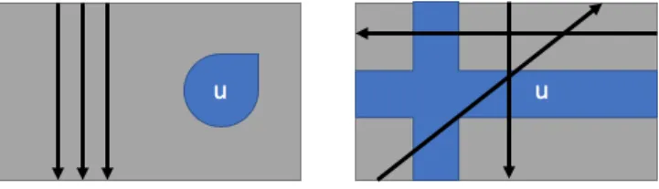
The study of observability is based on the prerequisite that waves propagate along straight-line paths in a homogeneous medium. Waves reflect off the boundary satisfying the law of reflection, so that the angle of incidence is the same as the reflection angle. The idea of observability originates from Rauch-Taylor’s paper [RT74] , where they studied geometric control for the damped wave equationutt−∆u+a(x)∂tu= 0. The idea is if every ray passes through the damping region wherea >0, energy decays exponentially as E(t) 6 Ce−t/c. For example, the first picture of Figure 1 is not geometric control while the second one is.
Figure 1. Rays Passing Through Subset Of Domain
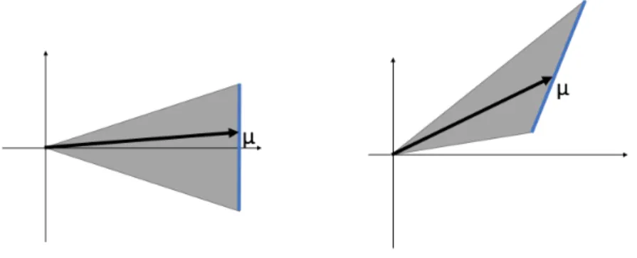
The closely related idea of observability asks if you can ”see” the initial energy by taking the measurement of a subset of the domain or a subset of the boundary. In the work of Bardos-Lebeau-Rauch [BLR92], the observability from a subset of the boundary was studied in depth. The condition for observability, similar to in Rauch-Taylor is that all rays hit the control region on the boundary transversally, as indicated inFigure 2.
Figure 2. Rays Hitting The Control Region On The Boundary
interested side. The result was obtained with an argument of the method of this paper, by the use of commutator and integration by parts arguments.
Figure 3. Asymptotic Observability On One Side Of Triangles
3. Preliminaries
This section of preliminaries provides lemmas and definitions required in the main proof.
Lemma 3.1 (Conserved Energy). For the solution u to the wave equation (1.1). The energy is conserved:
˜
E(t) = ˜E(0). (3.1)
Proof. Start with the wave equation (∂2
t −∆)u = 0. By multiplying ut and by inte-grating the wave equation on the domain, we have the following computations:
Z
Ω
(∂t2−∆)uutdV = 0
⇒ Z
Ω
∂t2uutdV −
Z
Ω
∆uutdV = 0
⇒ Z
Ω
∂t2uutdV +
Z
Ω
∇Tu∇utdV − Z
∂Ω
∂νuutdS= 0,
(3.2)
whereν is the outward unit normal vector and dS is the induced surface measure. Because u vanishes on the boundary, ut
∂Ω = 0 holds. We could therefore cancel
out the last term in the previous computation and prove that the energy is conserved due to result of (3.2):
˜ E0(t) =
Z
Ω
uttut+ututt+∇Tut∇u+∇Tu∇utdV
= 2
Z
Ω
uttut+∇Tu∇utdV
= 0.
(3.3)
Definition 3.1 (Elliptic Operator). A constant coefficient elliptic operatorP on Ω⊆ Rn is defined by
P =−
n
X
i,j=0
Kij∂xi∂xj, (3.4)
whereK is ann×nsymmetric, positive definite matrix.
Lemma 3.2(Ellipticity). Let Ω⊆Rnbe a simplex. Ifu∈H1
0(Ω)∩H3(Ω), then there
exists an constant C such that
k∇ukL2(Ω)6ChP u, uiL2. (3.5)
The following lemma is a modified version of Theorem 4 published in the paper [Chr17] by Christianson. The modified version can be directly used in the main proof of this paper.
Lemma 3.3 (Green’s formula for (3.4)). Let Ω0 ∈ Rn be the standard simplex and g
∂Ω0 = 0. LetP be an elliptic operator. Then for functionsf, g∈C
∞(Ω), we have,
Z
Ω0
(P f)gdV =
Z
Ω0
f(P g)dV +
Z
∂Ω0
f(νTK)∂gdSdt (3.6)
whereν is the outward unit vector on every face of the simplex Ω.
This paper inherits the notation that Christianson used in the paper [Chr17] to define higher dimension simplicies.
Definition 3.2 (Simplex). Let independent vectorsp~1, ~p2, . . . , ~pn∈Rn span from the
origin, then a simplex Ω in Rn is defined as:
Ω ={
n
X
i=1
cipi~ : n
X
i=0
ci 61 and ci >0, ~pi ∈Rn} (3.7)
We denote the face where ci = 0, i= 1, . . . , n as Fi and the remaining face F01.
Let matrix A be
| | |
~
p1 p~2 . . . pn~
| | |
. Because the column vectors p~1, ~p2, . . . , ~pn are
linearly independent, there exists an inverse matrix of A. Denote this inverse matrix by B.
In particular, we have standard simplex Ω0 ∈Rn.
Definition 3.3 (Standard Simplex). Let unit vectors e~1= [1,0,0, . . . ,0]T,
~
e2 = [0,1,0, . . . ,0]T, . . . , ~en = [0,0,0, . . . ,1]T ∈ Rn be n linear independent vectors.
The standard simplex, denoted by Ω0, is defined by all convex combinations of these linearly independent unit vectors:
Ω0={
n
X
i=1
diei~ : n
X
i=0
di 61 and di>0, ~ei∈Rn} (3.8)
This standard simplex has n+ 1 faces F00, F10, . . . , Fn0, where Fi0 is the face with di= 0, i= 1,2, . . . , n while the remaining face is F00.
The standard rectangular coordinates of the standard simplex Ω0 are denoted as (y1, y2, . . . , yn) in Rn while the rectangular coordinates of the original simplex Ω are
denoted as (x1, x2, . . . , xn) in this paper.
The following transformation takes the arbitrary simplex Ω inRnto the standard
simplex Ω0. Let ~x = [x1, x2, . . . , xn]T denote one vector in the simplex Ω and ~y = [y1, y2, . . . , yn]T denote the corresponding vector of~x in the standard simplex Ω0, then
we could obtain the following equation by considering the relation between the sets of basis of the simplex Ω and that of the standard simplex Ω0:
~
x=A~y (3.9)
For example, when ~y=ej~ = [0, . . . ,1,0, . . . ,0]T, where 1 is at thejth position of the vector, we have this relation:
~ x=
| | |
~
p1 p~2 ... p~n
| | |
ej~ =pj~ (3.10)
By observing this relation, we claim that ∇x = BT∇y after the transformation. The proof of this claim is inAppendix A.
Since the Laplacian operator is−∆x=−∇Tx∇xon the simplex Ω, the above claim implies this equation is equivalent to P =−(BT∇y)T(BT∇y) =−∇T
yBBT∇y on the standard simplex Ω0. Denote it byP.
According to (1.3), the energy of the solution to the wave equation iny-coordinate can be defined as :
E(t) =
Z
Ω0
|ut|2+|BT∇u|2dV. (3.11)
We claim that this energy is also conserved:
E(t) =E(0). (3.12)
Proof of (3.12).
E(t)0 =
Z
Ω0
uttut+ututt+ (BT∇ut)(BT∇u) + (BT∇u)(BT∇ut)
= 2
Z
Ω0
uttut+ (BT∇u)(BT∇ut)
= 0.
(3.13)
The method used in this proof is similar to that of Lemma 3.1.
Lemma 3.4. Consider the vector fieldX =Pn
i=0xi∂xi and the second order constant
coefficient symmetric operatorT =−Pn
i,j=1aij∂xi∂xj. Then:
Proof. Wheni=j,i= 1, . . . , n,
[−aii∂x2i, x1∂x1 +x2∂x2 +· · ·+xn∂xn]
= n
X
k=1
[−aii∂x2i, xk∂xk]
= [−aii∂2xi, xi∂xi] +
n
X
k=1,k6=i
[−aii∂x2i, xk∂xk]
=−aii∂x2i(xi∂xi) +xi∂xi(aii∂ 2
xi) +
n
X
k=1,k6=i
(−aii∂x2i(xk∂xk) +xk∂xk(aii∂ 2
xi))
=−aii∂xi(∂xi+xi∂ 2
xi) +xiaii∂ 3
xi+ 0
=−aii∂x2i−aii∂ 2
xi−xiaii∂ 3
xi+xiaii∂ 3
xi
=−2aii∂x2i
(3.15)
When i6=j,i, j= 1, . . . , n,
[−aij∂xi∂xj, x1∂x1 +x2∂x2 +· · ·+xn∂xn]
= n
X
k=1
[−aij∂xi∂xj, xk∂xk] +
n
X
k=1,k6=i,j
[−aij∂xi∂xj, xk∂xk]
= [−aij∂xi∂xj, xi∂xi] + [−aij∂xi∂xj, xj∂xj] + 0
=−aij∂xi∂xj(xi∂xi) +xi∂xi(aij∂xi∂xj)
−aij∂xi∂xj(xj∂xj) +xj∂xj(aij∂xi∂xj)
=−aij∂xj(∂xi+xi∂ 2
xi) +xiaij∂ 2
xi∂xj
−aij∂xi(∂xj+xj∂ 2
xj) +xjaij∂ 2
xj∂xi
=−2aij∂xj∂xi
(3.16)
4. Proof of the Theorem
Let the vector field be Y =y1∂y1 +y2∂y2 +· · ·+yn∂yn on the standard simplex
Ω0. ForP =−∇TBBT∇, we will compute:
Z T
0
Z
Ω0
[∂2t +P, Y]uudV, (4.1)
in two different ways. The two approaches are based on different ways of dealing with the commutator. One approach starts with using Lemma 3.4 while in the other approach we evaluate the commutator explicitly.
integration by parts gives:
Z T
0
Z
Ω0
[∂t2+P, Y]uudV dt=
Z T
0
Z
Ω0
2P uudV dt
=
Z T
0
Z
Ω0
(P−∂t2)uudV dt
=
Z T
0
Z
Ω0
−∇TBBT∇uudV dt− Z T
0
Z
Ω0
∂t2uudV dt
=
Z T
0
Z
Ω0
−(BT∇)TBT∇uudV dt− Z T
0
Z
Ω0
∂t2uudV dt
=
Z T
0
Z
Ω0
(BT∇)u(BT∇)udV dt+
Z T
0
Z
Ω0
∂tu∂tudV dt
− Z
Ω0
∂tuudV
T
0
=
Z T
0
Z
Ω0
|BT∇u|2dV dt+
Z T
0
Z
Ω0
|∂tu|2dV dt
− Z
Ω0
∂tuudV
T
0
=
Z T
0
Z
Ω0
|BT∇u|2+|∂tu|2dV dt−
Z
Ω0
∂tuudV
T
0
=T E(0)− Z
Ω0
∂tuudV
T
0
(4.2)
Notice that at the last step of the previous computation, we used result of (3.12) . We next compute (4.1) by a different approach. We first evaluate the commuta-tor explicitly and then use integration by parts. The second term generated by the commutator cancels out because of the homogeneous wave equation. Indeed,
Z T
0
Z
Ω0
[∂t2+P, Y]uudV dt=
Z T
0
Z
Ω0
(∂t2+P)Y uu−Y(∂t2+P)uudV dt
=
Z T
0
Z
Ω0
∂t2Y uu+P Y uudV dt
After we apply Lemma 3.3 to the second term and use integration by parts twice on the first term, we have:
Z T
0
Z
Ω0
∂t2Y uu+P Y uudV dt
=
Z T
0
Z
Ω0
Y u∂t2udV dt+
Z
Ω0
∂tY uudV
T 0 − Z Ω0
Y u∂tudV
T 0 + Z T 0 Z Ω0
Y uP udV dt+
Z T
0
Z
∂Ω0
Y u(νTBBT)∇udSdt
=
Z T
0
Z
Ω0
Y u(∂t2+P)udV dt+
Z
Ω0
∂tY uudV
T 0 − Z Ω0 Y u∂tudV T 0 + Z T 0 Z
∂Ω0
Y u(νTBBT)∇udSdt
= Z Ω0 ∂tY uudV T 0 − Z Ω0 Y u∂tudV T 0 + Z T 0 Z
∂Ω0
Y u(νTBBT)∇udSdt
(4.4)
whereν is the outward normal vector to every face, anddSis the reduced differential displacement.
To simplify the term integrate on the boundary in (4.4), we study every face of the simplex by writing out the vector field Y =y1∂y1 +y2∂y2 +· · ·+yn∂yn. On face
F10, we have that:
Y u
F10 = (y1∂y1 +y2∂y2 +· · ·+yn∂yn)u
= (0·∂y1)u+y2·0 +y3·0 +· · ·+yn·0
= 0
(4.5)
by observing thaty1 = 0 onF10 and that the tangential derivatives∂y2u, ∂y3u, . . . , ∂ynu
of F10 are all equal to 0 sinceu
∂Ω0 = 0. Therefore, we could conclude thatY u
F10 = 0. Similarly, the same result applies on the other n−1 faces of the standard simplex:
Y u F0 1
= (y1∂y1 +y2∂y2+· · ·+yn∂yn)u= 0
Y u F0 2
= (y1∂y1 +y2∂y2+· · ·+yn∂yn)u= 0
.. . Y u F0 n
= (y1∂y1 +y2∂y2 +· · ·+yn∂yn)u= 0.
(4.6)
However, on faceF00, the condition is different because none of the spatial variables is 0 or none of ∂y2u, ∂y3u . . . , ∂ynu are tangential derivatives. We need to find its
tangential vectors.
Notice that the unit normal derivative on this face is ∂νu = √1
to 0. The first tangential derivative we choose is √1
n[1,−1,0, . . . ,0]∇u and it satisfies: 1
√
n[1,−1,0, . . . ,0]∇u= 0 ⇒ ∂y1u=∂y2u (4.7) Similarly, by choosing other tangential derivatives for the faceF0 and by setting them
equal to 0, we conclude that:
∂y1u=∂y2u=· · ·=∂ynu (4.8)
Therefore, using the conclusion above, the normal vector can be represented as:
∂νu= 1
√
n(∂y1 +∂y2 +· · ·+∂yn)u
= √1
n(n∂y1u)
=√n∂y1u
=√n∂y2u
=. . . =√n∂ynu
(4.9)
which implies that:
∂y1u=
1
√ n∂νu ∂y2u=
1
√ n∂νu ..
. ∂ynu=
1
√ n∂νu
(4.10)
Since y1+y2+· · ·+yn= 1,
Y u
F00
= (y1∂y1+y2∂y2+· · ·+yn∂yn)u
= (y1+y2+· · ·+yn)
1
√
n∂νu
= 1×√1
n∂νu
= √1
n∂νu.
(4.11)
Now the integration on the boundary can be simplified into the form: R0TRF0
0
1
√ n∂νu(ν
TBBT)∇udS0
0dt,
which only involves faceF00. As a result, the second approach (4.4) is simplified to:
Z T
0
Z
Ω0
[∂t2+P, Y]uudV dt=
Z
Ω0
∂tY uudV
T
0 −
Z
Ω0
Y u∂tudV
T
0
+
Z T
0
Z
F00 1
√
n∂νu(ν
TBBT)∇udS0
0dt
We now study the first term of this simplified version (4.12), using integration by parts and the chain rule:
Z Ω0 ∂tY uudV T
0 =−
Z Ω0 ∂tu n X j=1
∂yj(yju)dV
T 0 =− Z Ω0 ∂tu(nu+ n X j=1
yj∂yju)dV
T
0
=−n
Z
Ω0
∂tuudV
T 0 − Z Ω0
∂tuY udV
T 0. (4.13)
Then we have the second approach summarized as:
Z T
0
Z
Ω0
[∂t2+P, Y]uudV dt=−n
Z
Ω0
∂tuudV
T
0 −2
Z
Ω0
∂tuY udV
T 0. + Z T 0 Z
F00 1
√
n∂νu(ν
TBBT)∇udS0
0dt
(4.14)
Combining this and (4.2), and re-organizing terms, we have:
Z T 0 Z F0 0 1 √
n∂νu(ν
TBBT)∇udS0
0dt=T E(0) + (n−1)
Z
Ω0
∂tuudV
T
0 + 2
Z
Ω0
∂tuY udV
T 0 (4.15) Now to obtain the observability from faceF00, we are going to analyze the last two terms of (4.15) to determine whether we could absorb them into initial energy through estimation.
Firstly, to estimate the third term on the right side of (4.15), for some fixed time t0, we use Cauchy’s inequality and triangle equality to obtain:
| Z Ω0 ∂tuY udV t0
|6C
Z
Ω0
|∂tu|2dV
t0 +C Z Ω0 ( n X j=1
|yj∂yju|) 2dV t0 6C Z Ω0
|∂tu|2dV
t 0 +C Z Ω0 ( n X j=1
|∂yju|) 2dV t 0 6C Z Ω0
|∂tu|2dV
t0 +C Z Ω0 ( n X i=1
|∂yiu|)(
n
X
k=1
|∂yku|)dV
t0 =C Z Ω0
|∂tu|2dV
t0 +C Z Ω0 n X i=1 n X k=1
(|∂yiu||∂yku|)dV
t0 6C Z Ω0
|∂tu|2dV
t0 +C Z Ω0 (|∂y1u|
2+|∂y
2u|
2+· · ·+|∂y nu|
2)dV t0 6C Z Ω0
|∂tu|2+|∇u|2dV
t0
positive definite, we have:
C
Z
Ω0
|∂tu|2+|∇u|2dV
t0
6C
Z
Ω0
|∂tu|2+hBBT∇u,∇uidV
t0
6C
Z
Ω0
|∂tu|2+|BT∇u|2dV
t0
=CE(0)
(4.17)
Thus, combining (4.16) and (4.17) gives :
| Z
Ω0
∂tuY udV
T
0|6|
Z
Ω0
∂tuY udV
t=T|+|
Z
Ω0
∂tuY udV
t=0|
6CE(0).
(4.18)
Similarly, we perform another estimation for the second term of (4.15) by using the Cauchy inequality and the Poincar´e inequality. Again, the coefficient C changes but are not depend ont.
(n−1)
Z
Ω0
∂tuudV
T
0 6(n−1)(C
Z
Ω0
|∂tu|2dV
T
0 +C
Z
Ω0
|u|2dV
T
0)
6(n−1)(C
Z
Ω0
|∂tu|2dV
T
0 +C
Z
Ω0
|∇u|2dV
T
0)
6C
Z
Ω0
|∂tu|2+hBBT∇u,∇uidV
t0
6C
Z
Ω0
|∂tu|2+|BT∇u|2dV
T
0
=CE(0)
(4.19)
Therefore combining (4.19) and (4.18) into (4.15) yields:
Z T
0
Z
F0
0
1
√
n∂νu(ν
TBBT)∇udS0
0dt=T E(0) +O(1)E(0) (4.20)
To obtain the observability on face of the original simplex Ω, we make the following transformation from the standard simplex Ω0 back to the original simplex Ω.
dy= det(1A)dxand det(A) =n!V ol(Ω). Therefore,
T E(0) +O(1)E(0) = (T +O(1))
Z
Ω0
(|∂tu1|2+|BT∇u0|2)dV
= (T +O(1))
Z
Ω0
(|∂tu1|2+|BT∇u0|2)dy1dy2. . . dyn
= T+O(1) det(A)
Z
Ω
|∂tu1|2+|∇u0|2dx1dx2. . . dxn
= T+O(1) n!V ol(Ω)
Z
Ω
|∂tu1|2+|∇u0|2dx1dx2. . . dxn
= T+O(1) n!V ol(Ω)E(0)˜
(4.21)
On the left side of (4.20), to transform from face F00 of standard simplex Ω0 back to the faceF0of original simplex Ω, we first change the graph coordinatedS00back to the
rectangular coordinate:
F00 ={yn= 1−y1−y2− · · · −yn−1}
⇒dS00 = (12+ (−1)2+· · ·+ (−1)2)12dy1dy2. . . dyn−1
=√ndy1dy2. . . dyn−1.
(4.22)
Then, the left side of (4.20) can be written as:
Z T
0
Z
F00 1
√
n∂νu(ν
TBBT)∇udS0
0dt=
Z T
0
Z
Ω0n−1
√
n
√
n∂νu(ν
TBBT)∇udy
1dy2. . . dyn−1dt
=
Z T
0
Z
Ω0n−1
∂νu(νTBBT)∇udy1dy2. . . dyn−1dt
= 1
(n−1)!Area(F0)
Z T
0
Z
F0
∂νu(νT)∇udS0dt
= 1
(n−1)!Area(F0)
Z T
0
Z
F0
(∂νu)(∂νu)dS¯ 0dt
= 1
(n−1)!Area(F0)
Z T
0
|∂νu|2dS0dt.
(4.23)
By equating (4.21) and (4.23) through (4.20), we could get our final conclusion of the observability from one face of the original simplex Ω⊆Rn:
Z T
0
Z
F0
|∂νu|2dS0dt=
(n−1)!Area(F0)
n!V ol(Ω) E(0)(T+O(1))
= T Area(F0) nV ol(Ω) E(0)
1 +O
1 T
.
(4.24)
Appendices
A. change variables
Let A =
a11 a12 . . . a1n a21 a22 . . . a2n
.. .
an1 an2 . . . ann
. Based on the relation, we have v(x) = v(Ay)
wherev is a function.
According to chain rule, we know that,
∂yjv(Ay) =∂yjv
a11y1+a12y2+· · ·+a1nyn
a21y1+a22y2+· · ·+a2nyn ..
.
an1y1+an2y2+· · ·+annyn
=vx1a1j+vx2a2j +· · ·+vxnanj
= n
X
k=1
vxk(Ay)akj
=∇Txv
x=Ay
a1j a2j .. . anj
, j = 1,2, . . . , n.
(A.1)
Then we have
∇y(v(Ay)) =
∂y1v(Ay)
∂y2v(Ay)
.. . ∂ynv(Ay)
= ∇T xv
x=Ay
a11 a21 .. . an1 ∇T xv
x=Ay
a12 a22 .. . an2
.. . ∇T xv
x=Ay
a1n a2n .. . ann
=AT∇xv(Ay)
(A.2)
B. Simplex Volume
We used the fact that the volume of an-dimensional standard simplex is n1! in the main proof. The proof by induction is presented as following:
Proof. When n = 2, the standard simplex is spanned by two vectors v~1 = [0,1] and
~
v2 = [1,0]. We have its area equals to 12 = 2!1.
Given a standard simplex S ∈ Rn−1, assume V ol(S) = (n−11)!. Then for the
standard simplex T ∈ Rn with rectangular coordinates [t
1, t2, . . . , tn], we have this relation satisfied:
t1+t2+· · ·+tn61 (B.1)
Assume tn =k for some constant 0 6k61, then: t1+t2+· · ·+tn−1 61−k. The
volume of this simplex S0∈Rn−1 is: Z 1−k
t1=0
Z (1−k)−t1
t2=0
· · ·
Z (1−k)−t1−t2−···−tn−2
tn−1=0
dtn−1. . . dt2dt1 (B.2)
To use the method of integration by substitution, for each j from 1 to n−1, let sj = tj
1−k and therefore (1−k)dsj =dtj. Regarding the bounds of the integral, all tjs can be substituted by (1−k)sjs. In particular, we have every sj bounded by:
⇒06(1−k)sj 6(1−k)−(1−k)s1−(1−k)s2− · · · −(1−k)sj−1
⇒06sj 61−s1−s2− · · · −sj−1
(B.3)
Because we assumed that the volume of the standard simplexS is (n−11)!, the volume of this (n-1)-dimensional simplexS0 can be simplified to the form of:
(1−k)n−1
Z 1
s1=0
Z 1−s1
s2=0
· · ·
Z 1−s1−s2−···−sn−2
sn−1=0
dsn−1. . . ds2ds1 =
(1−k)n−1
(n−1)! . (B.4) After integrating by variable k from 0 to 1, we get the volume of the standard simplex T ∈Rn:
Z 1
0
(1−k)n−1 (n−1)! dk=
1
n!. (B.5)
C. Determinant and Volume
Using the same notation indicated in the main proof. The rectangular coordinate of the original simplex xand that of the standard simplex Ω0 isy is related by:
~
x=A~y (C.1)
whereAis the matrix with its columns equal to vectorsp~1, ~p2, . . . , ~pn. Their derivatives satisfies:
the standard simplex Ω0 is n1! and thus we have: 1
det(A)
Z
Ω
dx1dx1. . . dxn=
Z
Ω0
dy1dy2. . . dyn
⇒ 1
n! = 1
det(A)V ol(Ω)
⇒det(A) =n!V ol(Ω)
(C.3)
References
[BLR92] Claude Bardos, Gilles Lebeau, and Jeffrey Rauch. Sharp sufficient conditions for the ob-servation, control, and stablization of waves from the boundary. SIAM J. Control Optim., 30(5):1024–1065, 09 1992.
[Chr17] Hans Christianson. Equidistribution of neumann data mass on simplices and a simple inverse problem.Math. Res. Lett., 2017.
[CS18] Hans Christianson and Evan Stafford. Asymptotic boundary observability for the wave equa-tion on one side of a planar triangle.Ann. Henri Poincar´e, 2018.