Sharif University of Technology
Scientia IranicaTransactions E: Industrial Engineering http://scientiairanica.sharif.edu
Bi-objective scheduling for the re-entrant hybrid ow
shop with learning eect and setup times
S.M. Mousavi
a;, I. Mahdavi
a, J. Rezaeian
a, and M. Zandieh
ba. Department of Industrial Engineering, Mazandaran University of Science and Technology, Babol, Iran.
b. Department of Industrial Management, Management and Accounting Faculty, Shahid Beheshti University, G. C., Tehran, Iran. Received 24 November 2015; received in revised form 15 May 2017; accepted 8 July 2017
KEYWORDS Re-entrant hybrid ow shop; Setup times; Learning eect; Multi-objective problems;
A priori approach.
Abstract. The production scheduling problem in hybrid ow shops is a complex combinatorial optimization problem observed in many real-world applications. The standard hybrid ow shop problem often involves unrealistic assumptions. In order to address the realistic assumptions, four additional traits were added to the proposed problem. These include the re-entrant line, setup times, position-dependent learning eects, and consideration of maximum completion time together with total tardiness as an objective function. Since the proposed problem is NP-hard, a meta-heuristic algorithm is proposed as the solution procedure. The solution procedure is categorized as an a priori approach. To show the eciency and eectiveness of the proposed algorithm, computational experiments were carried out on various test problems. Computational results show that the proposed algorithm can obtain an eective and appropriate solution quality for our investigated problem.
© 2018 Sharif University of Technology. All rights reserved.
1. Introduction
A production unit is characterized by a multi-stage production ow shop with multiple parallel machines per production stage, usually referred to as the exible ow shop, multi-processor ow shop, or Hybrid Flow Shop (HFS) environment. These environments have the following characteristics in common:
1. The number of stages, g, is at least 2;
2. Each stage, t, has mt 1 machines in parallel and
in, at least, one of the stages mt> 1;
3. All n jobs have the same production ow (i.e.,
stage 1, stage 2, ..., stage g).
Setup includes work to prepare the machine, process, or bench for product parts or the cycle. One
*. Corresponding author.
E-mail address: [email protected] (S.M. Mousavi) doi: 10.24200/sci.2017.4451
of the underlying assumptions in this paper is the con-sideration of setup times in scheduling congurations. The setup times are classied into two types:
1. Sequence-Independent Setup Times (SIST);
2. Sequence-Dependent Setup Times (SDST).
In the former, the length of time required to do the setup depends on the job just to be processed. In the latter, the length of time required to do the setup depends on both the prior and current jobs
to be processed. Allahverdi et al. [1] provided a
comprehensive review of scheduling research with setup times (costs).
Another underlying assumption in this paper is the consideration of re-entrant lines in scheduling
congurations. The assumption of classical HFS
scheduling problems that each job visits machines in each stage only once is sometimes violated in practice. A new type of manufacturing shop, the re-entrant shop has recently attracted much attention. The Re-entrant HFS (RHFS) means that there are n jobs to be
processed on g stages, and every job must be processed on stages in the order of stage 1, stage 2,... , stage g for l times (l is the number of repetition of jobs on the sequence of stages). Lin and Lee [2] provided a comprehensive review of the literature on scheduling problems involving re-entrant ows.
The learning eect has received considerable at-tention in the context of scheduling problems until recently. The learning eect in scheduling problems
was rst investigated by Biskup [3]. In classical
scheduling, job processing and setup times are assumed constant from the rst until the last job to be pro-cessed. This assumption might be unrealistic in many situations, because the productivity of a production facility (a machine, a plant, a worker, etc.) improves continuously when executed in the same or almost the same conditions. The learning eects are classied into two types:
1. Position-based learning;
2. The sum of processing time.
The rst one assumes that the experience of the processor is equal to the number of performed jobs. In the second one, the experience provided by a job is not unary, but equal to its normal processing time. The underlying assumption in this paper is the position-based learning eect. For further study on `learning eect' literature in scheduling problem, refer to the complete survey, which is presented by Biskup [4].
In many real-world applications, it is often nec-essary to consider multiple criteria in scheduling prob-lems. Therefore, the consideration of maximum com-pletion time (makespan or Cmax) together with total
tardiness as an objective function in this study is more realistic than the more common minimization of makespan or total tardiness ( T ) separately.
The problem is congured as a multi-objective model. The rst decision in a multi-objective space concerns with how to combine the search and the decision-making processes. This can be done in one of the following three ways:
1. Search and then decision-making (a posteriori ap-proach);
2. Decision-making and then search (a priori
ap-proach);
3. Interactive search and decision-making.
In this paper, a priori approach is used to nd a good quality schedule. In these methods, the solution that best satises the decision-maker's preferences is selected.
The HFS scheduling problem is a strongly NP-hard problem. Gupta [5] showed that the two-stage HFS with more than one machine at one stage is
NP-hard. Since this problem can be considered as a specic case of the HFS, then it can be concluded that our problem is also NP-hard. The exact methods are unable to render feasible solutions even for small instances of this problem in a reasonable computa-tional time. Therefore, this inability justies the need for employment of a variety of heuristics and meta-heuristics to solve these problems to optimality or near optimality. In this paper, a meta-heuristic algorithm is proposed to solve the scheduling problem.
The remainder of the paper is organized as fol-lows: Section 2 gives the literature review of multi-objective HFS scheduling. Section 3 describes the problem. Section 4 introduces the proposed algorithm. Section 5 gives the computational results. Finally, Section 6 is devoted to conclusion and future research. 2. Literature review
The literature review section summarizes papers on the HFS problem with one or more additional features mentioned between the years 2008 to 2016.
Jungwattanakit et al. [6] studied the exible ow shop with several constraints to minimize a convex sum of makespan and the number of tardy jobs. They considered unrelated parallel machines and sequence/machine dependent setup times, release date, and due date as constraints in study. First, the problem was formulated by a 0{1 Mixed Integer Programming (MIP), and then Genetic Algorithm (GA) was proposed to nd the near-optimal schedule. Behnamian et al. [7] developed a multi-phase method to solve the problem of SDST HFS with the objective of minimizing the makespan as well as the sum of the earliness and tardiness of jobs. Naderi et al. [8] considered the SDST HFS problem with transportation times. They developed a Simulated Annealing (SA) to minimize both total completion time and total tardiness. Rashidi et al. [9] investigated the SDST HFS problems with unrelated parallel machines and blocking processor. They proposed the hybrid multi-objective parallel GA, which divides the population into some groups of dierent weights, that transforms the bi-criteria, makespan, and maximum tardiness into a single objective.
Dugardin et al. [10] considered the multi-objective RHFS scheduling problem. The scheduling objective consists of two parts: the minimization of the cycle time and the maximization of the utilization rate of the bottleneck. This problem was solved by a multi-objective GA using the Lorenz dominance relationship. Cho et al. [11] focused on the minimization of makespan and total tardiness in a RHFS. They proposed a local-search-algorithm-based Pareto GA with the Minkowski distance-based crossover operator to achieve a good approximate Pareto solution.
Mousavi et al. [12] considered the SDST HFS scheduling problem. In order to minimize the convex combination of the makespan and total tardiness, they proposed a meta-heuristic based on SA. In addition, Mousavi et al. [13] developed a local search to solve the above problem. Hakimzadeh Abyaneh and Zandieh [14] considered the bi-objective SDST HFS problem with limited buers. The GA was proposed to minimize makespan and total tardiness of jobs. Pargar and Zandieh [15] investigated the SDST HFS problems with learning eect of setup times. They proposed a meta-heuristic approach called water ow-like algorithm to minimize weighted sum of makespan and total tardi-ness.
Sheikh [16] formulated a bi-objective exible ow shop scheduling problem with limited time lag between stages and due windows by a MIP model. A GA procedure was designed to solve this model eciently. Tadayon and Salmasi [17] investigated group schedul-ing in the bi-objective exible ow shop schedulschedul-ing problem with release time and eligibility. A mathemat-ical model and several meta-heuristic algorithms based on the Particle Swarm Optimization (PSO) algorithm were proposed to heuristically solve the research prob-lem. Behnamian and Zandieh [18] developed a hybrid algorithm of PSO, SA, and Variable Neighborhood Search (VNS) to solve the SDST HFS scheduling with position-dependent learning eects. Fadaei and Zandieh [19] considered group scheduling in the prob-lem of bi-objective HFS scheduling within the area of sequence-dependent family setup times. They focused on the following three multi-objective algorithms to solve the mentioned problem: multi-objective GA, sub-population GA-II, and Non-dominated Sorting GA-II (NSGA-II).
Jolai et al. [20] investigated the bi-objective prob-lem of no-wait two-stage exible ow shop scheduling. The makespan together with the maximum tardiness of jobs was considered as the objective function in their study. Three bi-objective optimization methods were based on SA developed to solve scheduling problem. Luo et al. [21] studied a bi-objective HFS scheduling problem with uniform parallel machines from a new aspect of energy eciency. In order to solve this problem, an ACO meta-heuristic was applied to op-timize both makespan and electric power cost with the presence of time-of-use electricity prices. Tran and Ng [22] addressed the multi-objective exible ow shop scheduling problem with limited intermediate buers. A hybrid water ow algorithm was proposed to minimize the completion time of jobs and the total tardiness time of jobs. Su et al. [23] proposed a distributed co-evolutionary algorithm to minimize the makespan and total tardiness of jobs in multi-objective HFS scheduling problems.
Attar et al. [24] investigated a new multi-objective
hybrid exible ow shop problem with several useful constraints. They considered the limited waiting times between every two successive operations, unrelated parallel machines at least one stage, sequence/machine dependent setup times, and due dates of jobs as constraints in study. They proposed multi-objective PSO and strength Pareto evolutionary algorithm II to minimize the total weighted tardiness and maximum the completion times. Wang and Liu [25] considered a bi-objective HFS problem with two stages. They considered the SDST and preventive maintenance at the rst stage machine as constraints in study. A multi-objective Tabu Search (TS) method was proposed to solve this integrated problem. Ying et al. [26] proposed an iterated Pareto greedy algorithm to solve a RHFS with the bi-objective of minimizing makespan and total tardiness. Mousavi and Zandieh [27] proposed a procedure based on hybrid, the simulated annealing, genetic algorithm, and local search, so-called HSA-GA-LS, to handle the problem of SDST HFS scheduling with the objective of minimizing the makespan and total tardiness of jobs approximately.
To the best of our knowledge, as just reviewed, bi-objective RHFS with SDST and learning eect problem have never been investigated in the scheduling problems in the literature up to now. Consequently, the scheduling models have not been developed with respect to the problem. To describe the problem in detail, a MIP model is presented. Up to now, requests, comments, and viewpoints of the decision-makers are not included before the solution process in the scheduling problems in the literature. Con-sequently, a method based on an a priori approach has never been introduced as able to tackle scheduling
problems within a reasonable time. To solve the
problem, a meta-heuristic algorithm based on an a priori approach is proposed.
3. Problem description
To describe the problem in more detail, a 0-1 MIP model is presented. The indices, input parameters, decision variables, learning eect model, and the math-ematical model are detailed as follows.
3.1. Indices
Indices, which are used to model our problem, are listed below:
t Index for processing stage, t =
1; 2; 3; ; g
i; j Indices for jobs, i; j = 1; 2; 3; ; n
k Index for machines at stage t,
k = 1; 2; 3; ; mt
r Index for position job on machine,
l Index for cycles performed by a job, l = 1; 2; 3; ; L
3.2. Input parameters
n Number of jobs to be scheduled
g Number of serial stages
mt Number of identical machines at stage
t
L Number of repetition of jobs on the
sequence of stages
dj Due date job j
Pt
jl Actual processing time for job j at
stage t of layer l St
ijl Actual setup time between job j and
job i at stage t of layer l while job j is scheduled immediately after job i St
0jl Actual setup time job j at stage t of
layer l when job j is assigned to a machine at the rst position
LR Learning Rate
at
jl Learning index for job j at stage t of
layer l (negative parameter) 3.3. Decision variables
Ct
jl Completion time of job j at stage t of
layer l
Cmax Maximum completion time or
makespan
Tj Tardiness of job j
T Total tardiness
Xt
ijkrl 1 if job j scheduled immediately after
job i on machine k in position r at stage t of layer l and 0 otherwise Xt
0jk1l 1 if job j scheduled at the rst position
on machine k at stage t of layer l and 0 otherwise
Xt i0knt
kll 1 if job i scheduled at the last position
on machine k at stage t of layer l and 0 otherwise
St
0j1l Actual setup time job j at stage t of
layer l when job j is assigned to a machine at the rst position nt
kl Number of jobs assigned to machine k
at stage t of layer l (Pmk=1t nt
kl= n; t =
1; 2; ; g; l = 1; 2; ; L) 3.4. Learning eect model
The eect of learning on scheduling may arise in a company with similar jobs. Similar jobs may function on one machine or on parallel and identical machines for a number of customers. Generally, by processing
one job after the other, the skills of the workers con-tinuously improve, e.g., the ability to perform setups faster, to deal with the operations of the machines, or to handle raw materials, components or similar operations of the jobs at a greater pace. In this paper, scheduling problem is investigated with learning considerations, using the learning curve introduced by Biskup [3]. Now, assume that the production facility improves continuously, and that the processing time of a given job decreases as a function of its position in the sequence. As in Biskup [3], herein, it is assumed that the processing time of job j at stage t of layer l, if scheduled in position r, is given by Eq. (1):
Pt
jrl= Pjlt (rtjl)(a
t
jl); 8 i; j; t; r; l; (1)
where 1 at
jl 0 is a constant learning index, given
as the logarithm to base 2 of the Learning Rate (LR). In this paper, it is assumed that all machines and jobs in each stage and layer have the same learning rate (at
jl= a). Similarly, the setup time of job i to job j, if
scheduled in position r at stage t of layer l, is given by Eq. (2):
St
ijrl= Sijlt (rjlt)(a
t
jl); 8 i; j; t; r; l: (2)
Therefore, decision variables related to the learning eect model are as follows:
rt
jl Position job j at stage t of layer l
Pt
jrl The processing time for job j in
position r at stage t of layer l St
ijrl The setup time of job i to job j,
scheduled in position r at stage t of layer l
3.5. Mathematical formulation
The problem can now be formulated as follows:
Minimize fZ1= Cmax; Z2= T g: (3)
Subject to: mt X k=1 n X r=1 n X j=0;i6=j Xt
ijkrl= 1; 8 t; i; l; (4)
mt X k=1 n X r=1 n X i=0;i6=j Xt
ijkrl= 1; 8 t; j; l; (5)
n
X
j=1
Xt
0jk1l= 1; 8 t; k; l;
or 0 @m t X k=1 n X j=1 Xt
0jk1l= mt; 8 t; l
1
n
X
i=1
Xt i0knt
kll= 1; 8 t; k; l;
or 0 @m t X k=1 n X i=1 Xt i0knt
kll= m
t; 8 t; l
1
A ; (7)
Xt
jjkrl = 0; 8 t; k; j; r; l; (8) n X i=0;i6=j Xt ijk(r 1)l n X i=1;i6=j Xt
jikrl 0;
8 t; k; j; r 2; l; (9)
n X i=0 n X j=1;i6=j Xt ijk(r 1)l n X i=0 n X j=1;i6=j Xt
ijkrl 0;
8 t; k; r 2; l; (10)
Xt
ijkrl2 f0; 1g; 8 t; k; r; i; j; l; i = 0; j = 0;
(11) St
ijrl= Sijlt (rtjl)(a
t
jl); 8 i; j; t; r; l; (12)
Pt
jrl= Pjlt (rtjl)(a
t
jl); 8 i; j; t; r; l; (13)
Ct
jl Cilt Stijrl+ Pjrlt +
0 @m t X k=1 Xt ijkrl 1 1 A M
8 t; i; j; r 2; l; i 6= j (14)
Ct
jl 0; 8 t; j; l; (15)
Ct
jl Cjlt 1 mt X k=1 n X i=1 St
ijrlXijkrlt + mt
X
k=1
St
0jrlX0jkrlt
+ Pt
jrl; 8 t; r; j; l; i 6= j;
(16)
Cmax CjLg ; 8 j; (17)
Tj CjLg dj; 8 j; (18)
Tj 0; 8 j; (19)
T =
n
X
j=1
Tj; (20)
Xt
ijk1l= 0; 8 i 1; j; k; t; l; i 6= j; (21)
Xt
0jkrl= 0; 8 r 2; j; k; t; l; (22)
Xt
i0krl = 0; 8 r < ntkl; i; k; t; l; (23) n X i=0 n X j=1 Xt
ijkrl= ntkl; 8 k; l; t; (24)
mt
X
k=1
nt
kl = n; 8 t; l: (25)
Eq. (3) describes the objective function. Constraint sets (4) and (5) ensure that only one job is assigned to each sequence position at each stage and layer. Constraint sets (6) and (7) ensure that only one job will be assigned to the rst and last positions, respectively, on each machine at each stage and layer. Constraint sets (6) and (7) (in parenthesis) show that mtmachines
are scheduled at each stage and layer. Constraint set (8) assures that, after the job has been nished at any stage, it cannot be reprocessed at the same stage. Constraint set (9) is a ow balance constraint, guaranteeing that jobs are performed in a well-dened sequence, and ensuring that each job has a predecessor and a successor on the machine where the job is processed. That is, if job j is processed directly
after job i on machine k in position r 1 at stage
t of layer l, job i0, which is the successor of the job
j, should be processed in position r on machine k at stage t of layer l. Constraint set (10) ensures that the position on each machine should be lled in sequence. Constraint set (9) is complementary to Constraint (10). Constraint set (11) species decision variables Xt
ijkrl as binary variables. Constraint set
(12) modies setup time between job j and job i in position r at stage t of layer l with respect to learning eect. Constraint set (13) modies processing time for job j in position r at stage t of layer l with respect to learning eect. Constraint set (14) is a set of disjunctive constraints. It states that if jobs i and j are scheduled on the same machine at a particular stage with job i scheduled before job j, then job i must complete the processing before job j can begin. This constraint set forces job j to follow job i by at least the processing time of job j plus the setup time from i to j if job j is immediately scheduled after job i. The value of M is set to a very large constant. Constraint set (15) ensures that the completion time of every job at each stage and layer is a non-negative value. Constraint set (16) species the conjunctive precedence
constraints for the jobs, stating that a job cannot start its processing at stage t before it is nished at stage t 1. Constraint set (17) links the makespan decision variable (Cmax = maxfCjg; j = 1; ; ng). Constraint
sets (18) and (19) determine the correct value of the tardiness (Tj). Constraint set (18) determines the
correct value of the lateness, and constraint set (19) species only the positive lateness as the tardiness (Tj = maxfCjg dj; 0g). Constraint set (20) links the
total tardiness decision variable. Constraint sets (17) and (20) represent two criteria of the objective function complementary with other constraints. Constraint sets (21) to (23) provide limits on the decision variables (the undened variables' values become equal to 0). Constraint sets (24) and (25) calculate the number of jobs assigned to each machine.
4. The proposed algorithm
In this paper, VNS based on an a priori approach, namely VNS-PA, is proposed for solving this bi-objective optimization problem. The proposed algo-rithm is categorized as a local search-based algoalgo-rithm armed with systematic neighborhood search structures. In a nutshell, VNS algorithm starts from an initial solution and manipulates it through a two-nested loop. The outer loop works as a refresher reiterating the inner loop, while the inner loop carries out the major search. The inner loop iterates as long as it keeps improving the solutions. Once an inner loop is completed, the outer loop reiterates until the termination condition is met.
The solution procedure is categorized as an a priori approach. In the case of a priori methods, the decision-maker must specify her or his preferences, hopes, and opinions before the solution process. There-fore, a decision-maker along with his or her preference structure is required. For this reason, several provisions are designed to express the views of decision-makers. In the following subsection, the provisions in detail are described.
4.1. The designed provisions
In many studies, the aim is to nd a good quality sched-ule for their proposed problem that minimizes a convex combination of objective functions (i.e., makespan and total tardiness). Therefore, for a solution, x, the total objective function is represented as follows:
Total objective function = minimizing f(x); f(x) = 1 f1(x) + 2 f2(x);
f1(x) = makespan; f2(x) = total tardiness;
1+ 2= 1; (26)
where 1, 2 0 values are the weighting coecients
representing the relative importance of makespan and the total tardiness. The idea behind values is to balance both objectives.
According to a priori approach, the preferences for each objective are set by the decision-makers; then, one solution satisfying these preferences has to be found. It must be said that all requests, comments, and viewpoints of the decision-makers are not included in the total objective function (Eq. (26)). Instead of this function, a new objective function must be designed in terms of requests, comments, and viewpoints of the decision-makers. For this reason, several provisions are designed to express the views of decision-makers. Then, a new objective function is designed according to these provisions. The provisions designed in this paper are now described as follows:
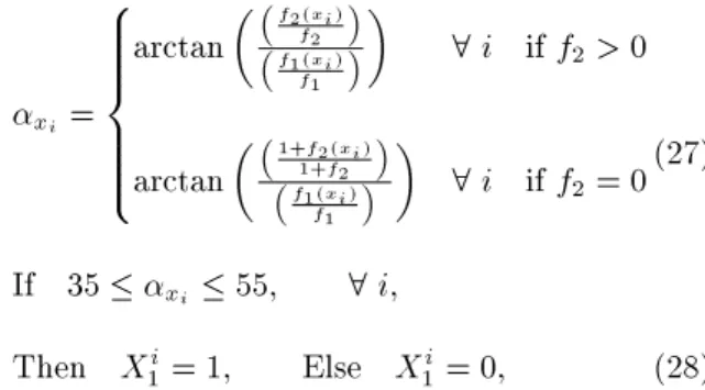
1. The rst provision: The decision-makers require
schedules with respect to the trade-o between various objectives. Figure 1 presents the acceptable trade-o between the objectives by angle (). The angle of the ith neighborhood solution (xi), called
xi, is computed as given in Eq. (27), and the
rst provision is designed as given in Eq. (28). According to the rst provision, xi at the interval
of 35 to 55 (4510) degrees is proper and condition is satised:
xi=
8 > > > > > < > > > > > :
arctan
f2(xi) f2
f1(xi)
f1
8 i if f2> 0
arctan
1+f2(xi) 1+f2
f1(xi)
f1
8 i if f2= 0(27)
If 35 xi 55; 8 i;
Then Xi
1= 1; Else X1i = 0; (28)
where f1(xi) and f2(xi) are the makespan and
total tardiness of the ith neighborhood solution,
Figure 1. A range of angle as an acceptable trade-o between the two objectives.
respectively. It is noted that several neighborhood solutions derived from the current solution (x0)
are generated. f1 and f2 are the lowest observed
makespan and total tardiness values, respectively, which can be updated after each iteration. To prevail over the trap of dealing with dierent measurement sizes of objective values, the value of each objective function should be normalized by dividing the actual objectives' values into the minimum objectives. In this respect, one is added to the denominator and numerator when f2is equal
to 0 (f2= 0);
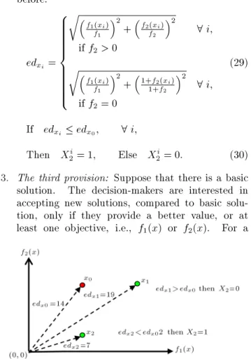
2. The second provision: The hope of decision-makers is to nd schedules close to the ideal point (0, 0). For this reason, the obtained solutions should converge towards the ideal point. Figure 2 presents the convergence of the ideal point by distance (ed). The distance between the ideal point and the ith neighborhood solution, called edxi, is computed
as given in Eq. (29), and the second provision is designed as given in Eq. (30). According to the second provision, if edxi has lower value of distance
between the ideal point and current solution (edx0),
then the condition for the corresponding solution is satised. Parameter denitions are presented as before.
edxi =
8 > > > > > > > > > < > > > > > > > > > : r
f1(xi)
f1
2
+f2(xi)
f2
2
8 i; if f2> 0
r
f1(xi)
f1
2
+1+f2(xi)
1+f2
2
8 i; if f2= 0
(29)
If edxi edx0; 8 i;
Then Xi
2= 1; Else X2i = 0: (30)
3. The third provision: Suppose that there is a basic solution. The decision-makers are interested in accepting new solutions, compared to basic solu-tion, only if they provide a better value, or at least one objective, i.e., f1(x) or f2(x). For a
Figure 2. A hypothetical example of distance.
bi-objective problem, this criterion is dened as given in Eq. (31). This criterion is one of the simplest acceptance criteria dened with decision-makers' comments. Similar to the mentioned cri-terion, the third provision is designed as given in Eq. (32). According to the third provision, if at least one objective of ith neighborhood solution (f1(xi) or f2(xi)) has lower value of the current
solution (f1(x0) or f2(x0)), then the condition for
the corresponding solution is satised:
f1(xi) < f1(x0); or f2(xi) < f2(x0); 8 i;
(31) If f1(xi)<f1(x0); or f2(xi)<f2(x0); 8 i;
Then Xi
3= 1; Else X3i = 0: (32)
4. The fourth provision: Researchers use Relative
Percentage Deviation (RPD) as a common perfor-mance measure. This criterion is shown in Eq. (33):
RPD = Algsol minsol
minsol ; (33)
where Algsol denotes the objective function value obtained for a given algorithm, minsol indicates
the best obtained value for objective function. It is clear that lower values of RPD are preferable. For a bi-objective problem, the RPD of the ith neighborhood solution, called RPDxi, is computed
as given in Eq. (34). Based on the mentioned criterion, the fourth provision is designed as given in Eq. (35). According to the fourth provision, if RPDxi has lower value of the current solution
(RPDx0), then the condition for the corresponding
solution is satised. Parameter denitions are
presented as before:
RPDxi =
8 > > > > > > < > > > > > > :
f1(xi) f1
f1 +
f2(xi) f2
f2 8 i;
If f2> 0
f1(xi) f1
f1 +
f2(xi) f2
1+f2 8 i;
If f2= 0
(34)
If RPDxi < RPDx0; 8 i;
Then Xi
4= 1; Else X4i = 0: (35)
5. The fth provision: One of the other views of
decision-makers is to minimize a convex combina-tion of objective funccombina-tions. For a bi-objective prob-lem, a convex combination of the ith neighborhood solution, called f(xi), is computed in Eq. (36).
Based on the mentioned function, the fth provision is designed as given in Eq. (37). According to
the fth provision, if f(xi) has lower value of the
current solution (f(x0)), then condition for the
corresponding solution is satised: f(xi) = ( f1(xi) + (1 ) f2(xi));
8 i; (36)
If f(xi) < f(x0); 8 i;
Then Xi
5= 1; Else X5i = 0: (37)
Note that the objectives are not normalized. Con-sequently, this criterion is sensitive to increasing and decreasing in the objective function with a larger value. The application of this criterion is important when objective values of the new solutions are close to the current solution. In the following, an example is provided to clarify. Suppose that the current solution is (10, 1500), and new solutions, x1 and x2, are (9, 1505) and
(11, 1495), respectively. According to the third provision, both new solutions are acceptable. If is set equal to 0.5, then objective functions (f(x)) are calculated as follows: f(x0) = 755, f(x1) = 757,
and f(x2) = 753. According to the fth provision,
only x2 is acceptable;
6. The sixth provision: Similar to the fth provision, the sixth provision is designed. Instead of actual values, the normalized objectives have been used in the provision. The normalized objectives are computed as given in Eq. (38):
f0
1(x) = ff1 1(x);
f0 2(x) =
8 > < > :
f2
f2(x) if f2> 0
1+f2
1+f2(x) if f2= 0 or f2(x) = 0
9 > = > ;:(38) The one is added to the denominator and numerator when the total tardiness or minimum total tardiness is equal to 0.
The total objective function of the ith neigh-borhood solution, called f0(x
i), is computed as
given in Eq. (39). Based on the mentioned function, the sixth provision is designed as given in Eq. (40). According to the sixth provision, if f0(xi) has lower
value of the current solution (f0(x0)), then the
condition for the corresponding solution is satised: f0(x
i) = ( f10(xi) + (1 ) f20(xi)) 1; (39)
If f0(x
i) < f0(x0) 8 i;
Then Xi
6= 1 Else X6i = 0: (40)
7. The seventh provision: The total deviation of
each new solution of the current solution, called Deviationxi is computed as given in Eq. (41). The
result of this deviation can be positive or negative. Two cases represent a negative value as follows:
(a) Both objectives are worse;
(b) One of the objectives is better and the other is worse;
however, the negative deviation will dominate the positive deviation. Two cases represent a positive value as follows:
(a) Both objectives are better;
(b) One of objectives is better and the other is worse;
however, the positive deviation will dominate the
negative deviation. Consequently, the positive
results are more suitable. In fact, decision-makers are interested in achieving new solutions with the positive values of the total deviation. Based on the mentioned criterion, the seventh provision is designed as given in Eq. (42). According to the seventh provision, if Deviationxi has a positive
value, then the condition for the corresponding solution is satised:
Deviationxi=
f1(x0) f1(xi)
f1(x0) +
f2(x0) f2(xi)
(1 + f2(x0)) ;
8i; (41)
If deviationxi > 0; 8 i;
Then Xi
7= 1; Else X7i = 0: (42)
Now, the dierence between the third and seventh provisions is described. In the third provision, decision-makers accept new solutions only if they provide a better value, even at least one objective. In the seventh provision, rst, at least one of objectives provide a better value. Then, the pos-itive deviation dominates the negative deviation. In the progress, the dierence between the fourth and seventh provisions is described. In the fourth provision, old and new solutions are measured to a minimum value separately. In the seventh provi-sion, old and new solutions are measured directly together;
8. The proposed objective function: Based on the seven provisions described, a new objective function is dened in terms of requests, comments, and view-points of the decision-makers as follows (Eq. (43)):
Total objective function = maximizing Z; Zi= Xi
1+ X2i+ X3i+ X4i+ X5i+ X6i+ X7i;
8 i; s.t.: Xi
j =
8 > < > :
1 If jth condition of neighborhood solution ith is satised
0 Otherwise
j = 1; 2; ; 7: (43)
Some interesting points are presented as follows:
- First, the objective function is converted from the minimizing into the maximizing;
- Second, seven additional traits are added to the objective function;
- Third, decision-makers express the features
added to the objective function;
- Fourth, the objective function will serve as a \template" to/from which the assumptions and constraints will be added or removed to describe dierent objective function variants.
4.2. The proposed algorithm pseudo code The pseudo code of the VNS-PA algorithm applied in this paper is now presented as follows.
Initialization
Encoding: Integer coding is used in this research for the representation of a solution. In this kind of representation, a single row array of the size equal to the number of the jobs to be scheduled is formed. The value of the rst element of the array shows which job is scheduled rst. The second value shows the job scheduled, and so on. For an example, a solution is generated according integer coding as [3 1 4 2 5] for a problem with ve jobs (n = 5);
Input parameters: Maximum number of
itera-tion of inner loop (max it); the weighting coe-cients ( 2 f0:25; 0:5; 0:75g);
Draw an initial solution, x0: The initial
solution is generated in a random way from the search space;
Evaluate f1(x0) and f2(x0): f1(x0) is the
makespan; f2(x0) is the total tardiness of initial
solution;
Set: q = 1, archive (q) = fx0g, f1 = f1(x0), and
f2= f2(x0).
For it=1: max it, %maximum number of iteration inner loop is max it
NSS = 1 While NSS < 4
Follow Steps 1 to 3, respectively.
Step 1: Generate neighborhood solutions:
If NSS = 1, perform the swap move on x0 and
generate n solutions;
If NSS = 2, perform the shift move on x0 and
generate n solutions;
If NSS = 3, perform the inversion move on x0and
generate n solutions;
Evaluate f1(xi) and f2(xi) as new solutions in the
neighborhood of x0;
Update f1 and f2 as f1 = minff1; f1(xi)i =
1; 2; ; ng, f2= minff2; f2(xi)i = 1; 2; ; ng.
Step 2: Consider provisions and calculate Z for each neighborhood solution.
Consider conditions (Eqs. (28), (30), (32), (35), (37), (40), and (42)) for each neighborhood solution:
If 35 xi 55; 8 i;
Then Xi
1= 1; Else X1i= 0;
If edxi edx0; 8 i;
Then Xi
2= 1; Else X2i= 0;
If 8 > < > :
f1(xi) < f1(x0)
or
f2(xi) < f2(x0)
8 i;
Then Xi
3= 1; Else X3i= 0
If RPDxi < RPDx0; 8 i;
Then Xi
4= 1; Else X4i= 0;
If f(xi) < f(x0); 8 i;
Then Xi
5= 1; Else X5i= 0;
If f0(x
i) < f0(x0); 8 i;
Then Xi
6= 1; Else X6i= 0;
If Deviation xi> 0; 8 i;
Then Xi
Calculate objective function Z (Eq. (43)) for each neighborhood solution:
Zi= Xi
1+ X2i+ X3i+ X4i+ X5i+ X6i+ X7i;
8 i; s.t.:
Xi j j=1;2; ;7=
8 > > > > > > < > > > > > > :
1 If jth condition of
neighborhood solution ith is satised
0 Otherwise Step 3: Decision-making
If 9k that Zk = max(Zi; 8 i) 4 (accept
57.1% of the cited conditions), Then x0 = the corresponding solution with
maximal number of provisions (or x0 xk)
q = q + 1; Archive (q) = fxkg
NSS = NSS Else
NSS = NSS + 1; End If
End While End For
Select one of the archived solutions according to provi-sions.
5. Computational experiments
This section contains the method for generating data sets, runs these data sets by the proposed algorithm, full enumeration algorithm, and algorithm in the lit-erature, and expresses the results of the validation of the proposed model, the proposed algorithm; then, the results of the eciency of the proposed algorithm are presented.
5.1. Test problems
The data required for a problem consist of the num-ber of re-entrants, jobs, machines per stage, stages, processing times, due dates, setup times, and learning indices. The designing range of the levels of each factor is illustrated, as shown in Table 1. The number of machines, processing times, and setup times are randomly generated from a discrete uniform distribu-tion, as described in Table 1. This table includes 4 categories of problems: (1) special small, (2) small, (3) medium, and (4) large problems. Special small problems are designed to assess the validity of the proposed algorithm. The specic name is given to these problems because they cover small problems of single machine, parallel machine, ow shop, and two-stage HFS. To demonstrate the eectiveness of the proposed VNS-PA compared to algorithm in the literature, the experiments are conducted on three sizes of problems: small, medium, and large. The twenty-four problems are produced for the special small problems. Ten problems are produced for the small, medium, and large problems. Learning indices {0.152 and {0.514 are selected with respect to the learning curve of 90% and 70%, respectively. In general, all problems are tested with regard to the level of learning indices. To generate due dates of all n jobs, the following steps are proposed:
- Compute the total processing time of each job on all g stages:
Pj = L
X
l=1 g
X
t=1
Pt
jl; 8 j 2 n: (44)
- Compute average setup time for all possible subse-quent jobs and sum it for all g stages:
Sj = L
X
l=1 g
X
t=1
0 B B @
n
P
k=1S t kjl
n 1 C C
A ; 8 j 2 n: (45)
Table 1. Factors and their levels.
Factor Levels
Special small Small Medium Large
Number of jobs (n) 5; 7; and10 10; 15; and 20 25; 30; and 35 40; 50; and 60 Number of stages (g) 1; and 2 5; 7; and 10 10; 12; and 15 15; 17; and 20 Number of re-entrants (L) 1; and 2 1; and 2 2; and 3 3; and 4 Number of machines (mt) 1; and 3 Uniform (1, 3) Uniform (1, 6) Uniform (1, 9) Processing times (P ) Uniform (10, 20) Uniform (10, 20) Uniform (10, 40) Uniform (10, 100) Setup times (S) Uniform (3, 6) Uniform (3, 6) Uniform (5, 10) Uniform (11, 22)
- Determine a due date for each job: dj=(Pj+Sj)
0 B B @
max
mt t2g
g
1 C C
A(1+random3);
8 j 2 n; (46)
where random is a random number from a uniform distribution over range (0, 1).
5.2. The validation of proposed model
To demonstrate the validation of the proposed model, the experiments were conducted on ve special small problems. Each example is solved by the full enu-meration algorithm and LINGO software. Solving a problem with enumeration algorithm includes trying all the possibilities that exist with manual calculations. Details of the special small-sized problems and results are shown in Table 2. Because the process of the solution is time consuming, the runtime was limited to two hours.
It is obvious from the table that the optimal solu-tion has been obtained for the rst problem. This result demonstrates the ability of the proposed approach to model the problem and nd an optimal solution. Due to time constraints, a gap between the optimal solution and obtained solution exists for other problems. The results show that error increases signicantly when the dimensions are slightly larger. Thus, meta-heuristic methods must be used to solve problems.
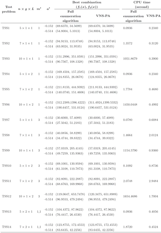
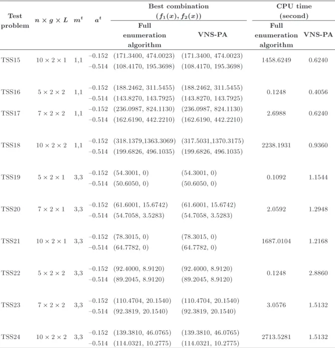
5.3. The validation of the proposed algorithm To demonstrate the validation of the proposed VNS-PA, the experiments were conducted on special small problems. The full enumeration algorithm is used to nd the optimal solution to every problem. Details of special small-sized problems and results are shown in Table 3. According to the table, the rst column indicates the abbreviation codes of each test problem, the second and third columns describe the details of problems (number of jobs number of stages number of re-entrants, and number of machines per stage), the fourth describes learning indices, the fth describes the best value of objectives for the proposed
objective function, and the last column describes the average CPU time (second unit).
It is noticeable that the maximum number of iteration of inner loop, called max it, is the only parameter of the proposed algorithm and set max it = 10. Based on the results given in Table 3, the following observations can be drawn.
Due to the proposed objective function, the pro-posed algorithm is able to nd the optimal schedule in 93.75% of the cases. This result indicates that the proposed algorithm has very high reliability (excellent performance) to solve the problems. The proposed algorithm is able to solve the problems in the length of the interval from 0.2340 to 2.9484 seconds. The full enumeration algorithm has spent the interval from 0.0780 to 2713.5281 seconds. This result indicates that the proposed algorithm has a signicant speed in solving the problem. The proposed algorithm is able to nd the optimal schedule in 58.33% of the cases faster than the full enumeration algorithm.
5.4. Numerical result
To demonstrate the eciency of the proposed VNS-PA, the Simulated Annealing (SA) algorithm proposed by Mousavi et al. [12] is used. It is noticeable that all of algorithms are implemented in MATLAB 2009a, which is a special mathematical computation language and run on a PC with 2.30 GHz Intel Core and 4 GB of RAM memory. To show the eciency and eectiveness of the proposed algorithm in comparison with a SA, computational experiments were carried out on various test problems (i.e., small, medium, and large). The three replications of each problem size have been performed since there are some random conditions when applying the algorithm.
Tables 4 to 6 show the results of the implementa-tion of algorithms on various problems. In addiimplementa-tion, the rst column indicates the abbreviation codes of each test problem, the second and third columns describe the weights of sets f0:25; 0:5; and 0:75g and learning indices of sets f 0:152 and 0:514g, the fourth column describes the best combination of objectives for each algorithm, the fth column describes the value of the proposed objective function (Eq. (42)) for each algorithm, compared to their solutions in the fourth
Table 2. Details of special small-sized problems and results of LINGO. Test
problem
Details of problems at Optimal solution (f1(x); f2(x))
LINGO results
(f1(x); f2(x)) Gap %
n g L mt
1 10 1 1 1 {0.152 (151.2996, 351.0591) Optimal solution 0 2 10 2 1 1, 1 {0.152 (171.3400, 474.0023) (185.1399, 573.1197) 17.50 3 10 2 1 3, 3 {0.152 (78.3015, 0) (88.7881, 38.9454) 63.13 4 10 2 2 3, 3 {0.152 (139.3810, 46.0765) (159.2371, 192.8482) 89.85 5 10 2 3 3, 3 {0.152 (242.6945, 516.8420) No solution Innite
Table 3. Details of special small-sized problems and results of algorithms. Test
problem n g L m t at
Best combination (f1(x); f2(x))
CPU time (second) Full
enumeration algorithm
VNS-PA
Full enumeration
algorithm
VNS-PA
TSS1 5 1 1 1 {0.152 (69.6370, 34.5699) (69.6370, 34.5699) 0.0936 0.2340 {0.514 (54.8004, 5.1013) (54.8004, 5.1013)
TSS2 7 1 1 1 {0.152 (94.9153, 113.8748) (94.9153, 113.8748) 1.3572 0.3120 {0.514 (63.0024, 31.9535) (63.0024, 31.9535)
TSS3 10 1 1 1 {0.152 (151.2996, 351.0591) (151.2996, 351.0591) 1051.8679 0.3900 {0.514 (90.7567, 108.1328) (90.7567, 108.1328)
TSS4 5 1 2 1 {0.152 (169.4504, 157.2585) (169.4504, 157.2585) 0.0936 0.2340 {0.514 (124.8355, 26.0678) (124.8355, 26.0678)
TSS5 7 1 2 1 {0.152 (211.8133, 444.9392) (211.8133, 444.9392) 1.7784 0.4680 {0.514 (140.0740, 151.4606) (140.0740, 151.4606)
TSS6 10 1 2 1 {0.152 (312.2389,1396.4222) (311.4924,1399.5332) 1450.0448 0.4992 {0.514 (190.6457, 531.0124) (190.6457, 531.0124)
TSS7 5 1 1 3 {0.152 (30.6000, 57.4089) (30.6000, 57.4089) 0.0780 0.6084 {0.514 (27.5042, 51.2183) (27.5042, 51.2183)
TSS8 7 1 1 3 {0.152 (40.0856, 58.8299) (40.0856, 58.8299) 1.4664 2.0124 {0.514 (34.4744, 39.8322) (34.4744, 39.8322)
TSS9 10 1 1 3 {0.152 (57.0319, 205.4145) (57.0319, 205.4145) 1154.5790 0.9360 {0.514 (49.7259, 135.9363) (49.7259, 135.9363)
TSS10 5 1 2 3 {0.152 (69.1001, 130.9594) (69.1001, 130.9594) 0.1092 0.8736 {0.514 (61.3108, 110.7873) (61.3108, 110.7873)
TSS11 7 1 2 3 {0.152 (82.8091, 222.2887) (82.8091, 222.2887) 2.0748 2.9484 {0.514 (68.6763, 169.9968) (68.6763, 169.9968)
TSS12 10 1 2 3 {0.152 (119.0647, 653.7478) (120.3475, 651.8989) 1654.4686 1.7004 {0.514 (96.9553, 479.2494) (96.9553, 479.2494)
TSS13 5 2 1 1,1 {0.152 (104.4372, 87.9622) (104.4372, 87.9622) 0.0936 0.4056 {0.514 (76.4417, 26.4530) (76.4417, 26.4530)
TSS14 7 2 1 1,1 {0.152 (123.8755, 172.4553) (123.8755, 172.4553) 1.8720 0.4524 {0.514 (83.6435, 42.2256) (83.6435, 42.2256)
Table 3. Details of special small-sized problems and results of algorithms (continued). Test
problem n g L m t at
Best combination (f1(x); f2(x))
CPU time (second) Full
enumeration algorithm
VNS-PA
Full enumeration
algorithm
VNS-PA
TSS15 10 2 1 1,1 {0.152 (171.3400, 474.0023) (171.3400, 474.0023) 1458.6249 0.6240 {0.514 (108.4170, 195.3698) (108.4170, 195.3698)
TSS16 5 2 2 1,1 {0.152 (188.2462, 311.5455) (188.2462, 311.5455) 0.1248 0.4056 {0.514 (143.8270, 143.7925) (143.8270, 143.7925)
TSS17 7 2 2 1,1 {0.152 (236.0987, 824.1130) (236.0987, 824.1130) 2.6988 0.6240 {0.514 (162.6190, 442.2210) (162.6190, 442.2210)
TSS18 10 2 2 1,1 {0.152 (318.1379,1363.3069) (317.5031,1370.3175) 2238.1931 0.9360 {0.514 (199.6826, 496.1035) (199.6826, 496.1035)
TSS19 5 2 1 3,3 {0.152 (54.3001, 0) (54.3001, 0) 0.1092 1.1544 {0.514 (50.6050, 0) (50.6050, 0)
TSS20 7 2 1 3,3 {0.152 (61.6001, 15.6742) (61.6001, 15.6742) 2.0592 1.2948 {0.514 (54.7058, 3.5283) (54.7058, 3.5283)
TSS21 10 2 1 3,3 {0.152 (78.3015, 0) (78.3015, 0) 1687.0104 1.2168 {0.514 (64.7782, 0) (64.7782, 0)
TSS22 5 2 2 3,3 {0.152 (92.4000, 8.9120) (92.4000, 8.9120) 0.1248 2.8860 {0.514 (89.2045, 8.9120) (89.2045, 8.9120)
TSS23 7 2 2 3,3 {0.152 (110.4704, 20.1540) (110.4704, 20.1540) 3.0576 1.5132 {0.514 (92.3819, 20.1540) (92.3819, 20.1540)
TSS24 10 2 2 3,3 {0.152 (139.3810, 46.0765) (139.3810, 46.0765) 2713.5281 1.5132 {0.514 (114.0321, 10.2775) (114.0321, 10.2775)
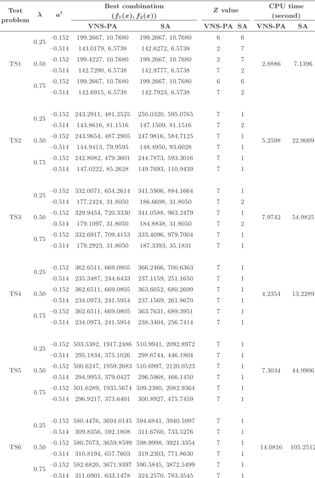
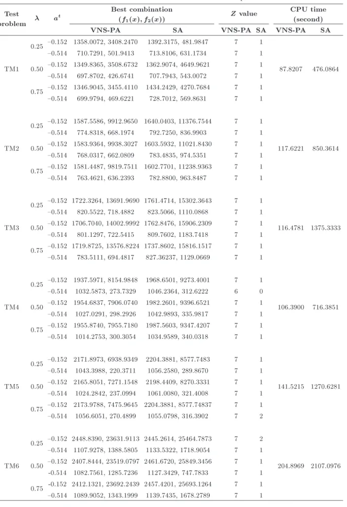
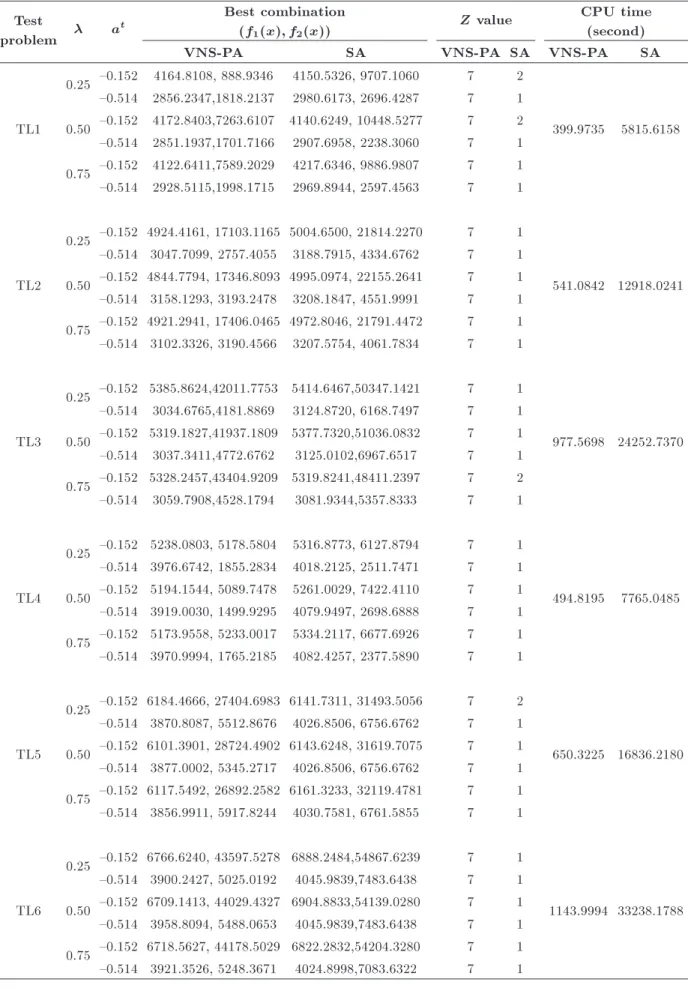
column, and the last column describes the average CPU time (second unit). The last two columns in these tables are applied to compare the results.
Time cost is an important factor when comparing dierent algorithms. According to a report in the last column of Tables 4 to 6, the proposed algorithm is able to solve the small, medium, and large problems in the length of the interval [2.132, 14.0816], [37.4037, 204.8969], and [399.9735, 2740.6281] seconds,
respec-tively. The SA algorithm has spent the interval
from 7.1396 to 105.2512, 476.0864 to 2107.0976, and 5372.7861 to 33238.1788 seconds for small, medium, and large problems, respectively. This result indicates that the proposed algorithm in comparison with other
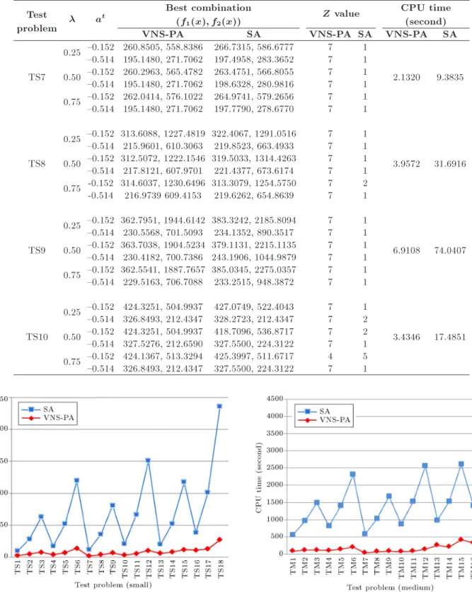
algorithm has a signicant speed in solving the prob-lem. In addition, Figures 3 to 5 plot the computational times of the two algorithms for small, medium, and large problems, respectively. It can be seen that the computational times or the running times of VNS-PA are considerably less than SA.
In order to evaluate the nal solutions' quality of each algorithm, column `Z value' in Tables 4 to 6 is used. In fact, this column is the value of the proposed objective function (Eq. (42)). It is known that a new objective function is designed in terms of requests, comments, and viewpoints of the decision-makers. As noted, the seven additional traits are added to the proposed objective function. Consequently, the value
Table 4. Results of VNS-PA and SA for small-sized problems. Test
problem at
Best combination
(f1(x); f2(x)) Z value
CPU time (second)
VNS-PA SA VNS-PA SA VNS-PA SA
TS1
0.25 {0.152 199.2667, 10.7680 199.2667, 10.7680 6 6
2.8886 7.1396 {0.514 143.0179, 6.5738 142.6272, 6.5738 2 7
0.50 {0.152 199.4227, 10.7680 199.2667, 10.7680 2 7 {0.514 142.7290, 6.5738 142.9777, 6.5738 7 2 0.75 {0.152 199.2667, 10.7680 199.2667, 10.7680 6 6 {0.514 142.6915, 6.5738 142.7923, 6.5738 7 2
TS2
0.25 {0.152 243.2911, 481.2525 250.0320, 595.0765 7 1
5.2598 22.9009 {0.514 143.8616, 81.1516 147.1509, 81.1516 7 2
0.50 {0.152 243.9654, 487.2905 247.9816, 584.7125 7 1 {0.514 144.9413, 79.9595 148.4950, 93.6028 7 1 0.75 {0.152 242.8082, 479.3601 244.7873, 593.3016 7 1 {0.514 147.0222, 85.2628 149.7693, 110.9439 7 1
TS3
0.25 {0.152 332.0071, 654.2614 341.5906, 884.1664 7 1
7.9742 54.9825 {0.514 177.2424, 31.8050 186.6698, 31.8050 7 2
0.50 {0.152 329.9454, 720.3330 341.0588, 963.2479 7 1 {0.514 179.1097, 31.8050 184.8838, 31.8050 7 2 0.75 {0.152 332.6917, 709.4153 333.4096, 979.7004 7 1 {0.514 179.2923, 31.8050 187.3393, 35.1831 7 1
TS4
0.25 {0.152 362.6511, 669.0805 366.2466, 700.6363 7 1
4.2354 13.2289 {0.514 235.3487, 244.6433 237.1159, 251.1650 7 1
0.50 {0.152 362.6511, 669.0805 363.6052, 680.2699 7 1 {0.514 234.0973, 241.5954 237.1569, 261.8670 7 1 0.75 {0.152 362.6511, 669.0805 363.7631, 689.3951 7 1 {0.514 234.0973, 241.5954 238.3404, 256.7414 7 1
TS5
0.25 {0.152 503.5382, 1917.2486 510.9941, 2092.8972 7 1
7.3034 44.9906 {0.514 295.1834, 375.1026 298.6744, 446.1804 7 1
0.50 {0.152 500.6247, 1959.2683 510.6997, 2120.0523 7 1 {0.514 294.9953, 379.0427 296.5968, 466.1450 7 1 0.75 {0.152 501.6289, 1935.5674 509.2380, 2082.9364 7 1 {0.514 296.9217, 373.6401 300.8927, 475.7459 7 1
TS6
0.25 {0.152 580.4476, 3694.0145 594.6841, 3940.5997 7 1
14.0816 105.2512 {0.514 309.8356, 592.1808 311.6760, 733.5276 7 1
0.50 {0.152 580.7073, 3659.8599 598.9998, 3921.3354 7 1 {0.514 310.8194, 657.7603 319.2303, 771.8630 7 1 0.75 {0.152 582.6820, 3671.9397 590.5845, 3872.5499 7 1 {0.514 311.6901, 633.1478 324.2570, 783.3545 7 1
Table 4. Results of VNS-PA and SA for small-sized problems (continued). Test
problem a
t Best combination
(f1(x); f2(x)) Z value
CPU time (second)
VNS-PA SA VNS-PA SA VNS-PA SA
TS7
0.25 {0.152 260.8505, 558.8386 266.7315, 586.6777 7 1
2.1320 9.3835 {0.514 195.1480, 271.7062 197.4958, 283.3652 7 1
0.50 {0.152 260.2963, 565.4782 263.4751, 566.8055 7 1 {0.514 195.1480, 271.7062 198.6328, 280.9816 7 1 0.75 {0.152 262.0414, 576.1022 264.9741, 579.2656 7 1 {0.514 195.1480, 271.7062 197.7790, 278.6770 7 1
TS8
0.25 {0.152 313.6088, 1227.4819 322.4067, 1291.0516 7 1
3.9572 31.6916 {0.514 215.9601, 610.3063 219.8523, 663.4933 7 1
0.50 {0.152 312.5072, 1222.1546 319.5033, 1314.4263 7 1 {0.514 217.8121, 607.9701 221.4377, 673.6174 7 1 0.75 -0.152 314.6037, 1230.6496 313.3079, 1254.5750 7 2 -0.514 216.9739 609.4153 219.6262, 654.8639 7 1
TS9
0.25 {0.152 362.7951, 1944.6142 383.3242, 2185.8094 7 1
6.9108 74.0407 {0.514 230.5568, 701.5093 234.1352, 890.3517 7 1
0.50 {0.152 363.7038, 1904.5234 379.1131, 2215.1135 7 1 {0.514 230.4182, 700.7386 243.1906, 1044.9879 7 1 0.75 {0.152 362.5541, 1887.7657 385.0345, 2275.0357 7 1 {0.514 229.5163, 706.7088 233.2515, 948.3872 7 1
TS10
0.25 {0.152 424.3251, 504.9937 427.0749, 522.4043 7 1
3.4346 17.4851 {0.514 326.8493, 212.4347 328.2723, 212.4347 7 2
0.50 {0.152 424.3251, 504.9937 418.7096, 536.8717 7 2 {0.514 327.5276, 212.6590 327.5500, 224.3122 7 1 0.75 {0.152 424.1367, 513.3294 425.3997, 511.6717 4 5 {0.514 326.8493, 212.4347 327.5500, 224.3122 7 1
Figure 3. The computational times of VNS-PA and SA for small-sized problems.
of the proposed objective function demonstrates the number of provisions satised. It is obvious from this column that the proposed algorithm produces solutions more acceptable than others to the decision-maker in most cases.
Figure 4. The computational times of VNS-PA and SA for medium-sized problems.
A graphical representation is provided to demon-strate output results of the VNS-PA and SA (Figure 6). This gure shows the obtained solutions of VNS-PA and SA algorithms over twenty runs for TM8 problem. It is observed in this gure that the obtained
Table 5. Results of VNS-PA and SA for medium-sized problems. Test
problem at
Best combination
(f1(x); f2(x)) Z value
CPU time (second)
VNS-PA SA VNS-PA SA VNS-PA SA
TM1
0.25 {0.152 1358.0072, 3408.2470 1392.3175, 481.9847 7 1
87.8207 476.0864 {0.514 710.7291, 501.9413 713.8106, 631.1734 7 1
0.50 {0.152 1349.8365, 3508.6732 1362.9074, 4649.9621 7 1 {0.514 697.8702, 426.6741 707.7943, 543.0072 7 1 0.75 {0.152 1346.9045, 3455.4110 1434.2429, 4270.7684 7 1 {0.514 699.9794, 469.6221 728.7012, 569.8631 7 1
TM2
0.25 {0.152 1587.5586, 9912.9650 1640.0403, 11376.7544 7 1
117.6221 850.3614 {0.514 774.8318, 668.1974 792.7250, 836.9903 7 1
0.50 {0.152 1583.9364, 9938.3027 1603.5932, 11021.8430 7 1 {0.514 768.0317, 662.0809 783.4835, 974.5351 7 1 0.75 {0.152 1581.4487, 9819.7511 1602.7701, 11238.9363 7 1 {0.514 763.4621, 636.2393 782.8800, 963.8487 7 1
TM3
0.25 {0.152 1722.3264, 13691.9690 1761.4714, 15302.3643 7 1
116.4781 1375.3333 {0.514 820.5522, 718.4882 823.5066, 1110.0868 7 1
0.50 {0.152 1706.7040, 14002.9992 1762.8476, 15906.2309 7 1 {0.514 801.1297, 722.5415 809.7602, 1183.7418 7 1 0.75 {0.152 1719.8725, 13576.8224 1737.8602, 15816.1517 7 1 {0.514 783.5111, 694.4817 827.36237, 1129.0669 7 1
TM4
0.25 {0.152 1937.5971, 8154.9848 1968.6501, 9273.4001 7 1
106.3900 716.3851 {0.514 1032.5873, 273.7329 1046.2364, 312.6222 6 0
0.50 {0.152 1954.6837, 7906.0740 1982.2601, 9396.6521 7 1 {0.514 1027.0291, 298.2926 1042.9893, 335.9817 7 1 0.75 {0.152 1955.8740, 7955.7180 1987.5603, 9347.4207 7 1 {0.514 1014.2753, 300.3054 1034.9589, 340.0318 7 1
TM5
0.25 {0.152 2171.8973, 6938.9349 2204.3881, 8577.7483 7 1
141.5215 1270.6281 {0.514 1043.3988, 220.3711 1056.2580, 289.8670 7 1
0.50 {0.152 2165.8051, 7271.1548 2198.4409, 8270.3331 7 1 {0.514 1024.2842, 237.0994 1061.0080, 321.4008 7 1 0.75 {0.152 2173.9788, 7475.9645 2204.3881, 8577.74837 7 1 {0.514 1056.6051, 270.4899 1055.0798, 316.3902 7 2
TM6
0.25 {0.152 2448.8390, 23631.9113 2445.2614, 25464.7873 7 2
204.8969 2107.0976 {0.514 1107.9278, 1388.5805 1133.5322, 1718.9054 7 1
0.50 {0.152 2407.8444, 23519.0797 2461.6720, 25849.3456 7 1 -0.514 1082.7561, 1285.7236 1127.3429, 747.7833 7 1 0.75 -0.152 2412.1321, 23692.2439 2457.4201, 25693.1264 7 1 {0.514 1089.9052, 1343.1999 1139.7435, 1678.2789 7 1
Table 5. Results of VNS-PA and SA for medium-sized problems (continued). Test
problem a
t Best combination(f1(x); f2(x)) Z value CPU time(second)
VNS-PA SA VNS-PA SA VNS-PA SA
TM7
0.25 {0.152 1510.5763, 5235.1305 1543.1791, 6681.8272 7 1
37.4037 544.2458 {0.514 926.7607, 1092.6267 947.4376, 1296.5893 7 1
0.50 {0.152 1510.9277, 5398.6588 1534.4259, 6399.7784 7 1 {0.514 935.4230, 1133.4456 937.1943, 1446.3046 7 1 0.75 {0.152 1503.1919, 5293.9026 1543.0130, 6749.0115 7 1 {0.514 935.0112, 1112.1764 978.6252, 1331.9636 7 1
TM8
0.25 {0.152 1650.2158, 9894.0778 1687.5328, 11584.0113 7 1
73.9600 960.4357 {0.514 940.1271, 1413.0879 953.0611, 2186.4549 7 1
0.50 {0.152 1639.7358, 10091.1065 1705.8712, 11672.9533 7 1 {0.514 952.4433, 1412.7473 987.2651, 2345.4782 7 1 0.75 {0.152 1643.3910, 9874.9129 1686.6839, 11686.5147 7 1 {0.514 953.7051, 1540.7814 947.1948, 2000.8256 7 2
TM9
0.25 {0.152 1764.9555, 12256.6683 1828.3645, 14726.4105 7 1
87.3475 1592.3125 {0.514 942.2798, 228.4465 963.0248, 510.0353 7 1
0.50 {0.152 1762.2872, 13013.2504 1829.1604, 14726.9819 7 1 {0.514 953.4593, 280.4752 934.6274, 426.4481 7 2 0.75 {0.152 1774.8750, 12595.7547 1802.9873, 14916.5601 7 1 {0.514 934.2507, 270.4154 943.95911, 341.4312 7 1
TM10
0.25 {0.152 2162.4255, 8277.5059 2212.8799, 9453.2599 7 1
70.6346 803.4519 {0.514 1271.5181, 1217.9128 1289.9953, 1516.7192 7 1
0.50 {0.152 2142.3687, 8348.9381 2220.2212, 9744.1022 7 1 {0.514 1273.4044, 1034.0347 1287.3140, 1485.9365 7 1 0.75 {0.152 2147.2849, 8014.8205 2170.8716, 9417.6667 7 1 {0.514 1273.6014, 1062.6905 1278.8012, 1555.42840 7 1
Figure 5. The computational times of VNS-PA and SA for large-sized problems.
solutions of SA algorithm have a trade-o between various objectives (rst provision); however. other features (provisions 2 to 7) are not satised. This gure
Figure 6. The generated combinations of VNS-PA and SA for TM8 problem.
illustrates and conrms the conclusion derived from the numerical results based on the performance criterion.
In order to visualize the performance of the two algorithms, the archived solutions from one run of each algorithm are selected to provide a graphical represen-tation of the medium-sized problem (Figures 7 and 8).
Table 6. Results of VNS-PA and SA for large-sized problems. Test
problem at
Best combination
(f1(x); f2(x)) Z value
CPU time (second)
VNS-PA SA VNS-PA SA VNS-PA SA
TL1
0.25 {0.152 4164.8108, 888.9346 4150.5326, 9707.1060 7 2
399.9735 5815.6158 {0.514 2856.2347,1818.2137 2980.6173, 2696.4287 7 1
0.50 {0.152 4172.8403,7263.6107 4140.6249, 10448.5277 7 2 {0.514 2851.1937,1701.7166 2907.6958, 2238.3060 7 1 0.75 {0.152 4122.6411,7589.2029 4217.6346, 9886.9807 7 1 {0.514 2928.5115,1998.1715 2969.8944, 2597.4563 7 1
TL2
0.25 {0.152 4924.4161, 17103.1165 5004.6500, 21814.2270 7 1
541.0842 12918.0241 {0.514 3047.7099, 2757.4055 3188.7915, 4334.6762 7 1
0.50 {0.152 4844.7794, 17346.8093 4995.0974, 22155.2641 7 1 {0.514 3158.1293, 3193.2478 3208.1847, 4551.9991 7 1 0.75 {0.152 4921.2941, 17406.0465 4972.8046, 21791.4472 7 1 {0.514 3102.3326, 3190.4566 3207.5754, 4061.7834 7 1
TL3
0.25 {0.152 5385.8624,42011.7753 5414.6467,50347.1421 7 1
977.5698 24252.7370 {0.514 3034.6765,4181.8869 3124.8720, 6168.7497 7 1
0.50 {0.152 5319.1827,41937.1809 5377.7320,51036.0832 7 1 {0.514 3037.3411,4772.6762 3125.0102,6967.6517 7 1 0.75 {0.152 5328.2457,43404.9209 5319.8241,48411.2397 7 2 {0.514 3059.7908,4528.1794 3081.9344,5357.8333 7 1
TL4
0.25 {0.152 5238.0803, 5178.5804 5316.8773, 6127.8794 7 1
494.8195 7765.0485 {0.514 3976.6742, 1855.2834 4018.2125, 2511.7471 7 1
0.50 {0.152 5194.1544, 5089.7478 5261.0029, 7422.4110 7 1 {0.514 3919.0030, 1499.9295 4079.9497, 2698.6888 7 1 0.75 {0.152 5173.9558, 5233.0017 5334.2117, 6677.6926 7 1 {0.514 3970.9994, 1765.2185 4082.4257, 2377.5890 7 1
TL5
0.25 {0.152 6184.4666, 27404.6983 6141.7311, 31493.5056 7 2
650.3225 16836.2180 {0.514 3870.8087, 5512.8676 4026.8506, 6756.6762 7 1
0.50 {0.152 6101.3901, 28724.4902 6143.6248, 31619.7075 7 1 {0.514 3877.0002, 5345.2717 4026.8506, 6756.6762 7 1 0.75 {0.152 6117.5492, 26892.2582 6161.3233, 32119.4781 7 1 {0.514 3856.9911, 5917.8244 4030.7581, 6761.5855 7 1
TL6
0.25 {0.152 6766.6240, 43597.5278 6888.2484,54867.6239 7 1
1143.9994 33238.1788 {0.514 3900.2427, 5025.0192 4045.9839,7483.6438 7 1
0.50 {0.152 6709.1413, 44029.4327 6904.8833,54139.0280 7 1 {0.514 3958.8094, 5488.0653 4045.9839,7483.6438 7 1 0.75 {0.152 6718.5627, 44178.5029 6822.2832,54204.3280 7 1 {0.514 3921.3526, 5248.3671 4024.8998,7083.6322 7 1
Table 6. Results of VNS-PA and SA for large-sized problems (continued). Test
problem a
t Best combination(f1(x); f2(x)) Z value CPU time(second)
VNS-PA SA VNS-PA SA VNS-PA SA
TL7
0.25 {0.152 6246.4658, 45464.4212 6446.4307, 53745.4553 7 1
1364.8942 6464.4941 {0.514 3406.0145, 8823.4279 3554.3961, 11925.3353 7 1
0.50 {0.152 6237.0777, 45944.7375 6392.7104, 54142.9377 7 1 {0.514 3396.0878, 8714.8155 3542.5495, 11865.5127 7 1 0.75 {0.152 6249.8465, 46375.5315 6461.7802, 54677.5356 7 1 {0.514 3350.7780, 8626.9597 3593.1496, 11313.1816 7 1
TL8
0.25 {0.152 7799.8223,102904.7309 8053.6935,111465.6123 7 1
2078.8277 10958.0197 {0.514 3504.3149, 10464.9499 3584.2051,13289.3836 7 1
0.50 {0.152 7768.6782,103675.1357 7985.6674,112430.6504 7 1 {0.514 3453.8425, 10735.9776 3598.5267,13416.4172 7 1 0.75 {0.152 7808.7714,105051.7819 7896.8719,110282.3235 7 1 {0.514 3438.1813,10881.6987 3509.7262,12156.9936 7 1
TL9
0.25 {0.152 8608.6794,140797.9846 8737.4097,150944.8927 7 1
2740.6281 20061.9885 {0.514 3614.3819, 4511.8407 3643.3332,5593.0288 7 1
0.50 {0.152 8717.7292,144991.9183 8788.1980,150679.6168 7 1 {0.514 3593.1215, 3818.4760 3643.3332, 5593.0288 7 1 0.75 {0.152 8615.7452,143325.4396 8826.6965,154839.6608 7 1 {0.514 3582.6382, 4139.2756 3703.5108, 5861.5393 7 1
TL10
0.25 {0.152 8502.1664, 60745.7984 8709.4954, 67947.5738 7 1
2219.3429 6614.1875 {0.514 4444.4086, 4366.3965 4499.0049, 5103.3440 7 1
0.50 {0.152 8529.3879, 62572.9611 8726.9028, 67608.7707 7 1 {0.514 4424.8976, 4036.2299 4618.7833,6002.6988 7 1 0.75 {0.152 8501.4271, 58917.8473 8665.4233, 68698.1919 7 1 {0.514 4407.0757, 4226.1895 4585.5883, 5683.9189 7 1
Figure 7. The makespan of archived solutions of TM2 problem.
Figures 7 and 8 represent makespan and the total tardiness graphs, respectively. It must be said that the VNS-PA and SA procedures begin with an identical initial solution. It is observed in these gures that the accepted solutions of VNS-PA algorithm are situated
Figure 8. The total tardiness of the archived solutions of TM2 problem.
below the values obtained by the SA algorithm. As can be seen, the proposed algorithm is capable of providing better solutions than SA in terms of quality. Consequently, VNS-PA is more eective in minimizing
the makespan and total tardiness for the RHFS with setup times and learning eect than the SA proposed by Mousavi et al. [12].
6. Conclusion and further researches
This paper considers the problem of scheduling jobs in a hybrid ow shop with the objectives of minimizing both the makespan and total tardiness, where the re-entrant line, setup times and position-dependent learning eects are considered. To describe the prob-lem, rst, a 0-1 MIP model was presented; then, the meta-heuristic method was applied to solve this problem, which belongs to NP-hard class. The solution procedure was categorized as an a priori approach. To the best of our knowledge, the approach used to solve the proposed problem has never been investigated
in the scheduling problems. To demonstrate the
validity of the proposed algorithm, the experiments were conducted on special small-sized problems. To show the eciency and eectiveness of the proposed algorithm, computational experiments were carried out on various test problems. Computational results show that the proposed algorithm has very high reliability (excellent performance) and a signicant speed to solve the problems. This research can be extended to several directions. First, it can be extended to the scheduling jobs with other system constraints, which have not been included in this paper. Second, the mentioned problem can be solved by some other meta-heuristic approaches. Finally, algorithm for other criteria, such as the ow time, mean waiting time, and the maximum lateness, can be developed carefully.
References
1. Allahverdi, A., Ng, C.T., Cheng, T.C.E., and Ko-valyov, M.Y. \A survey of scheduling problems with setup times or costs", European J. Oper. Res., 187(3), pp. 985-1032 (2008).
2. Lin, D. and Lee, C.K.M. \A review of the research methodology for the re-entrant scheduling problem", Int. J. Prod. Res., 49(8), pp. 2221-2242 (2011).
3. Biskup, D.A. \Single machine scheduling with learning considerations", European J. Oper. Res., 115(1), pp. 173-178 (1999).
4. Biskup, D.A. \A state-of-the-art review on scheduling with learning eects", European J. Oper. Res., 188(2), pp. 315-329 (2008).
5. Gupta, J.N.D. \Two-stage, hybrid ow shop schedul-ing problem", J. Oper. Res. Soc., 39(4), pp. 359-364 (1988).
6. Jungwattanakit, J., Reodecha, M., Chaovalitwongse, P., and Werner, F. \Algorithms for exible ow shop problems with unrelated parallel machines, setup times, and dual criteria", Int. J. Adv. Manuf. Technol., 37(3), pp. 354-370 (2008).
7. Behnamian, J., Fatemi Ghomi, S.M.T., and Zandieh, M. \A multi-phase covering Pareto-optimal front method to multi-objective scheduling in a realistic hybrid owshop using a hybrid metaheuristic", Expert Syst. Appl., 36(8), pp. 11057-11069 (2009).
8. Naderi, B., Zandieh, M., Khaleghi Ghoshe Balagh, A., and Roshanaei, V. \An improved simulated annealing for hybrid owshops with sequence-dependent setup and transportation times to minimize total completion time and total tardiness", Expert Syst. Appl., 36(6), pp. 9625-9633 (2009).
9. Rashidi, E., Jahandar, M., and Zandieh, M. \An improved hybrid multi-objective parallel genetic algo-rithm for hybrid ow shop scheduling with unrelated parallel machines", Int. J. Adv. Manuf. Technol., 49(9), pp. 1129-1139 (2010).
10. Dugardin, F., Yalaoui, F., and Amodeo., L. \New multi-objective method to solve reentrant hybrid ow shop scheduling problem", European J. Oper. Res., 203(1), pp. 22-31 (2010).
11. Cho, H-M., Bae, S-J., Kim, J., and Jeong, I-J. \Bi-objective scheduling for reentrant hybrid ow shop using Pareto genetic algorithm", Comput. Ind. Eng., 61(3), pp. 529-541 (2011).
12. Mousavi, S.M., Zandieh, M., and Yazdani, M. \A simu-lated annealing/local search to minimize the makespan and total tardiness on a hybrid owshop", Int. J. Adv. Manuf. Technol., 64(1), pp. 369-388 (2012).
13. Mousavi, S.M., Mousakhani, M., and Zandieh, M. \Bi-objective hybrid ow shop scheduling: a new local search", Int. J. Adv. Manuf. Technol., 64(5), pp. 933-950 (2012).
14. Hakimzadeh Abyaneh, S. and Zandieh, M. \Bi-objective hybrid ow shop scheduling with sequence-dependent setup times and limited buers", Int. J. Adv. Manuf. Technol., 58(1), pp. 309-325 (2012).
15. Pargar, F. and Zandieh, M. \Bi-criteria SDST hybrid ow shop scheduling with learning eect of setup times: water ow-like algorithm approach", Int. J. Prod. Res., 50(10), pp. 2609-2623 (2012).
16. Sheikh, S. \Multi-objective exible ow lines with due window, time lag, and job rejection", Int. J. Adv. Manuf. Technol., 64(9), pp. 1423-1433 (2013).
17. Tadayon, B. and Salmasi, N. \A two-criteria objective function exible owshop scheduling problem with machine eligibility constraint", Int. J. Adv. Manuf. Technol., 64(5), pp. 1001-1015 (2013).
18. Behnamian, J. and Zandieh, M. \Earliness and tardi-ness minimizing on a realistic hybrid owshop schedul-ing with learnschedul-ing eect by advanced metaheuristic", Arab. J. Sci. Eng., 38(5), pp. 1229-1242 (2013).
19. Fadaei, M. and Zandieh, M. \Scheduling a bi-objective hybrid ow shop with sequence-dependent family setup times using metaheuristics", Arab. J. Sci. Eng., 38(8), pp. 2233-2244 (2013).
20. Jolai, F., Ase, H., Rabiee, M., and Ramezani, P. \Bi-objective simulated annealing approaches for no-wait two-stage exible ow shop scheduling problem", Sci. Iran., 20(3), pp. 861-872 (2013).
21. Luo, H., Du, B., Huang, G.Q., Chen, H., and Li, X. \Hybrid ow shop scheduling considering machine electricity consumption cost", Int. J. Prod. Econ, 146(2), pp. 423-439 (2013).
22. Tran., T.H. and Ng, K.M. \A Hybrid water ow algo-rithm for multi-objective exible ow shop scheduling problem", Eng. Optim., 45(4), pp. 483-502 (2013).
23. Su, S., Yu, H., Wu, Z., and Tian, W. \A distributed coevolutionary algorithm for multiobjective hybrid owshop scheduling problems", Int. J. Adv. Manuf. Technol., 70(1), pp. 477-494 (2014).
24. Attar, S.F., Mohammadi, M., Tavakkoli-Moghaddam, R., and Yaghoubi, S. \Solving a new multi-objective hybrid exible owshop problem with limited waiting times and machine-sequence-dependent set-up time constraints", Int. J. Comput. Integr. Manuf., 27(5), pp. 450-469 (2014).
25. Wang, S. and Liu, M. \Two-stage hybrid ow shop scheduling with preventive maintenance using multi-objective tabu search method", Int. J. Prod. Res., 52(5), pp. 1495-1508 (2014).
26. Ying, K.C., Lin, S.W., and Wan, S.Y. \Bi-objective reentrant hybrid owshop scheduling: an iterated Pareto greedy algorithm", Int. J. Prod. Res., 52(19), pp. 5735-5747 (2014).
27. Mousavi, S.M. and Zandieh, M. \An ecient hy-brid algorithm for a bi-objectives hyhy-brid ow shop scheduling", Intell Autom Soft Co (2016). DOI: 10.1080/10798587.2016.1261956 (2016).
Biographies
Seyyed Mostafa Mousavi obtained his BSc degree in Industrial Engineering at University of Science and Industry, Behshar Branch, Iran (1999-2003), and MSc degree in Industrial Engineering at Islamic Azad
University, Qazvin Branch, Iran (2006-2008). He
obtained his PhD degree in Industrial Engineering from Mazandaran University of Science and Technology, Iran (2011-2016). Currently, he is an Assistant Pro-fessor at Industrial Engineering Department, Islamic Azad University, Nowshahr Branch, Iran. His research interests are production planning and scheduling, and applied operations research.
Iraj Mahdavi is a Professor of Industrial Engineering at Mazandaran University of Science and Technology, Babol, Iran. He received his PhD degree from India in Production Engineering. He is also a member of the editorial board of four journals. He has published over 300 research papers. His research interests include cellular manufacturing, digital management of indus-trial enterprises, intelligent operation management, and industrial strategy setting.
Javad Rezaeian is currently an Associate Professor of Industrial Engineering at Mazandaran University of Science and Technology. His research interests are in the general area of meta-heuristic algorithms, cellular manufacturing systems, and production planning and scheduling.
Mostafa Zandieh accomplished his BSc degree in In-dustrial Engineering at Amirkabir University of Tech-nology, Tehran, Iran (1994-1998), and MSc degree in Industrial Engineering at Sharif University of Tech-nology, Tehran, Iran (1998-2000). He obtained his PhD degree in Industrial Engineering from Amirkabir University of Technology, Tehran, Iran (2000-2006). Currently, he is an Associate Professor at Industrial Management Department, Shahid Beheshti University, Tehran, Iran. His research interests are production planning and scheduling, nancial engineering, quality engineering, applied operations research, simulation, and articial intelligence techniques in the areas of manufacturing systems design.