Railway Simulation with the
CASSANDRA Simulation System
G´abor Sz
ucs
˝
International McLeod Institute of Simulation Sciences, Hungarian Center
Department of Information Management, Faculty of Economic and Social Sciences, Budapest University of Technology and Economics, Budapest, Hungary
Sz´echenyi Istv´an University of Applied Sciences, Gyor, Hungary˝
In this paper a railway simulator will be presented and illustrated with a railway network model, which is used for education, i.e. the training of railway system opera-tors. The new railway simulation system is developed using a general simulation software, CASSANDRA that is usable not only for the railway network building but for planning, analysis and optimum finding as well.
Keywords: Knowledge Attributed Petri Net, railway simulation, Knowledge Base, scheduling
1. Introduction
This paper describes a railway system simu-lation to be used by train railway system op-erators. We have developed a learning tool for education, but, besides, different railway system models can be analyzed. We do not need to build the physical railway model, but may experiment with the planned system on the computer. The modeled system can be built easily and effec-tively and its behaviour may be analyzed. The next advantage is that railway experts can use this system for designing new systems.
At the Sz´echenyi Istv´an University of Applied Sciences the education of transport engineering is divided into several parts, where one part — railway education — has been based on a physi-cal railway model.
There are great advantages in using a simulation model as(i)the possibility of building various
railway network models, (ii) the simultaneous
accessability of the model for a large number of students,(iii)the easiness of changing both
operating conditions as time tables, introducing
accidents and other external problems for inves-tigating their inference and finding solutions to them.
Besides railway terms and railway techniques, the students may learn simulation techniques as well. They study simulation methodology and how to model a real system and they get to know a modeling tool. They exercise the following steps: problem phrasing, developing simulation model, model verification, valida-tion, simulation running, analyzing and com-paring the results with original data, refining the model, if necessary.
2. Object Set and Building the Railroad Network
The objects can be divided into two large cate-gories. One category is the mobile type of ob-ject, the other objects belong to the other, static category. The railroad system consists of solely static objects, and the trains in our simulation model are mobile objects. The model element object set from which the railroad network can be constructed consists of:
— platforms — railtracks
— railtrack crossings — switches
It is important that the set of building element modules can easily be extended without limita-tions. The first step to build the railroad net-work model is planning of the real netnet-work. After it, the real network should be divided into such parts, which correspond to simula-tion objects. We have to assign an identifier to each part in order to identify the simulation ob-jects. The network consists of two parts: layout and animation. After mapping the network, we can build the network layout in our simulation system, CASSANDRA(J´avor, 1994)from the
available railroad element objects. This layout can be built in a drag and drop mode, the rail-road objects can be put anywhere and can be connected by the mouse.
3. CASSANDRA
The railway model builder software could be written using different tools, for example by se-lecting a general programming language(C++,
Java, etc.) or by a simulation language or by
a special purpose simulator software. The first
solution needs great efforts; the last is good, but not flexible enough. We have developed this model builder case-tool by using CASSAN-DRA, by which we are able to achieve this faster than by a general programming language.
CASSANDRA (Cognizant Adaptive
Simula-tion System for ApplicaSimula-tions in Numerous Dif-ferent Relevant Areas) is a simulation system
based on a special class of High Level Petri Nets
(Peterson, 1981; Tricas and Martinez, 1998),
so called KAPN (Knowledge Attributed Petri
Nets)((J´avor, 1993a). KAPN has certain
ad-vantages compared to the Numerical Petri Nets:
— Beyond numerical and symbolical attributes, tokens have Knowledge Base attributes as well.
— Knowledge Bases attached to tokens can re-present mobile entities.
— The movement of mobile objects may be de-pendant on the Knowledge Bases.
— The mobile object routing can contain alter-natives realized by branches.
— The place element of the KAPN may intro-duce delay times for the tokens.
— The condition of firing may depend on the Knowledge Bases of tokens and after the fi-ring the Knowledge Bases may be modified. CASSANDRA is a discrete simulation software with object-oriented architecture, where indi-vidual blocks represent the objects having algo-rithms and data structures. The general struc-ture contains an internal core and external com-munication layers. The internal core of the sys-tem uses KAPN, from which user-level building blocks for various fields of applications can be built. The external appearance of these blocks
(e.g. platforms, railtracks, switches)is planned
for end-users. The end-users may build arbi-trary complicated and huge system by user-level building blocks hierarchically.
4. Platform and Train
The platforms (see Fig. 1 and 2) are places
where the trains stop, the passengers get off, get on trains that are waiting until departure time and this is part of the railway station. At the be-ginning of the investigation of the real system the trains can be found on one of the platforms, so the platform objects contain a vehicle gene-rator in order to insert them to the initial state. Naturally, initially one part of the platforms is empty, on the other trains can be found; so the first parameter question of the platform object concerns whether there is a train on the plat-form, if the answer is no, the other questions are omitted.
Fig. 2.Picture of a platform with semaphores.
The Knowledge Attributed Tokens represent various trains in our Knowledge Attributed Petri Net based simulation system (J´avor, 1993b),
and the token attributes contain the train features in order to enable easy and modifiable routing and scheduling. The trains start from platforms of railway stations, so the attributes of the trains can be set at the platform object, since the train token will be created there. After answering
’yes’ to the first question, the train features can be determined by the following questions(see
Table 1).
‘Is there any train on the platform(0:no 1:yes)?’
‘If it is, what is the identifier(2 digits)?’
‘What is the type of train(0-65535)?’
‘Which direction will the train start(1 or 2)?’
‘Which file contains the route description?’ ‘Which file contains the turnings?’
‘What is the maximum speed of the train?’ ‘How long is the trainm]?’
‘What is the weight of the whole train(0-65535)? ’
‘How many railway cars are taken by the train? ’
Table 1.The train features.
5. Railtrack by Placer and its Implementa-tion
The most frequently used item of the object set is the railtrack in building the railway network and during simulation the trains spend most of the time on the railtracks. So it is very im-portant to simplify the internal structure of the railtrack object in order to accelerate the simu-lation as much as possible. The traditional solu-tion for the visualizasolu-tion of the train movement is the alternating row of the places and transi-tions, where the moving is represented by tokens deleted and created. Another possible solution is a structure involving one place and one tran-sition, and the time spent on the railtrack can be written into the delay time of the Place element, but in this case we can disclaim the visualiza-tion. In our simulation system we used a new type of Petri Net implementation item to ob-tain a good and efficient simple solution. This item is developed in CASSANDRA, its name is Placer, and this is an extended version of the Place element.
The icon of the Placer element(see Fig. 3.) is
Fig. 3.Implementation of Placer.
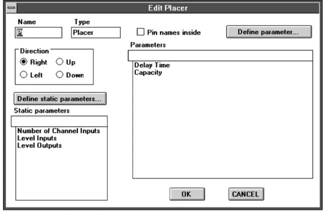
The Placer (its user interface can be seen in
Fig. 4.) is a new basic element of the Petri
Net implementation and it is at the same level as Place or Transition, it behaves in a similar way as the Place element, Placer has a limited capacity as well. This means that the number of tokens in the Placer is restricted, the maximum value of tokens it can contain is its capacity. After a while the tokens can leave the Placer, this time is the total delay time of it. The to-tal delay time can be divided into small delay time increments. The mobile object can move in incremental steps within the total delay time. These incremental steps can be used for visu-alization of moving as opposed to conventional Place element, where the mobile objects remain inside the Place, without indicating its internal movement.
A great advantage of the Placer is its usability in several fields, not only in the railway systems, but in many other systems as e.g. general traffic
systems. So, for example we used Placer ele-ments in simulating urban traffic models(Sz˝ucs
and Benk˝o, 1995; Sz˝ucs et al., 1996; Sz˝ucs et al., 1997).
It is possible to use Placer elements in traffic systems between cities in a country or in a re-gion. Placer element may represent moving airplanes, so any airport can be built by using these objects, where the tokens may represent different types of aircraft. Placer is very use-ful in transport systems and logistic problems, since it helps to solve the problem of conve-nient visualization(Serafeimidis and Smithson,
1996).
6. Simple and Slicing Evade
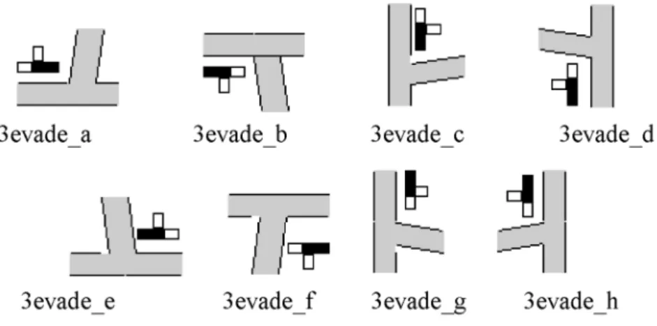
The simple evade(see Fig. 5.) is a branching
part of the railway network, where the trains arriving may prefer a direction. The trains can come into the simple evade from 3 directions and may leave it in 3 directions by observing the following rules: If the train arrives from direction 1, it may leave in direction 2 or direc-tion 3 depending on the posidirec-tion of the switch of the simple evade. The number of the states
Fig. 5.Graphical representation of the simple evades.
Fig. 6.Graphical representation of the slicing evades.
of the switch is 2, because the train must choose between 2 possibilities.
One state is M, meaning that the train must go on the main way, the other is B, in this case the train must choose the byway. If the train comes from direction 2, then it cannot select; the train must leave in direction 1(naturally, the switch
must be in M state avoiding going off). If the
train arrives from direction 3, then it does not have to choose, it will go in direction 1 (the
state of the switch must be B). In our model
the simple evade is operating as a system object with 6 ports, 3 input ports and 3 output ports. The slicing evade (see Fig. 6.) is a complex
branching part of the railroad network, but not only one arriving train can choose an output di-rection. The train arriving at this object from any input direction can choose one way from the existing output directions. The trains can come into the slicing evade from 4 directions and may leave it in 4 directions, as well by observing the following rules:
If the train arrives from any direction, it may leave in two directions, depending on the state of the switch of the evade. The states of the switch are the following, as can be seen in Ta-ble 2.
MS: MainStraight MC: MainCross BS: BywayStraight BC: BywayCross
Arrive Leave State of theswitch From 1 To 2 MS From 1 To 3 MC From 2 To 1 MS From 2 To 4 MC From 3 To 1 BC From 3 To 4 BS From 4 To 2 BS From 4 To 3 BC
7. The Model of the Railway System
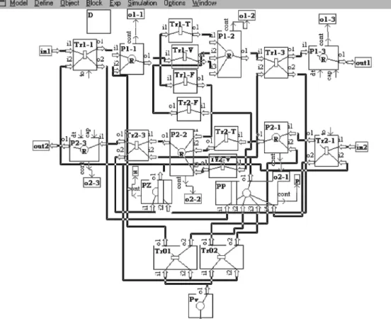
The whole model of the railway system is im-plemented in CASSANDRA using the above described object set. The block of the model of
the full system can be seen in Fig. 7. Since the entire system cannot be seen on one screen, only one railway station can be selected at a time and such a railway station can be seen in the Figure 8.
Fig. 7. Block scheme of the model of the whole system.
8. Schedule and Timetable
The schedule of a train contains all information about the places and the times, when and where the train must be and how much time it has to wait at the railway stations. Scheduling of the whole system consists of the schedules of the trains, but it is a complex task to arrange it so that the trains should not collide and/or wait
too long for each other. The schedule contains time scheduling(timetable)and area scheduling
(route description).
Usually a timetable contains departure times and arrival times at every railway station, where the train stops or passes through without stop-ping. In our simulated model velocity of the trains is determined, so besides the departure times we do not prescribe arrival times, other-wise the system would be overdetermined. Ve-locity of the trains is restricted in two ways. One is the maximum speed of the train, the other is the parameter of each part of the railtrack: re-stricted speed on the given railtrack. The real velocity is calculated from these two velocities, namely the final velocity is the minimum of the maximal train speed and the restricted speed of railtrack.
In our simulation system demons(J´avor, 1992)
control the trains in order to avoid collision. This controlling is similar to a common resource management. If a train enters a critical part of the railway system(as a common resource)
the state of the virtual semaphore correspond-ing to this segment will be changed. The virtual semaphores are system variables in our simula-tion model and these system variables modify the semaphores in the animation of the model at the two end of the railway segment in order to forbid entering in the opposite direction for a train or one following it directly. The animated semaphores will be red. The railway segments are divided into railway tracks, which are the smallest units of the railway system, where only one train can stay. After the train left the first interval, the semaphore after it will be green in order to permit the second train – if any train is waiting for the first train – to enter this segment and follow the first train. Naturally the opposite semaphore is still red.
Creating the timetable is a serious engineering task for experts as well. There are computer
programs for such problems, but they “only” provide the output values, and the end-user does not see the way to the solution. Hence finding appropriate timetable by simulation tools is bet-ter, since the found solution can be visualized on the screen and the user can see the operating of the whole system. The demons with AI(
Win-ston, 1977)can find this solution by changing
the time values of the timetable as model pa-rameters.
Let us see, how can the demon find the optimal timetable by changing a departure time para-meter. The train of identity number 9, at railway station "E" can leave at between 8700 to 9000 of the simulation time. During the search the demon modified the parameter of the 9th train and examined the average delay time of all the trains. Part of the results can be seen in Ta-ble 3, where the first row is the departure time in seconds, the second row is the delay of the 6th train, and the last row is the delay time in seconds.
departure delay aver. delay
8700 163 87.5
8750 163 87.5
8800 163 87.5
8850 163 87.5
8900 170 88.2
8950 220 92.7
9000 270 97.3
Table 3.Results of the search.
The table shows that the best results are be-tween 8700 and 8850, where the 6th train does not have to wait for the 9th train between the station “E” and “D”.
9. Route Description by Knowledge Bases
We use frame type Knowledge Bases (
Rozen-blit and Hu, 1992)for the route description of a
because unnecessary items are eliminated ac-cording to the following rules: In the Knowl-edge Bases it is enough to determine the chosen directions at static objects, where the number of the outputs is more than one, that is, where the mobile object must choose? So we do not need to enumerate all static objects along the route, only the branching objects and the cho-sen direction, and this solution is unambiguous. In our model the Knowledge Bases of the route descriptions of the mobile objects are built ac-cording to these assumptions.
The above described solution is good for such route descriptions, where the mobile objects
(trains)are moving straight between two
branch-ing points and are not turnbranch-ing back on the straight line. If the trains can turn back at cer-tain points, then the route description is more complicated. For this situation we developed a complex solution, where the route description is extended with a turning description as well. The row of the turning is defined in a Knowl-edge Base: at which turning point the train must go on, the Knowledge Base contains G(go on)
character, where the train must turn back, the Knowledge Base contains B (back) character.
So all possibilities of the turning back are deter-mined.
10. Simulation Results
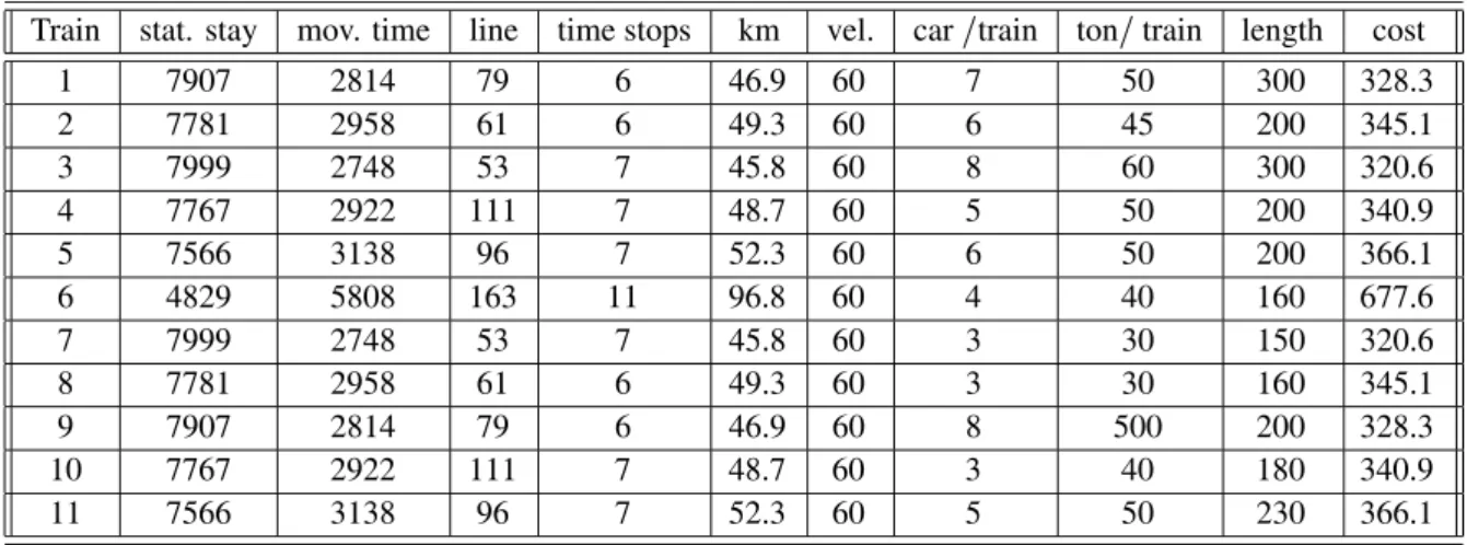
After 3 simulated hours the simulation results of 11 trains can be seen in Table 4.
In the first column the identifier of the train can be found. Stat. staymeans the time of staying on the station,mov. timemeans the moving time andline timeis the time, which the train had to wait on the line between the stations. The next column,stopsshows the number of stoppings,
kmis the whole distance, than the train traveled and thevel. is the velocity of the train.Car/train
shows the number of the cars per train,ton/train
is the weight of the train in tons,length is the length of the whole train with the engine and the cars. The last column shows the cost of the whole round.
11. Summary and Conclusion
Numbers in the table show that the schedule made by railway experts is planned well, be-cause the line time values are small, e.g. the trains did not have to wait long, the maximum of summarized waiting time is less than 3 mi-nutes. This value is at the train, where the trav-eled distance during the simulation is the longest distance. So theline time values are the most important results after the simulation and the students work can be evaluated based on these results. Another important factor is the cost of travelling of the train, which can be used in the economic analysis of the railway system. Operation of the simulation models corresponds to real situations, as various speed limits on the different railroad track segments, halting and waiting of the trains until the continuation of
Train stat. stay mov. time line time stops km vel. car/train ton/train length cost
1 7907 2814 79 6 46.9 60 7 50 300 328.3
2 7781 2958 61 6 49.3 60 6 45 200 345.1
3 7999 2748 53 7 45.8 60 8 60 300 320.6
4 7767 2922 111 7 48.7 60 5 50 200 340.9
5 7566 3138 96 7 52.3 60 6 50 200 366.1
6 4829 5808 163 11 96.8 60 4 40 160 677.6
7 7999 2748 53 7 45.8 60 3 30 150 320.6
8 7781 2958 61 6 49.3 60 3 30 160 345.1
9 7907 2814 79 6 46.9 60 8 500 200 328.3
10 7767 2922 111 7 48.7 60 3 40 180 340.9
11 7566 3138 96 7 52.3 60 5 50 230 366.1
the voyage is permitted(as e.g. one train has to
wait for an other). The appropriate choice of the
level of detail for model representation has been of great importance in order to obtain the rele-vant information from simulation experiments. The simulation supplies a user-friendly graphic model representation with animation giving a good qualitative overview of the system ope-ration, besides providing exact data in form of tables.
As a result of developing an easily modifiable railway system model structure by the AI con-trolled CASSANDRA simulation system, an ef-fective tool to be used both in education and in practical problem solving has been obtained. The simulator has been developed for educa-ting college students and railway operaeduca-ting per-sons, this is more flexible and up to date way than physical railway models. This way, besides training, also experiments for investigating and determining optimal scheduling strategies can be done.
The development for further research may be the investigation of a larger model, in this case the complexity of the system will be greater as well. Such case for example is joining the sub-railway systems (among countries), where the
simulated model is so large, that one computer is not enough for an efficient investigation. The cluster of the workstations may be a good so-lution for these types of problems(Hipper and
Tavangarian, 1998; Shapiro, 1998).
Acknowledgements
This work was undertaken in a project at the Sz´echenyi Istv´an College, when the author was working at the Department of Traffic. Special thanks are due to Professor I. Prileszky, Head of the Department of Transportation for promoting the R&D work. Thanks are also due to Prof. A. J´avor and K. Arat´o for their advice with regard to simulation methodology and railway systems respectively.
References
1] G. HIPPER, D. TAVANGARIAN, A concurrent network
architecture for cost-efficient parallel computing us-ing workstation clusters, Simulation Practice and Theory,6:2(1998), 197–218.
2] A. J ´AVOR, Demon Controlled Simulation,
Mathe-matics and Computers in Simulation, 34:3–4
(1992), 283–296.
3] A. J ´AVOR, Knowledge Attributed Petri Nets,System
Analysis, Modelling, Simulation, 13:1–2 (1993a),
5–12.
4] A. J ´AVOR, Petri Nets in Simulation, EUROSIM
Simulation News Europe, 9 November (1993b),
6–7.
5] A. J ´AVOR, Comparison 2 – CASSANDRA 3.0,
EU-ROSIM Simulation New Europe, 11 July (1994),
28.
6] A. J ´AVOR, G. SZUCS˝ , Traffic Simulation using AI,
presented at the Proceedings of the IMACS Euro-pean Simulation Meeting on Simulation Tools and Applications, 28–30 August,(1995), 76–81, Gyor,˝
Hungary.
7] J. L. PETERSON,Petri Net Theory and Modelling of
Systems, Prentice-Hall, 1981.
8] J. W. ROZENBLIT, J. HU, Integrated knowledge
re-presentation and management in simulation-based design generation,Mathematics and Computers in Simulation,34(1992), 261–282.
9] E. SHAPIRO, Overview New directions for
simula-tion and modeling of complex systems,Simulation Practice and Theory,6:2(1998), 91–97.
10] V. SERAFEIMIDIS, S. SMITHSON, Understanding and
Supporting Information Systems Evaluation, Jour-nal of Computing and Information Technology,4:2
(1996), 121–136.
11] G. SZUCS˝ , M. BENKO˝, An Object Set for Traffic
Simulation, presented at the Proceedings of the IMACS European Simulation Meeting on Simula-tion Tools and ApplicaSimula-tions, 28-30 August,(1995)
82-87. Gyor, Hungary.˝
12] G. SZUCS˝ , ´A. VIGH, A. FARKAS, AI Controlled
Traffic-Emission Line Source,presented at the Pro-ceedings of the ESM96, 2–6 June,(1996)130–134,
Budapest, Hungary.
13] G. SZUCS˝ , A. J´AVOR, M. BENKO˝, GY. BUZASY´ , A.
FARKAS, Traffic Simulation with the AI controlled
CASSANDRA Simulation System, presented at the Proceedings of the 2nd IMACS Symposium on Mathematical Modelling, 5–7 February,(1997)
835–840, Vienna, Austria.
14] G. SZUCS˝ , A. J´AVOR, Simulation and
15] F. TRICAS, J. MARTINEZ, Distributed control systems
simulation using high level Petri nets,Mathematics and Computers in Simulation,46(1998), 47–55.
16] P. H. WINSTON, Artificial Intelligence,
Addison-Wesley Publishing Company, 1977.
Received:May, 2000
Revised:February, 2001
Accepted:May, 2001
Contact address:
G´abor Szucs˝
Department of Information Management Faculty of Economic and Social Sciences Budapest University of Technology and Economics H-1111 Budapest Sztoczek u. 4. HUNGARY e-mail:[email protected]