A Self-Organizing Model for Logic Regression

Vol. 3, No. 2, 2010, 163-173

ISSN 1307-5543 – www.ejpam.com

Email address: [email protected]

http://www.ejpam.com 163 © 2010 EJPAM All rights reserved.

A Self-Organizing Model for Logic Regression

Jerry Farlow

Department of Mathematics, University of Maine, Orono, Maine

__________________________________________________________________________

Abstract: Logic regression, as developed by Ruczinski, Kooperberg, and LeBlanc [1], is a multivariable regression methodology that constructs logical relationships among Boolean predictor variables that best predicts a Boolean dependent variable. More specifically, it finds a regression model of the form

g E Y

[ | ]

= +

b

₀

b L

_{1 1}

+

b L

_{2 2}

+



b L

_{m m} where both the

coefficients

b b

₀

, ,...,

₁

b

_m and the logical expressionsL_j, j=1,...,m are determined, whereby a logical expression one means logical relationships among the predictor variables, such as

1 2

"

X X

,

are true but not

X

₅

"

, or

"

X

₃

,

X

₅

,

X

₇ are true but not

X

₁ or

X

₂

"

In paper [1] the authors investigate the use a simulated annealing algorithm. In this paper. the Group Method of Data Handling (GMDH) is used.

2000 Mathematics Subject Classifications: 62

Key Words and Phrases: Logic regression, GMDH, algorithm, self-organizing methods.

__________________________________________________________________________ 1. Introduction

In this paper we study the possibility of using Ivakhenko’s Group Method of Data Handling (GMDH) algorithm for finding the best logical expressionsL_j among Boolean

predictor variables

X X

₁

,

₂

,



,

X

_m which best predicts a dependent Boolean variable Y. By logical expressionsL_j, we mean Boolean expressions such as

"

X X

₁

,

₂ are true but not

X

₅

"

2. Basic Group Method of Data Handling (GMDH) Algorithm 2.1 Basic GMDH Method

If one were to anthropomorphize, one might say the GMDH algorithm builds a mathematical model similar to the way biological organisms are created through evolution. That is, starting with a few basic primeval forms (i.e. equations); one grows a new generation of more complex off-springs (equations) and then allows for a survival-of-the-fittest principle to determine which new off-springs survive and which do not. The idea is that new generations of off-springs (equations) are better suited to model the real world than earlier ones. Continuing this process for more generations, one finds a collection of models that hopefully describes the problem at hand. The process is stopped once the model begins to “over-fit” the real world, thus stopping when the model reaches some level of optimal complexity.

In 1966, Ukrainian cyberneticist, A.G. Ivakhnenko, discouraged by the fact that many mathematical models require the modeler to know things about the real world that are difficult or impossible to know, produced a heuristic self-organizing model, called the Group Method of Data Handling algorithm. For more information see Farlow, [1] or view one of the many websites which discuss applications of the technique. Ivakhnenko’s website at

The basic GMDH algorithm can be broken into a few distinct steps.

Step 1 (constructing new variables z z₁, ₂,...,z_{C m( ,2)})

The basic GMDH algorithm begins with regression-type data points of the form

1 2 1 2

, , ,..., , , ,...,

i i i im

y x x x i= n, where the

n

observations are subdivided into two groups,

the first

nt

observations are called the training observations and the remaining

nc

= −

n nt

observations are called the checking observations. See the data in Figure 1. Normally, about half the observations are chosen to be in each group.

Y X

Training set

Y

x

₁

x

₂ 

x

m

1

y

x

₁₁

x

₁₂ 

x

1m

2

y

x

₂₁

x

₂₂ 

x

2m

    

nt

y

xnt,1 xnt,2  xnt m,

Checking set

1

nt

y

₊ xnt+1,1 xnt+1,2  xnt+1,m

    

n

y

xn,1 xn,2 

x

nm

Now, for each

C m

( , 2)

=

m m

(

−

1) / 2

pair of distinct variablesx x_i, _j one finds the least-squares regression polynomial for y of the form

2 2

i j i j i j

y= +A Bx +Cx +Dx +Ex +Fx x (1)

(i.e. find

A B C D E F

, , , , ,

) from the observations in the training set These

m m

(

−

1) / 2

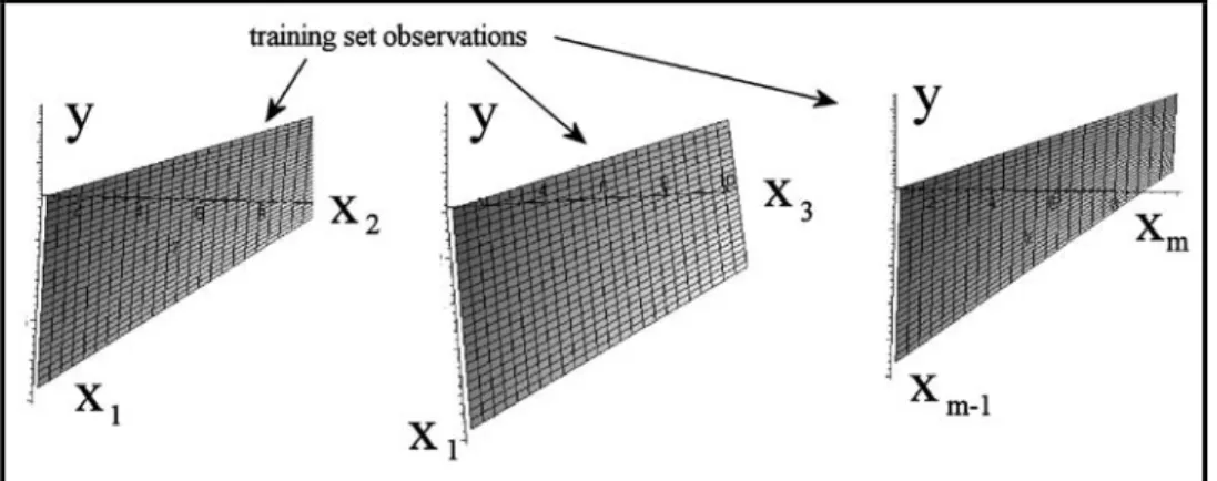
regression surfaces are illustrated in Figure 2.

Figure 2: Computed Quadratic Regression Surfaces

Now evaluate each of the

m m

(

−

1) / 2

regression polynomials at all n data points and store these values (new generation of variables) in the respective columns of a new array, say Z. The evaluation of the first regression polynomial and its values in the first column of Z is illustrated in Figure 3.

The object is to keep only the best of these new variables and this is where the observations in the checking set come into play.

Step 2 (screening out the least effective variables)

This step replaces the original variables (columns of X) by those columns of Z that best predict y, based on the checking set observations. That is, for each column j of Z we compute the root mean square (or some measure of association)

r

_j given by Eq. (2).

2

2 1

2

1

(

)

,

1, 2,..., ( , 2)

n

i ij i nt

j n

i i nt

y

z

r

j

C m

y

= +

= +

−

=

∑

=

∑

(2)

and then select those columns of Z that satisfy rj <R, where R is some prescribed number. The number of columns of Z that replace columns of X may be larger or smaller than the number of columns of X, although often one keeps the number of columns of X constant at m. Note that the test of goodness of fit r_jwas summed over the observation in the checking set.

Step 3 (test for optimality)

From Step 2 we find the smallest of the r sj' and call it RMIN. Then, each time one

completes a generation or iteration, one plots the value of RMIN on a graph as shown in Figure 4.

Experiments have shown that RMIN decreases for a few generations (the author’s experience is maybe 3-5 iterations) and then begins to increase, the reason being the model gets better and better but eventually starts to over-fit the data. Hence, the rule is to stop the algorithm when the RMIN curve reaches its minimum, and then select the column with the minimum r_j value of the final array Z as the best predictor. When the GMDH algorithm

stops, the columns of Z (in particular the column of Z that has the smallest r_j value) contains the computed values of a high-order polynomial of the form in Eq (3)

1

1 1 1 1 1 1

m m m m m m

i i ij j j ijk i j k

i i j i j k

y

a

b x

c x x

d x x x

= = = = = =

= +

∑

+

∑∑

+

∑∑∑

+



(3)

known as the Ivakhnenko polynomial. At each iteration the degree of the Ivakhnenko doubles, and for a p-th order regression polynomial the number of terms in the polynomial will be

(

m

+

1)(

m

+

2)



(

m

+

p

) /

m

!

. For example, if one starts with m=10 input variables

x x

₁

,

₂

,...,

x

₁₀ and the algorithm is continued for 8 generations, the Ivakhnenko

polynomial would be a polynomial in

x x

₁

, ,...,

₂

x

_m of degree

2

8

=

256

. A sample term

might involve the variables x x x x x x₁2 ₃4 ₄9 ₆11 ₇9 ₁₀3 .

Step 4 (Applying the results of the GMDH Algorithm)

One doesn’t actually compute the coefficients in the Ivakhenko polynomial, but saves the regression coefficients A,B,C,D,E,F at each generation. Hence, to evaluate the Ivakhnenko polynomial one simply carries out repeated compositions of these quadratic expressions. Figure 5 illustrates this process.

3. GMDH Algorithm Applied to Logic Regression Step 1: (Divide Observations into Training and Checking Sets)

Starting with n observations of m Boolean predictor variables

X X

₁

,

₂

,...,

X

_mand a dependent Boolean variable Y, we subdivide the observations into nt training set observations and

nc

= −

n nt

checking set observations. For each of the

(

1)

2

2

m

m m

 

₌

−

 

 

distinct pairs

{

X X

i

,

j

:

i

=

1,..

m

−

1,

j

= +

i

1,

m

}

of predictor variables, we find the logical function that best predicts the dependent variable

Y

from among the 16 binary functions in Table 1.

Table 1: Sixteen Boolean Functions

0(0000) FFFF never true ---

1(0001) FFFT _{not (}

1

X

or

X

₂)

X

₁

∧

X

₂ 2(0010) FFTF

2

X

but not

X

₁ X₁∧X₂

3(0011) FFTT _not

1

X

X₁

4(0100) FTFF

1

X

but not

X

₂ X₁∧X₂

5(0101) FTFT _not

2

X

X₂

6(0110) FTTF

1

X

or

X

₂ but not both

X

₁

∨

X

₂ 7(0111) FTTT _{not (}

1

X

and

X

₂) X₁∨X₂

8(1000) TFFF

1

X

and

X

₂

X

₁

∧

X

₂ 9(1001) TFFT

1

X

is

X

₂

X

₁

≡

X

₂

10(1010) TFTF

2

X

X

₂

11(1011) TFTT _If

1

X

then

X

₂

X

₁

⇒

X

₂ 12(1100) TTFF

1

X

X

₁

13(1101) TTFT _if

2

X

then

X

₁

X

₁

⇐

X

₂

14(1110) TTTF

1

X

or

X

₂

X

₁

∨

X

₂

16(1111) TTTT always true ---

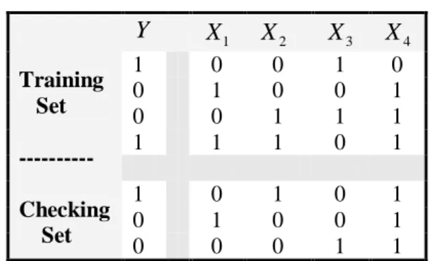
We illustrate the process with the data set in Table 2, which has n=7 _{total observations,} 4

Table 2: Sample Data Training Set --- Checking Set

Y

X

₁

X

₂

X

₃

X

₄

1 0 0 1 0

0 1 0 0 1

0 0 1 1 1

1 1 1 0 1

1 0 1 0 1

0 1 0 0 1

0 0 0 1 1

Note that the dependent variable

X

₁ did not predict Y in the first- and second observations (1s and 0s do not match), but do predict Y in the 3rd and 4th observations (1s and 0s match). Note, too that the logical relation X₁∧X₂ correctly predicts Yin the 1st, 2nd, and 3rd observations, but not the 4th, hence the recorded values 1, 1, 1, and 0 in the respective column, and a 3 in the bottom row illustrating the number of correct predictions. If one carries out this analysis for all 16 logical expressions of

X X

₁

,

₂, one arrives at the results in Table 3.

Table 3: Correct and Incorrect Predictions of Yfrom

X X

₁

,

₂.

0 (0000) false

1 (0001)

1 2

X ∧X

2 (0010)

1 2

X ∧X

3 (0011)

1 X

4 (0100)

1 2

X ∧X

5 (0101)

2 X

6 (0110)

1 2

X

∨



X

7 (0111)

1 2

X ∨X

0 1 0 1 0 1 0 1

1 1 1 1 0 0 0 0

1 1 0 0 1 1 0 0

0 0 0 0 0 0 0 0

2 3 1 2 1 2 0 1

8(1000)

1 2

X

∧

X

9(1001)

1 2

X

≡

X

10(1010)

2

X

11(1011)

1 2

X

⇒

X

12(1100)

1

X

13(1101)

1 2

X

⇐

X

14(1110)

1 2

X

∨

X

15(1111) tautology

0 1 0 1 0 1 0 1

1 1 1 1 0 0 0 0

1 1 0 0 1 1 0 0

1 1 1 1 1 1 1 1

3 4 2 3 2 3 1 2

Note the best logical predictor is 9(1001), which represents the logical function

X

₁

≡

X

₂.

variables, and the bottom row 3 gives the fraction (and percentage) of times the given logical function accurately predicted Y.

Table 4: Results for the first iteration.

Variable

pairs

X X

1

,

2

X X

1

,

3

X X

1

,

4

X

2

,

X

3

X

2

,

X

4

X

3

,

X

4

Function X1 ≡X2

X

1

∧

X

3

X

1

∨

X

4

X

2

⇐

X

3

X

2

⇒

X

4 X3∨X4

# correct 4/4(100%) 3/4(75%) 4/4(100%) 2/4(50%) 3/4(75%) 2/4 (50%)

The next step is to select the best

m

functions from Table 4 (4 in this example) that predictsY.

Step 2: (Replace the Original Data with the Best Logical Estimates)

We now evaluate the best

m

logical functions in Table 4, which represent the best logical predictors of Ybased on the observations in the training set. In this example they are

1 2

X

≡

X

,

X

₁

∧

X

₃,

X

₁

∨

X

₄,

X

₂

⇒

X

₄ which yields 4, 3, 4, and 3 correct predictions. Evaluating these functions at the

n

observations, we arrive at the

n m

× = ×

4 4

array in Table 5, which we call XNEW and are the evaluated best predictors of Y. Note that in the column under

X

₂

⇒

X

₄ for the observations in the checking set, the values are 1, 1, and 1, which are the logical evaluations of the corresponding observations in the original data matrix X in Table 2. We now replace the data matrix X of independent variables with the newly computed matrix XNEW.

Table 5: New Computed Data XNEW Replaces X.

Training Set

---

Checking Set

1 2

X

≡

X

X

1

∧

X

3

X

1

∨

X

4

X

2

⇒

X

4

1 0 1 0 0 0 0 1 0 1 1 1 1 1 0 1

1 0 0 1

0 0 1 1

0 0 0 1

Step 3: (When to Stop: Goodness of Fit)

stops, the columns of XNEW contain the computed values of the best

m

logical predictors of

Y. This defines the algorithm.

4. Computations

We tested the algorithm’s ability to find best logical relations of several independent variables from among m=50 independent variables with n=250 observations (nt=150,nc=100). All independent variables were binary 0 and 1 variables, each having probability 0.5. The dependent variable Ywas generated as a logical expression of the dependent variables for some observations, and random 0s and 1s for other observations. In this way we could determine how well the GMDH algorithm works.

To carry out the generation of the dependent variable Y, we first select a number

0

≤ ≤

q

1

, then generate a uniform random number

r

between 0 and 1, and then the observations

y i

i

,

=

1,...,

n

computed by the rule

specified logical function when

random 0 or 1 when

i

r q

y

r

q

≥



= 

_<



Note that when

q

=

0

the dependent observations

y

_i are the values of specified logical

function of the dependent variables, and when

q

=

1

the computed values of

Y

are random 0s and 1s and have no relation to the independent variables. The goal was to determine how well the algorithm could pick out the chosen logical relation when

0

< <

q

1

.

Experiment 1: The value

q

=

1

was chosen with logical function

X

₁₅

⇒

X

₃₅. It was not surprising that at the first iteration the maximum logical function was

X

₁₅

⇒

X

₃₅ and that it predicted the dependent variable 150 out of 150 times in the training set and 100 out of 100 times in the checking set. The second through fifth place logical relations were (2)

15 42

X

⇒

X

, (3) not both X₁₅ and X₄₉, (4)

not both

X

₁₅

and

X

₁₆, and (5)

X

₁₆

⇒

X

₃₅ which is not surprising since the chosen logical relation X₁₅⇒ X₃₅ ≡ X₁₅∪X₃₅ so the variables

15 and 35

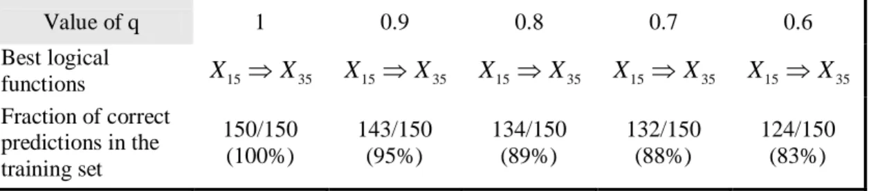
X X would naturally come into play. The following Table 6 shows the results for the same logical function for different values of q after 1 iteration.

Table 6: Correct predictions of Yafter 1 iteration for different values of q.

Value of q 1 0.9 0.8 0.7 0.6

Best logical

functions

X

15

⇒

X

35

X

15

⇒

X

35

X

15

⇒

X

35

X

15

⇒

X

35

X

15

⇒

X

35

Fraction of correct predictions in the training set

150/150 (100%)

143/150 (95%)

134/150 (89%)

132/150 (88%)

Fraction of correct predictions in the checking set

100/100 (100%)

97/100 (97%)

89/100 (89%)

84/100 (84%)

79/100 (79%)

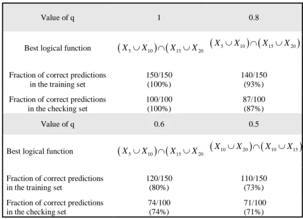
Experiment 2: Using the same data and values of q as in Experiment 1, but with the new logical function y=

(

X₅∪X₁₀

) (

∩ X₁₅∪X₂₀

)

, we arrived at the results in Table 7 after two iterations. In these cases the algorithm reached its maximum predictions after only two iterations. Note that when

q

=

0.5

the maximum logical function was close to the entered logical function but not exact. This is not surprising since only 50% of the dependent variables were computed from y_i =

(

X₅∪X₁₀

) (

∩ X₁₅∪X₂₀

)

.

Table 7: Results after 2 Iterations

Value of q 1 0.8

Best logical function

(

X₅∪X₁₀

) (

∩ X₁₅∪X₂₀

)

(

X5∪X10

) (

∩ X15∪X20

)

Fraction of correct predictions in the training set

150/150 (100%)

140/150 (93%)

Fraction of correct predictions in the checking set

100/100 (100%)

87/100 (87%)

Value of q 0.6 0.5

Best logical function

(

X₅∪X₁₀

) (

∩ X₁₅∪X₂₀

)

(

X10∪X20

) (

∩ X10∪X15

)

Fraction of correct predictions in the training set

120/150 (80%)

110/150 (73%)

Fraction of correct predictions in the checking set

74/100 (74%)

71/100 (71%)

5. Conclusions

References

[1] I. Ruczinski, C. Kooperberg, and M. LeBlanc. Logic Regression. Journal of Computational and Graphical Statistics 12(3), 475-511, 2003.