CONFORMAL PERTURBATIONS AND LOCAL SMOOTHING
Dylan Muckerman
A dissertation submitted to the faculty at the University of North Carolina at Chapel Hill in partial fulfillment of the requirements for the degree of Doctor of Philosophy in the
Department of Mathematics in the College of Arts and Sciences.
Chapel Hill 2018
ABSTRACT
Dylan Muckerman: Conformal Perturbations and Local Smoothing (Under the direction of Hans Christianson)
The purpose of this paper is to study the effect of conformal perturbations on the local smoothing effect for the Schr¨odinger equation on surfaces of revolution. The paper [CW13] studied the Schr¨odinger equation on surfaces of revolution with one trapped orbit. The dynamics near this trapping were unstable, but degenerately so. Beginning from the metric
TABLE OF CONTENTS
CHAPTER 1: INTRODUCTION . . . 1
CHAPTER 2: BACKGROUND . . . 3
2.1 Schr¨odinger equation . . . 3
2.1.1 Notations and Conventions . . . 6
2.2 Pseudodifferential Operators . . . 6
2.2.1 Basic definitions . . . 6
2.2.2 Symbol calculus . . . 7
CHAPTER 3: LOCAL SMOOTHING IN EUCLIDEAN SPACE . . . 10
3.1 Background and motivation . . . 10
3.2 Positive Commutator argument . . . 12
CHAPTER 4: LOCAL SMOOTHING IN THE PRESENCE OF TRAPPING 16 4.1 Necessity of a Loss . . . 17
4.2 Surfaces of Revolution . . . 18
CHAPTER 5: CONFORMAL PERTURBATIONS OF SURFACES OF REV-OLUTION . . . 21
5.1 Positive Commutator . . . 25
5.2 Estimating in the Frequency Domain . . . 33
5.3 High Frequency Estimate . . . 42
5.4 Microlocal proof of the Resolvent Estimate . . . 44
CHAPTER 1 Introduction
In this thesis we discuss the effect of conformal perturbtions on local smoothing of the Schr¨odinger equation on surfaces of revolution.
The local smoothing effect was introduced and first studied for the Korteweg-de Vries equation in [Kat83]. It was studied for the Schr¨odinger equation in the papers [CS88], [Sj¨o87], [Veg88], and [KY89]. In [Sj¨o87] and [Veg88], it was used to prove almost everywhere pointwise convergence of solutions to the Schr¨odinger equation to their initial data as t→0.
The paper of [Doi96] showed the connection between the local smoothing effect and the geometry of the underlying manifold, by showing that the full local smoothing effect of 1/2 of a derivative holds if and only if the manifold has no trapped sets.
Following this were a number of results on local smoothing in the presence of trapped sets, including [Bur04], [Chr07], [Chr08], [Chr11], [Dat09], [CW13], [CM14], and [Chrar]. In these papers it was shown that while the full local smoothing effect of 1/2 does not hold, there are many conditions under which a smaller degree of local smoothing does hold. Very broadly speaking, the less stable the trapping, the greater the degree of local smoothing.
In particular, the results in [CW13] and [CM14] concern the degree to which the local smoothing effect for the Schr¨odinger equation holds on a surface of revolution with a finite number of trapped orbits for which the dynamics near the trapped set are unstable, but degenerately so. Because of this degeneracy, the trapping is not stable under conformal perturbations. Hence there is a possibility of changes in the trapped set and therefore the local smoothing.
the unperturbed manifold.
We begin by giving some background on the Schr¨odinger equation and pseudodifferential operators. In particular, we develop a pseudodifferential calculus suited to our needs. This calculus can be thought of as a hybrid of the classical and semiclassical calculuses.
We then give an overview of local smoothing in Euclidean space. Particular attention is given to using a positive commutator argument to prove local smoothing. This argument will form the initial basis for our main proof.
After that we turn to local smoothing in the presence of trapping. We state the results here in some detail, as our result is concerned with a very similar setting.
We finally give the statement and proof of our main result. The proof works by emulating the proofs in [CW13] and [CM14], though it should be noted that the reduction to one dimension used in those papers is no longer available to us. In proving the local smoothing estimate away from the region of the trapping on the unperturbed manifold, we are able to emulate the previous proofs very closely, using the positive commutator argument. This is also the case in the positive commutator argument used to reduce the proof to a microlocal resolvent estimate.
CHAPTER 2 Background
2.1 Schr¨odinger equation
Let M be a Riemannian manifold with metric g and Laplace-Beltrami operator ∆g. Let
Dt denote 1i∂t. The Schr¨odinger equation is
(Dt−∆g)u= 0
u|t=0 =u0.
A very important property of solutions to the Schr¨odinger equation is that they have constant
L2 norm. We prove this in Euclidean space for u0 in the Schwartz class of functions
S(Rn) ={f ∈C∞
(Rn) : |xα∂βf| ≤Mαβ}.
That is, f and all of its derivatives decay more quickly than any polynomial.
We can write the solution u explicitly using the Fourier transform. Let ˆu(ξ, t) denote the Fourier transform in x of u(x, t). Then
ˆ
u=ei|ξ|2tuˆ0.
Schwartz class is preserved by the Fourier transform, hence ˆu0 ∈ S. Furthermore, for every t, ei|ξ|2t
and all of its derivatives inξ grow at most polynomially. Therefore ˆu∈ S and hence
We begin by letting
E(t) =kuk2
L2 and calculating
E0(t) = Z
Rn
(∂tu)u+u(∂tu)dx = Re
Z
Rn
(∂tu)u dx.
We then use the fact that usolves the Schr¨odinger equation to conclude that this equals
E0(t) = Re Z
Rn
i∆(u)u dx
= Re−i
Z
Rn
|∇u|2dx
= 0,
where we have also made use of integration by parts. This proves that E(t) =E(0) as long as u0 (and hence u) is in S. Using the fact that S is dense in L2 then allows us to extend
this argument to all of L2.
This result can be strengthened to show that all of the Hs Sobolev norms are constant for solutions to the Schr¨odinger equation. We introduce the useful notation
hξi= (1 +ξ2)1/2
and let
Λsu=F−1(hξisuˆ),
transform. Recall that the Hs norms are defined as
kukHs =kΛsukL2.
Let eit∆ denote the Schr¨odinger propagator, which we define using the Fourier transform, by
eit∆u=F−1eit|ξ|2 ˆ
u.
We need to commute the operators Λs and eit∆. To see that they commute we note that
both Λs and eit∆ are both Fourier multipliers and hence
Λseit∆u=F−1hξisFF−1eit|ξ|2uˆ
=F−1hξis
eit|ξ|2uˆ =F−1eit|ξ|2
hξisuˆ =F−1eit|ξ|2
F F−1(hξis ˆ
u) =eit∆Λsu.
We can then combine this with the earlier conservation of L2 norm to find
kukHs =kΛseit∆u0kL2 =keit∆(Λsu0)kL2 =kΛsu
0kL2 =ku0kHs,
2.1.1 Notations and Conventions
We will use C to denote a large constant which may change from line to line. We will similarly use c to denote a small positive constant which may change from line to line.
2.2 Pseudodifferential Operators
Our outline of pseudodifferential operators will follow the presentation of [Zwo12], [Tay81], and [Tay13].
2.2.1 Basic definitions
In the above definition of Sobolev spaces, we made use of an operator defined by multipli-cation conjugated by the Fourier transform. Writing this out explicitly, we find
Λsu(x) = 1 (2π)n
Z Z
eihx−y,ξihξisu(y)dydξ.
Replacing the function hξis with a more general function leads to a very useful class of operators.
We will work with the symbol classes Sm
ρ , ρ≥0 originally defined in [H¨or66], given by
Sρm ={a∈C∞(R×R×S1×Z) : |∂ξα∂xβ∂θγ∂ηδa| ≤Cα,β,δ,γhξi m−|α|ρ
hηi−|δ|ρ},
where ∂η denotes a difference operator in η. In particular, we will work with a symbol supported only where |ξ| ≤C|η|, allowing us to transfer decay in |η| to decay in |ξ|.
Define
awu= 1 (2π)2
Z
R2
Z S1
X η
eihx−x,ξ˜ i+ihθ−θ,η˜ ia x+ ˜x
2 ,
θ+ ˜θ
2 , ξ, η !
u(˜x,θ˜)dθd˜ xdξ˜
of a. It should be noted that the Weyl quantization is just one choice of many quantizations. The function a is said to be the symbol of the operator.
2.2.2 Symbol calculus
We review a few essential theorems of the symbol calculus.
Theorem 2.2.1 (Calderon-Vaillancourt Theorem). If a∈S0
0 then the operator aw is bounded
as an operator from L2 to L2.
This theorem is originally due to [CV71]. See Theorem 4.23 in [Zwo12] for another proof. In fact, a more general theorem holds.
Theorem 2.2.2. If a∈Sm
0 then the operatoraw(x, D) is bounded as an operator fromHs+m
to Hs.
Quantization does not commute with composition. That is to say, the composition of two pseudodifferential operators is not the quantization of the product of their symbols. In fact, it is not immediately obvious that the composition of two pseudodifferential operators is a pseudodifferential operator. In fact, the following theorem holds.
Theorem 2.2.3 (Theorem 4.18 in [Zwo12]). Let a∈Sm
ρ , b ∈Sρm˜. Let
A(D) = 1
2(hDξ, Dyi − hDx, Dηi).
Then
aw(x, D)◦bw(x, D) =cw(x, D)
for
c=a#b := N X
k=0 ik k!A(D)
k
a(x, ξ)b(y, η)
x=y,ξ=η +r,
In particular,
Corollary 2.2.4. Let a∈Sm
ρ , b ∈Sρm˜. Then
a#b=ab+ 1
2i{a, b}+r,
where r ∈Sm+ ˜m−2ρ
ρ .
This can be seen from the symbol expansion for the commutator of aw and bw using Theorem 2.2.3. Due to the symmetry of the Weyl quantization, the following holds.
Corollary 2.2.5. Let a∈Sm
ρ , b ∈Sρm˜. Then the commutator
[aw(x, D), bw(x, D)] =cw(x, D),
where
c= 1
i{a, b}+r,
and r∈Sρm+ ˜m−3ρ.
Note that we gain 3 in the symbol class of the remainder term, rather than the gain of 2 we may naively expect. See Theorem 4.12 in [Zwo12].
Another useful feature of the Weyl quantization is the following theorem.
Theorem 2.2.6. Let a be a real symbol. Then the operator aw is essentially self-adjoint. A final result we require is the G˚arding inequality.
Theorem 2.2.7. Let a∈Sm
ρ with 0≤ρ≤1 and suppose
Rea≥C|(ξ, η)|m
for |(ξ, η)| large. Then for any s∈R there exist C1, C2 such that for all u∈Hm/2,
Rehawu, ui ≥C1kuk2Hm/2 −C2kuk
2
CHAPTER 3
Local smoothing in Euclidean space
3.1 Background and motivation
In Euclidean space, the local smoothing result for the Schr¨odinger equation states that on average in time, and locally in space, solutions to the Schr¨odinger equation gain half a derivative compared to their initial data. More precisely, for everyT > 0 there exists CT >0 such that if u solves
(Dt−∆)u= 0
u|t=0 =u0,
then
Z T
0
k hri−3/2∂ruk2+k hri
−1/2
r−1∇Sn−1uk2dt≤CTku0k2 H1/2, for all u0 ∈H1/2. Note that the spatial weights are not sharp.
Local smoothing for the linear Schr¨odinger equation was first studied by [CS88], [Sj¨o87], [Veg88], and [KY89]. Both [Sj¨o87] and [Veg88] made use of this inequality to prove that solutions of the Schr¨odinger equation converge pointwise almost everywhere to their initial data as t→0.
We give a simple proof of this result, similar to those in [Tao06] and [CW13]. As in our above statement of the theorem, we make use of polar coodinates. We begin with a simplified version of the argument which does not quite work. In seeing where it fails, we see the appropriate properties the commutant should have.
Recall that r∂r =x·∂x. Then
[r∂r,∆] = [x1∂x1 +. . .+xn∂xn, ∂
2
x1 +. . .+∂
2
Most of the terms in this commutator vanish, as
[xk∂xk, ∂
2
xj] = 0
for j 6=k. Thus
[r∂r,∆] = n X
k=1
[xk∂xk, ∂
2
xk]
= n X
k=1
xk(∂x3k)−∂
2
xk(xk∂xk)
= n X
k=1
xk∂x3k −∂xk(∂xk +xk∂
2
xk)
= n X
k=1
xk∂x3k −2∂
2
xk +xk∂
3
xk
=−2∆.
In order to make use of integration by parts, we will assume u∈ S. The result can then be concluded for all u∈H1/2 using a density argument. We have
0 = Z T
0
hr∂r(Dt−∆)u, ui − hr∂ru,(Dt−∆)ui dt
= Z T
0
h[r∂r,−∆]u, ui dt+ihr∂ru, ui| T t=0.
Rearranging and using the computation of the commutator from above, we find
Z T
0
h−∆u, ui dt≤
hr∂ru, ui| T t=0
.
The left hand side is
Z T
0
kuk2 ˙
H1dt,
would be to average the derivative over the inner product and bound the entire inner product by kuk2
H1/2 evaluated at t= 0 andt =T. We would then use the fact that the H
˜
s norms are bounded for the Schr¨odinger equation: There exists C >0 such that
kukHs˜ ≤Cku0kHs˜.
We would then conclude an upper bound ofku0k2H1/2. The problem is thatr is not a bounded operator on Hs˜.
3.2 Positive Commutator argument
To fix this argument, we replace the unbounded commutantr∂rwith the boundedhri
−1 r∂r. Near 0 this is approximately the same as our earlier commutant, so we expect that this should recover the same result near 0. We need to compute [hri−1r∂r,∆]. We do this in a few pieces. First
[hri−1r∂r, ∂r2] =hri
−1
r∂r3−∂r2(hri−1r∂r)
=hri−1r∂r3−∂r2(hri−1r)∂r−2∂r(hri
−1
r)∂r2− hri−1r∂r3
=−∂r(hri
−3
)∂r−2hri
−3 ∂r2
= 3rhri−5∂r−2hri
−3 ∂r2.
Next
hri−1r∂r,
n−1
r ∂r
= (n−1)
(hri−1r∂r)( 1
r∂r)−
1
r∂r(hri
−1 r∂r)
= (n−1)
− hri−1r−1+hri−1∂r2− 1
r hri
−3
∂r− hri
−1 ∂r2
= (n−1)− hri−1r−1(1 +hri−2)∂r
Finally,
[hri−1r∂r, r−2∆Sn−1] =hri−1r∂r(r−2∆Sn−1),−r−2∆Sn−1(hri−1r∂r) =−2hri−1r−2∆Sn−1.
So we find
0 = Z T
0
hri−1r∂r(Dt−∆)u, u
−
hri−1r∂ru,(Dt−∆)u dt = Z T 0
[hri−1r∂r,−∆)u], u
dt+i
hri−1r∂ru, u
T t=0.
We arrange this and use our computation of the commutator to find
Z T
0
3rhri−5∂r−2hri
−3
∂r2u, u
+ (n−1)− hri−1r−1(1 +hri−2)∂r
−2hri−1r−2∆Sn−1u, u
dt
≤
hri−1r∂ru, u T t=0 .
We work first on the upper bound. We have
hri−1r∂ru, u = D
hDri
−1/2
hri−1r∂ru,hDri
1/2 uE
≤ k hDri
−1/2h
ri−1r∂rukL2k hDri1/2ukL2.
We immediately have k hDri
1/2
ukL2 ≤CkukH1/2. The other term can be bound by consider-ation of symbol classes. The symbolhri−1r is bounded, as are all of its derivatives, so it’s in
this composition is bounded as an operator from H1/2 to L2, so
k hDri
−1/2
hri−1r∂rukL2 ≤ kukH1/2.
We have thus shown that
hri−1r∂ru, u T t=0
≤ kuk
2
H1/2
t=0
+kuk2
H1/2
t=T
.
Because u solves the Schr¨odinger equation, it has Hr norm controlled by the Hr norm of the initial data and thus
hri−1r∂ru, u T t=0
≤Cku0k
2
H1/2. Next we will work on the lower bound. The easiest part is
Z T
0
−2hri−1r−2∆Sn−1u, u
dt = Z T
0
2k hri−1/2r−1∇Sn−1uk2dt.
Next we have
Z T
0
−2hri−3∂r2u, u dt= 2 Z T
0
∂ru, ∂r(hri
−3
u) dt
= 2 Z T
0
∂ru,hri
−3 ∂ru
+∂ru,(−3)rhri
−5
u, u dt
= Z T
0
2k hri−3/2∂ruk2dt+
∂ru,(−3)rhri
−5
u, u dt.
over both sides of the inner product: Z T 0
3rhri−5∂ru, u dt = Z T 0 D hDri
−1/2
3rhri−5∂ru,hDri
1/2 uE dt
≤ Z T 0
k hDri
−1/2
3rhri−5∂rukk hDri
1/2 ukdt
≤C
Z T
0
kuk2
H1/2dt ≤C
Z T
0
ku0k2H1/2dt ≤CTku0k2H1/2.
Next we have
Z T 0
− hri−1r−1(1 +hri−2)∂ru, u dt = Z T 0 D hDri
−1/2 − h
ri−1r−1(1 +hri−2)∂ru
,hDri1/2u E dt ≤C Z T 0
kuk2
H1/2dt ≤CTku0kH1/2.
In the two preceding strings of inequalities we have made use of the pseudodifferential calculus to bound the terms involving hDri−1/2, just as we did in proving the initial upper bound. All together, this gives the following local smoothing inequality:
Z T
0
k hri−3/2∂ruk2+k hri
−1/2
CHAPTER 4
Local smoothing in the presence of trapping
One perspective on the local smoothing effect is that it arises from the dispersive nature of the Schr¨odinger equation. In particular, high frequency parts of solutions to the Schr¨odinger equation have higher velocity. By looking locally at solutions, we see “less” of the high frequency part of our solution, and this is what is responsible for the local smoothing. In other words, the high frequency parts of the solution go off to infinity very quickly. In Euclidean space, where the geodesics are straight lines, this is very easy to visualize, and the above result makes it rigorous. On the opposite extreme, we can consider the Schr¨odinger equation on the simplest compact manifold, S1.
Let k ∈Z and consider the function ek(θ) = eikθ. Because
∂θ2ek =−k2ek,
this is an eigenfunction with eigenvalue −k2. Let
uk =e−itk 2
ek(θ).
Then
Dtuk =−k2e−itk 2
ek(θ) =eitk∆ek(θ) = ∆uk,
and hence uk is a solution to the Schr¨odinger equation with initial dataek(x).
Conveniently, ek(θ) is already written as a Fourier series, where the k-th coefficient is 1 and all other coefficients are 0. We compute
Letg be a smooth, non-vanishing function. Then
kgukkH1 ≥ k∂θ(guk)kL2
≥ kg∂θukkL2 − k(∂θg)ukkL2.
Because u is smooth and S1 is compact, we know
k(∂θg)ukkL2 ≤max(∂θg)≤Cg.
On the other hand since g is non-vanishing,
kg∂θukkL2 ≥min|g|k∂θukkL2 = (min|g|)k.
By taking k large enough we can ensure
kgukkH1 ≥Ck
for someC which may be ong. Thus, for r <1, there is no hope of achieving a bound of the form
Z T
0
kgukk2H1dt≤Ckekk2Hr
for all k.
This agrees with our heuristic argument: The high frequency parts of the solution cannot escape to infinity, so they continue to contribute to theHr norms.
4.1 Necessity of a Loss
complete geodesic that remains in a compact set for all time.
The relationship between trapping and local smoothing was explored in [Doi96]: On asymptotically Euclidean manifolds, solutions to the Schr¨odinger equation exhibit 1/2 of a derivative of local smoothing if and only if the manifold has no trapped geodesics.
The next question which arises is to what degree the local smoothing effect still holds when a trapped set exists.
The results in [Bur04], [Chr07], [Chr08], [Chr11], and [Dat09] showed that in the presence of non-degenerate hyperbolic trapping, for any > 0, there is local smoothing of 1/2−
derivatives for the Schr¨odinger equation.
4.2 Surfaces of Revolution
In [CW13], local smoothing is studied on surfaces of revolution that have periodic geodesics which are unstable, but degenerately so. In other words, the curvature vanishes to degree 2m−2 at the geodesic, wherem ≥2. The surfaces studied are given by rotating the curve
A(x) = (1 +x2m)1/2m,
where m≥2. The local smoothing effect is then
Z T
0
k hxi−3/2uk2H1dt≤C(k hDθi
m/(m+1)
u0k2L2 +k hDxi
1/2
u0k2L2).
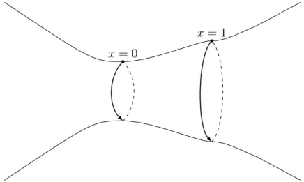
In other words, we gain the full 1/2 of a derivative of local smoothing in thex direction, but we only gain 1/(m+ 1) derivatives of local smoothing in theθ direction. Note that as the trapping becomes more stable, the local smoothing gained in the θ direction goes to 0.
x= 1
x= 0
Figure 4.1: A piece of the manifold with trapped geodesics at x= 0 andx= 1.
rotated can be written explicitly as
A2(x) = 1 + Z x
0
y2m1−1(y−1)2m2/(1 +y2)m1+m2−1dy,
where m1 and m2 are positive integers. To make things more clear, note that
A2 ∼
1 +x2m1, x∼0
C1+c2(x−1)2m2+1, x∼1 x2, |x| → ∞.
The point is that the manifold has two periodic geodesics. The one at x = 0 is the type studied in [CW13]. For this manifold, the local smoothing result states that for solutions of the Schr¨odinger equation, there existsC > 0 such that
Z T
0
k hxi−1∂xuk2+k hxi
−3/2
∂θuk2dt ≤CT
k hDθiβ(m1,m2)u0k2+k hDxi1/2u0k2
where
β(m1, m2) = max
m1 m1+ 1,
2m2+ 1
2m2+ 3
.
The meaning of β(m1, m2) is that the overall degree of local smoothing is determined by
whichever trapped geodesic gives us worse local smoothing.
It should be noted that the results of [CW13] and [CM14] are sharp and show that no better (lower) power of hDθi is possible.
Finally, [Chrar] gives details of the connection between resolvent estimates for the Lapla-cian and local smoothing, and a detailed exposition of how the results obtained in [CW13] and [CM14] can be combined via “gluing” to prove local smoothing results for a wide variety of warped product manifolds.
CHAPTER 5
Conformal perturbations of surfaces of revolution
The previous results mentioned above essentially complete the study of local smoothing for the Schr¨odinger equation on surfaces of revolution (and warped product manifolds in general). All of these results are essentially 1 dimensional, thanks to the decomposition into Fourier modes. The degree of local smoothing for the Schr¨odinger equation on higher dimensional manifolds with trapping is largely unknown with a few exceptions. These exceptions are the case of stable trapping ([Chrar]), the case of non-degenerate hyperbolic trapping (see [Bur04], [Chr07], [Chr08], [Chr11], and [Dat09]), and [Gou12]. We study local smoothing on surfaces which are conformal perturbations of surfaces of revolution.
Recall that a surface of revolution is the manifold M =Rx×Rθ/2πZ endowed with the
metric
g0 =dx2+A2(x)dθ2,
where A >0. We consider conformal perturbations of this metric in which the metric is of the form
gs =esf(x,θ)g0,
where f(x, θ) is a smooth function, compactly supported in x. Note that
∆gs =e −sf∆
g0.
for surfaces of revolution.
If our perturbation function f has appropriate conditions placed on it, one expects that it will have little effect on the dynamics near the trapped set and thus little effect on the local smoothing. In fact, it is reasonable to expect that the perturbation could make the dynamics less stable and thus lead to greater local smoothing, though this is beyond our scope.
Theorem 5.0.1. Let >0 and let M =Rx×Rθ/2πZ endowed with the metric
g =esf(x,θ)(dx2+A2(x)dθ2),
where
A(x) = (1 +x2m)1/2m
and f ∈C∞(M) is compactly supported in x and satisfies
|∂xj∂θkf| ≤C|x|2m−1
for x small and j, k ≤N for sufficiently large N =N(m, ) where j+k ≥1. Suppose also that s >0 is sufficiently small. Let
r= m
m+ 1 +.
Then there exists CT >0 such that
Z T
0
k hxi−1∂xuk2+k hxi
−3/2
∂θuk2dt ≤CT(ku0k2H1/2
x
+ku0k2Hr θ)
for all u solving the Schr¨odinger equation
(Dt−∆g)u= 0
Remark. In the unperturbed case, there is a gain of
1
m+ 1
derivatives, whereas in our case there is the gain of
1
m+ 1 −
derivatives.
This is because we have chosen to avoid the marginal calculus used in [CW13], in order to ensure gains (in terms of θ derivatives) in symbol expansions, so that the many extra terms introduced by the factor e−sf are easier to control.
Remark. Note that we do not require any bound onf itself, only on its derivatives.
Remark. The intuitive reason for our condition on derivatives of f is that in general the degenerate trapping found in the unperturbed manifold is unstable under perturbation, and could potentially be perturbed into much worse trapping, for which the result would not hold.
We also note that non-degenerate hyperbolic trapping is stable under perturbation, so there is no corresponding result in that situation. In fact, the case of non-degenerate hyperbolic trapping has been explored in much greater generality (see [Chr11]). In addition, non-degenerate hyperbolic trapping can be defined independent of coordinates, so our methods which depend heavily on explicitly coordinates would not apply.
The Laplacian ∆g0 on the unperturbed metric is given by
∆g0 =∂x2+A
−2(x)∂2
θ +A
−1(x)A0
(x)∂x.
Define
by
L1u(x, θ) =A1/2(x)u(x, θ)
and define
L2 :L2(esfdxdθ)→L2(dxdθ)
by
L2u(x, θ) = esf /2u.
Let ˜∆ = L2L1∆gL−11L
−1 2 . Let
V1(x) =
1 2A
00(x)A−1(x)−1
4(A
0(x))2A−2(x)
We compute ˜∆ explicitly and find
˜
∆u=e−sf /2 ∂x2+A−2∂θ2−V1(x)e−sf /2
=e−sf ∂x2+A−2∂θ2
+e−sf(−sfx∂x−A−2sfθ∂θ−(s/2)fxx+ ((s/2)fx)2−A−2(s/2)fθθ+A−2((s/2)fθ)2) −e−sfV1(x).
We note that
(e−sf(ξ2+A−2(x)η2+V1(x)))w =−∆˜
Let
Q=−(e−sf(ξ2+A−2η2))w
and
so that
Q=e−sf(∂x2+A−2∂θ2) +R.
Then Q is essentially self-adjoint and R consists of the lower order parts of the operator. Below we will commute with an operator B involving only 1 derivative. Commuting B
and e−sfV
1(x) will produce a bounded function and no derivatives, or in other words an L2
bounded operator. This can then easily absorbed into the upper bound of ku0k2H1/2, as will be done with many other remainder terms below. Thus proving the result for Q will prove the result for ˜∆. Conjugating back then proves the result for ∆g. For this reason, we will leave out V1(x) in the computations below and work withQ.
5.1 Positive Commutator
We begin by making the same positive commutator argument as in [CW13]. By commuting the operator we are interested in, Q, with an appropriate operator B we are able to prove the local smoothing estimate away from x= 0.
We have
Q=e−sf(∂x2+A−2∂θ2) +R.
For our commutant we choose
We begin by commuting the two operators to find
[Q, B] =e−sf(∂x2+A−2∂θ2)[arctan(x)∂x] (5.1) −arctan(x)∂x[e−sf(∂x2 +A
−2∂2
θ)] + [R, B] =e−sf
arctan(x)∂x3+ 2hxi−2∂x2− 2x (1 +x2)2∂x
+e−sfA−2arctan(x)∂θ2∂x + arctan(x)sfxe−sf(∂x2+A
−2 ∂θ2)
+ arctan(x)e−sf(−∂x3−A−2∂θ2∂x+ 2A0A−3∂θ2) + [R, B] =e−sf
2hxi−2∂x2 − 2x
(1 +x2)2∂x+sfxarctan(x)(∂ 2
x+A
−2 ∂θ2) + arctan(x)2A0A−3∂2θ
+ [R, B].
Now that we are done with the preliminary computations, we begin the argument proper by assuming that u satisfies the Schr¨odinger equation
(Dt−Q)u= 0,
u(0, x, θ) =u0.
Using that, we write down the following expression which equals 0:
0 = Z T
0
hB(Dt−Q)u, ui − hBu,(Dt−Q)ui dt.
In order to make our commutator term appear, we next need to integrate by parts in the second term and obtain
0 = Z T
0
hB(Dt−Q)u, ui − h(Dt−Q)Bu, ui dt+ ihBu, ui| T
We combine the terms involving Dt, Q, and B. This results in
0 = Z T
0
hB(Dt−Q)−(Dt−Q)Bu, ui dt+ ihBu, ui| T
0 .
Finally, we note that these combined terms are precisely the commutator we computed above, and we end up with the equation
0 = Z T
0
h[Q, B]u, ui+ihBu, ui|T0 .
Next we write out the commutator and move the terms we are interested in bounding below to the left hand side. The terms we are interested in bounding below are those which appear most similar to the terms in the final local smoothing estimate. In particular, they are the terms which involve 2 derivatives, but do not contain a factor of s coming from the perturbation. This results in the equation
Z T
0
−e−sf2hxi−2∂x2u, u −
e−sfarctan(x)2A0A−3∂θ2u, u
dt
=− Z T
0
e−sf
2x
(1 +x2)2∂x+sfxarctan(x)(∂ 2
x+A
−2
∂θ2) + [R, B]
u, u
dt
− ihBu, ui|T0 .
bound. Starting with the term involving derivatives of x, we first integrate by parts to find
−
e−sf2hxi−2∂x2u, u =∂xu,(∂x[2e−sfhxi
−2 u].
Next we use the product rule to find that this equals
ke−sf /2hxi−1∂xuk2+
∂xu,
−2sfxe−sfhxi
−2− 4xe−sf
(1 +x2)2
u
.
We move the second term to the right hand side and bound it above. First we note that the function
−2sfxe−sfhxi
−2− 4xe−sf
(1 +x2)2
and all of its derivatives are bounded. We can then split the ∂x across both parts of the inner product an obtain an upper bound ofCkuk2
H1/2 as follows: First we apply the operator hDxi
1/2
hDxi
−1/2
, and then we use integration by parts. This term then equals
hDxi−1/2∂xu,
hDxi1/2((−2sfxe−sfhxi
−2
− 4xe
−sf (1 +x2)2
u)
.
Using the Cauchy-Schwarz inequality we are able to bound this from above by
Ck hDxi−1/2∂xukL2k
hDxi1/2((−2sfxe−sf hxi
−2
− 4xe
−sf (1 +x2)2
u)kL2
Both of these terms are bounded by CkukH1/2, giving us the total bound above by Ckuk2 H1/2 as desired.
Next we move on to the term involving derivatives of θ and proceed similarly. We have
e−sfarctan(x)A0A−3∂θ2u, u =
e−sfarctan(x)x2m−1(1 +x2m)−1/m−1∂θu, ∂θu
−sfθe−sfarctan(x)x2m−1(1 +x2m)−1/m−1∂θu, u
The term involving only a single θ derivative is moved to the right hand side and bounded above by kuk2
H1x,θ/2, just as we did for the terms involving only a single x derivative above. Thus far we have proven the inequality
Z T
0
ke−sf /2hxi−1∂xuk2L2 +
e−sfarctan(x)x2m−1(1 +x2m)−1/m−1∂θu, ∂θu
dt (5.2)
≤ | hBu, ui |
0
+| hBu, ui | T + Z T 0
∂xu,
−2sfxe−sfhxi
−2
− 4xe
−sf (1 +x2)2
u +
sfθe−sf arctan(x)A0A−3∂θu, u
−
e−sf
2x
(1 +x2)2∂x+sfxarctan(x)(∂ 2
x+A
−2∂2
θ) + [R, B]
u, u
dt
The first term on the left hand side is already written as a norm. For the second term, we need to do a bit of work before it can be bounded below by a norm. Note that
e−sf|x|2mhxi−2m−3
∂θu, ∂θu
≤C
e−sfarctan(x)x2m−1(1 +x2m)−1/m−1∂θu, ∂θu
,
So we may bound (5.2) below by
c
Z T
0
ke−sfhxi−1∂xukL22 +ke−sf|x|mhxi
−m−3/2
∂θuk2L2dt, (5.3)
for some c >0.
Finally, we can drop the factors of e−sf by using the fact that f is compactly supported and hence e−sf is bounded below by somec >0. Thus the lower bound is
c
Z T
0
k hxi−1∂xukL22 +k|x|mhxi
−m−3/2
So far we have shown
c
Z T
0
ke−sf /2hxi−1∂xukL22 +ke−sf /2|x|mhxi
−m−3/2
∂θuk2L2dt
≤ | hBu, ui | T 0 + Z T 0
∂xu,
−2sfxe−sfhxi
−2− 4xe−sf
(1 +x2)2
u +
sfθe−sfarctan(x)A0A−3∂θu, u
−
e−sf
2x
(1 +x2)2∂x+sfxarctan(x)(∂ 2
x+A
−2∂2
θ) + [R, B]
u, u
dt
In the end, our upper bound will be Cku0k2H1/2. To start, we write out B and apply hDxi−1/2hDxi1/2 as we did above, to find
| hBu, ui |=DhDxi
−1/2
∂xu,hDxi1/2arctan(x)u E
≤ k hDxi
−1/2
∂xukL2k hDxi1/2arctan(x)ukL2.
The operator hDxi
−1/2
∂x is bounded as an operator from H1/2 →L2, so
k hDxi
−1/2
∂xukL2 ≤CkukH1/2.
The operator hDxi
1/2
arctan(x) is a composition of operators in the classes Ψ1/2 and Ψ0, so it is in Ψ1/2, and thus
k hDxi1/2arctan(x)ukL2 ≤CkukH1/2.
We apply this to the inner product hBu, uievaluated at t = 0 andt=T to find
| hBu, ui | T 0
≤C(ku(T,·)k2
H1/2 +ku(0,·)k2H1/2)≤Cku0k2H1/2,
time.
For the next term we use the same trick of applying hDxi
−1/2h
Dxi1/2 to “average” one derivative over both sides of the inner product,
∂xu,
−2sfxe−sfhxi
−2
− 4xe
−sf (1 +x2)2
u = hDxi
−1/2
∂xu,hDxi
1/2
−2sfxe−sfhxi
−2
− 4xe
−sf (1 +x2)2
u .
Using the same argument we see that this is controlled by ku0k2H1/2. Then
Z T 0
∂xu,
−2sfxe−sfhxi
−2
− 4xe
−sf (1 +x2)2
u
dt ≤C
Z T
0
kuk2
H1/2dt≤CTku0k2H1/2.
The same argument works as well for each of our terms that involve only one derivative. Because R consists of terms with at most 1 derivative and B involes only 1 derivative, the commutator [R, B] consists of terms involving only a single derivative. The above argument then shows
Z T
0
| h[R, B]u, ui |dt≤CTku0k2H1/2.
That leaves us with an upper bound of
C(T + 1)ku0k2H1/2 + Z T
0
e−sf(sfxarctan(x)(∂x2+A
−2∂2
θ)
dt
The strategy for dealing with these terms with two derivatives is to make use of the fact that s is small to absorb them into the lower bound. We work first with the term involving
x derivatives. We begin by splitting the two derivatives over the two halves of the inner product using integration by parts to find
Z T
0
se−sffxarctan(x)∂x2u, u dt = Z T 0
s∂x(e−sffxarctan(x)u), ∂xu
Next we apply the derivative using the product rule to find that this equals Z T 0
se−sf −s(fx)2arctan(x) +fxxarctan(x) +fxhxi
−2
+fxarctan(x)∂x
u, ∂xu
dt.
For the terms where ∂x has hit something other than u, we are left with an inner product involving only a total of one derivative, and we can use our technique of “averaging” this derivative to bound this by the H1/2 norm. This gives us an upper bound of
CTku0k2H1/2+ Z T
0
se−sffxarctan(x)∂xu, ∂xu
dt.
By making use of the fact that f is compactly supported, we can then bound this above by
CTku0k2H1/2 +Cs Z T
0
k hxi−1∂xuk2L2
The second of these terms may be moved to the lower bound and absorbed, provided that s
is sufficiently small.
We next use essentially the same argument for the term involving two θ derivatives. One difference is that the lower bound involving∂θ vanishes nearx= 0, so there will be a requirement onfx in order to absorb our term involving sinto the lower bound. We begin by using integration by parts and the technique of averaging derivatives to write
Z T
0
e−sfsfxarctan(x)A−2∂θ2)u, u dt =s Z T 0
∂θ(e−sffxarctan(x)A−2u), ∂θu dt =s Z T 0
e−sfarctan(x)A−2(sfθfx+fxθ+fx∂θ)u, ∂θu
dt
≤CTku0k2H1/2 + Z T
0 s
e−sffxarctan(x)A−2∂θu, ∂θu
Next we suppose that
|fx| ≤C|x|2m−1
in a neighborhood of x= 0. Then using also the fact thatf is compactly supported, we have
|sfxarctan(x)| ≤Cs|x|2mhxi
−2m−3 ,
and thus
Z T
0 s
e−sffxarctan(x)A−2∂θu, ∂θu
dt ≤Cs Z T
0
k|x|mhxi−m−3/2
∂θuk2L2dt.
By choosing s sufficiently small we may absorb this into the lower bound. We thus have the estimate
Z T
0
k hxi−1∂xukL22 +k|x|mhxi
−m−3/2
∂θuk2L2dt≤CTku0k2H1/2 (5.5)
This estimate shows that the local smoothing is perfect away from the x= 0, and that we have perfect local smoothing in the xdirection. Next we will work on the local smoothing in the θ direction and near x= 0.
5.2 Estimating in the Frequency Domain
Our plan is to split the function u up based on whether Dx or hDθi is larger, writing
u=u1+u2, so that u2 satisfies the bound
k hDθiu2kL2 ≤ k∂xu2kL2.
the Schr¨odinger equation, there will be additional error terms. The lower bound of
Z T
0
k hxi−1∂xu2k2L2dt
can be bounded from below by
Z T
0
k hxi−1hDθiu2k2L2dt
This gives us a lower bound in the θ direction away from x= 0. However, it is only foru2, and the upper bound will involve a term other than ku0k2
H1/2, due to the fact that u2 does not solve the Schr¨odinger equation. The other term in the upper bound will essentially be
Z T
0
k hxi−2Dθu1k2L2dt.
Thus, we will have reduced the problem to finding an upper bound for u1, which will be the
subject of the remaining sections.
Let ψ(τ) be a bump function with ψ(τ) = 0 for |τ| > 2 and ψ(τ) = 1 for |τ| < 1. We define the operator ψ(Dx/hDθi) as a Fourier multiplier. Let ˆu(t, ξ, η) denote the Fourier transform of u in x and θ. Because θ ∈ S1, η takes integer values. Let F denote also this
Fourier transform:
(Fu)(ξ, η) = Z
R
Z S1
e−ixξe−iθηu(x, θ)dθdx.
LetF−1 denote the inverse. Note that F−1 involves an integral inξ but a sum inη:
(F−1v)(x, θ) = 1
4π2
Z
R
X η∈Z
eixξeiθηv(ξ, η)dξ
We then define
Again suppose usolves
(Dt−Q)u= 0,
u(0, x, θ) =u0.
We will consider u1 =ψ(Dx/hDθi)u and u2 = (1−ψ(Dx/hDθi))u.
While u2 is not a solution to the Schr¨odinger equation, we will show that it is close enough
to a solution for our purposes. We have
(Dt−Q)u2 = (Dt−Q)[(1−ψ(Dx/hDθi))u]
= (1−ψ(Dx/hDθi))(Dt−Q)u+ [Q, ψ(Dx/hDθi)]u = [Q, ψ(Dx/hDθi)]u.
Because this is a commutator term, we know that it is lower order. When the time comes to use this, we will show precisely what is meant by lower order here.
Letting B = arctan(x)∂x as above we repeat the positive commutator argument from above. We begin by simply expanding the commutator to find
Z T
0
h[Q, B]u2, u2i dt=
Z T
0
hQBu2, u2i − hBQu2, u2i dt
Next we want to have bothQ’s be applied to u2 so that we can use what we know aboutu2
and the Schr¨odinger equation.
We then proceed as in the calculations following (5.1) to find
Z T
0
h[Q, B]u2, u2i dt=
Z T
0
hBu2,(Dt−Q)u2i − hB(Dt−Q)u2, u2i
dt
+ihBu2, u2i
T t=0
.
side will need to be bounded from above, in a manner similar to the preceding section. Next we consider
Z T
0
hBu2,(Dt−Q)u2i dt.
We write this as
Z T
0
hxi−1Bu2,hxi(Dt−Q)u2
dt≤C
Z T
0
(k hxi−1Bu2k2L2 +k hxi(Dt−Q)u2k2L2)dt.
Z T
0
k hxi−1Bu2k2dt ≤C
Z T
0
k hxi−1(1−ψ(Dx/hDθi))∂xuk2+k[ψ(Dx/hDθi), ∂x]uk2dt.
Note that [ψ(Dx/hDθi), ∂x] is anL2 bounded operator. Using the inequality we proved in the previous section, we then know
Z T
0
k hxi−1Bu2k2dt ≤
Z T
0
k hxi−1∂xuk2dt+Ckuk2L2 ≤CTku0k2H1/2.
Recall that from the above,
(Dt−Q)u2 = [Q, ψ(Dx/hDθi)]u
= [e−sf(Dx2+A−2Dθ2) +R, ψ(Dx/hDθi)]u = [e−sf, ψ(Dx/hDθi)](Dx2+A
−2D2
θ) +e
−sf[D2
x+A
−2D2
θ, ψ(Dx/hDθi)] + [R, ψ(Dx/hDθi)].
To bound the first of these terms, we make note of the commutator terms. We gain many things from commuting e−sf with ψ(Dx/hDθi). Because f has compact support in x, we have decay inx as quickly as we like. Because of theψ term, we will be working in the region where Dx ∼ hDθi, and we will gain a power of Dx or hDθi. Thus
k hxi[e−sf, ψ(Dx/hDθi)](D2x+A
−2D2
θ)uk ≤Ck hxi
−1
We may then bound RT
0 k hxi
−1
Dxuk2dt byCTku0k2H1/2 as we did before. Next we note that
[Dx2+A−2D2θ, ψ(Dx/hDθi)] = [A−2(x), ψ(Dx/hDθi)]D2θ
We have
hxi[A−2(x), ψ(Dx/hDθi)]Dθ2 =Lhxi
−2
Dθψ˜(Dx/hDθi),
where L is L2-bounded and ˜ψ ∈C∞
0 equals 1 on suppψ. Then
Z T
0
k hxi[A−2(x), ψ(Dx/hDθi)]D2θuk2dt = Z T
0
kLhxi−2Dθψ˜(Dx/hDθi)uk2dt ≤C
Z T
0
k hxi−2Dθψ˜(Dx/hDθi)uk2dt.
Controlling this will be the subject of the next section. The term
Z T
0
hB(Dt−Q)u2, u2i dt =
Z T
0
h(Dt−Q)u2, B∗u2i dt
is controlled in exactly the same fashion. Thus far we have shown
Z T
0
h[Q, B]u2, u2i dt≤CTku0k2H1/2 + Z T
0
k hxi−2Dθψ˜(Dx/hDθi)uk2dt.
Next we use our expansion of [Q, B] given in (5.1) above:
[Q, B] =e−sf
2hxi−2∂x2 − 2x
(1 +x2)2∂x−sfxarctan(x)(∂ 2
x+A
−2(x)∂2
θ) + arctan(x)2A0A−3∂θ2
As in the previous section we have
Z T
0
| h[R, B]u2, u2i |dt≤CTku0k2H1/2.
Next we write
Z T
0
−2e−sfhxi−2∂x2u2, u2
dt= 2 Z T
0
e−sf /2hxi−1∂xu2, ∂x(e−sf /2hxi
−1 u2)
dt
= 2 Z T
0
ke−sf /2hxi−1∂xu2k2dt
+ Z T
0
e−sf /2hxi−1∂xu2, ∂x(e−sf /2hxi
−1
)u2
dt. Note that Z T 0
e−sf /2hxi−1∂xu2, ∂x(e−sf /2hxi
−1
)u2
dt
≤C
Z T
0
k hDxi
−1/2
(e−sf /2hxi−1∂xu2)kk hDxi1/2[(∂xe−sf /2hxi
−1
]u2kdt
≤C
Z T
0
kuk2
H1/2dt ≤CTku0k2H1/2.
The following term is taken care of similarly:
Z T
0
−
e−sfarctan(x)2A0A−3∂θ2u2, u2 dt
= Z T
0
arctan(x)2A0A−3∂θu2, ∂θ(e−sfu2) dt = Z T 0
e−sfarctan(x)2A0A−3∂θu2,(−sfθ+∂θ)u2)
dt.
CTku0k2H1/2. The other term is
Z T
0
e−sfarctan(x)2A0A−3∂θu2, ∂θu2
dt≥c
Z T
0
k|x|mhxi−m−3/2
∂θuk2dt.
The next term we bound from above is
Z T
0
2xhxi−4∂xu2, u2
dt≤CTku0k2H1/2,
again by using our technique of “averaging” half a derivative across the inner product. The remaining terms can be controlled by using our bound from the previous section. First we have
Z T
0
se−sffxarctan(x)∂x2u2, u2
dt = Z T 0 s
∂xu2, ∂x(e−sffxarctan(x)u2)
dt = Z T 0 s
∂xu2, e−sffxarctan(x)∂xu2
dt + Z T 0 s
∂xu2,(∂x(e−sffxarctan(x)))u2
dt
The second term here can be bounded by CTku0k2H1/2 again by averaging the derivative. For the first term, we instead note that
Z T
0 s
∂xu2, e−sffxarctan(x)∂xu2
dt ≤C Z T
0
k hxi−1∂xuk2dt ≤CTku0k2H1/2,
The only remaining term is
Z T
0 s
e−sffxarctan(x)A−2∂θ2u2, u2
dt
= Z T
0 s
e−sffxarctan(x)A−2∂θu2, ∂θu2
dt
+ Z T
0 s
sfθe−sffxarctan(x)A−2∂θu2, u2
dt
The second term is again bounded by CTku0k2
H1/2 by averaging the derivative over the inner product. For the first term we have
Z T
0 s
e−sffxarctan(x)A−2∂θu2, ∂θu2
dt
≤Cs
Z T
0
k|x|mhxi−m−3/2
∂θuk2dt ≤CTku0k2H1/2,
where we have used our condition that |fx| ≤x2m−1 forx near 0, as well as the bound proven in the previous section.
Putting all of this together we end up with
Z T
0
k hxi−1∂xu2k2L2 +k|x|mhxi m−3/2
∂θu2k2L2dt ≤CTku0k2H1/2 +C
Z T
0
k hxi−2Dθψ˜(Dx/hDθi)uk2L2dt.
Finally we make use of the support property of ψ(Dx/hDθi)u. This function cuts
u2 = 1−ψ(Dx/hDθi)u off to where hDθi ≤∂x, so we have
k hxi−1hDθiu2k ≤Ck hxi
−1
Using this lower bound we see that
Z T
0
k hxi−1hDθiu2k2L2dt ≤CTku0k2H1/2+ Z T
0
k hxi−2Dθψ˜(Dx/hDθi)uk2L2dt.
Furthermore let χ(x)≡1 near 0 and have compact support. Then
Z T
0
k hxi−2Dθψ˜(Dx/hDθi)uk2L2dt ≤C
Z T
0
k hxi−2Dθψ˜(Dx/hDθi)χ(x)uk2L2+k hxi
−2
Dθψ˜(Dx/hDθi)(1−χ(x))uk2L2dt
The second of these terms can then be bounded using the bound from the previous section:
Z T
0
k hxi−2Dθψ˜(Dx/hDθi)(1−χ(x))uk2dt≤C Z T
0
hxi−2(1−χ(x))Dθuk2dt ≤
Z T
0
k|x| hxim−3/2∂θuk2dt ≤CTku0k2H1/2.
Thus to finish this part of our estimate need only bound
Z T
0
k hxi−2Dθψ˜(Dx/hDθi)χ(x)uk2L2dt.
Note that by bounding this, we will also bound
Z T
0
k hxi−2Dθχ(x)u1k2L2dt,
5.3 High Frequency Estimate
We have proven our local smoothing estimate outside of a region that is “small” in both space and frequency. This suggests that it will be profitable to work microlocally. To that end, we wish to show that bounding
Z T
0
k hxi−2Dθψ˜(Dx/hDθi)χ(x)uk2L2dt
is equivalent to proving a bound of the form
k(Q+τ)ψχuk ≥ k hDθir˜ψχuk,
for u microlocalized near (x, ξ/hηi) = 0. We do this by using a “T T∗” argument.
The operator to which we apply the argument will be F(t). Define the operator F(t) by
F(t)g =χ(x)ψ(Dx/hDθi)eitQg(x, θ).
We need to determine for which values of r, with 0 ≤ r ≤ 1, we have a bounded map
F :L2xL2θ →L2([0, T])L2xHθr. We have
F∗g = Z T
0
e−i˜tQψ(Dx/hDθi)χ(x)˜g d˜t
and we need to show
F∗ :L2([0, T])L2xHθ−r →L2xL2θ.
Then
F F∗g˜=χ(x)ψ(Dx/hDθi) Z T
0
and we need to show
F F∗ :L2([0, T])L2xHθ−r →L2([0, T])L2xHθr.
We split this expression into two. Let
v1 =
Z t
0
ei(t−˜t)Qψ(Dx/hDθi)χ(x)˜g dt˜
and
v2 = Z T
t
ei(t−˜t)Qψ(Dx/hDθi)χ(x)˜g d˜t.
Then
F F∗g˜=χ(x)ψ(Dx/hDθi)(v1+v2).
We need to show
kχ(x)ψ(Dx/hDθi)vjkL2
tL2xHθr ≤Ck˜gkL2tL2xH
−r θ
forj = 1,2, where we require some assumptions on ˜g which will be included in the statement of our theorem below.
Note that
(Dt+Q)v1 =−iψ(Dx/hDθi)χ(x)˜g
and
(Dt+Q)v2 =iψ(Dx/hDθi)χ(x)˜g.
Let ˆ· denote the Fourier transform in time. Then
If we can prove the bound
kχψvˆjkL2
τL2xHθr ≤Ck˜gkL2τL2xH
−r θ ,
we will have shown that F F∗ : L2tL2xHθ−r → L2tL2xHθr (and thus F : L2xL2θ →L2tL2xHθr) is a bounded operator. To that end, we need to bound the operator
χ(x)ψ(Dx/hDθi)(Q+τ)−1ψ(Dx/hDθi)χ(x)
in the L2xHθr→L2xHθ−r operator norm, uniformly in τ.
This is equivalent to showing that there exists C such that
k hDθi
2r
ukL2
x,θ ≤Ck(Q+τ)ukL2x,θ.
Suppose that |τ| ≥C|η|2. Then by ellipticity we have
k(Q+τ)uk ≥ck hDθi
2 uk.
Hence we need only work where |τ| ≤C|η|2.
Proving this estimate will be the subject of the next section. Proving it will bound
χ(x)ψ(Dx/hDθi)eitQg inL2tL2xHθr, but we are ultimately interested in bounding it inL2tL2xHθ1. To do so, we apply the bound to hDθi1
−r
g, so we will ultimately end up with the bound
Z T
0
k hDθiχ(x)ψ(Dx/hDθi)uk2L2
x,θdt≤Cku0k
2
H1−r.
5.4 Microlocal proof of the Resolvent Estimate
Theorem 5.4.1. Let >0 and letp= ξ2+η2A−2. Suppose f(x, θ)is a compactly supported,
smooth function such that
|∂xj∂θkf| ≤C|x|2m−1
for x small and j, k ≤N for sufficiently largeN = N(m, )and j+k ≥1. Suppose also that
s is sufficiently small. Then there exists c >0 such that
k((e−sfp)w +τ)ukL2
x,θ ≥ck hDθi
2/(m+1)−
ukL2
x,θ,
for all τ, provided that u satisfies the following microlocal support properties: We require that
u be of the form
u=bwu,˜
where b has symbol supported in the region where |(x, ξ/η)| ≤δ/2 for some sufficiently small
δ and |η| ≥M for some sufficiently large M.
Broadly speaking, our proof uses a commutator argument. The basic structure is to make use of the fact that to highest order, the symbol of the commutator of two pseudodifferential operators is given by applying the Hamiltonian vector field of the one symbol to the other symbol. Recall that Q = (e−sfp)w denotes the operator we are interested in. We define a symbol a ∈ S0
such that He−sfpa has the required lower bound. Ignoring the issues of
error terms coming from the pseudodifferential calculus for the moment, we will consider the quantity
h[Q+τ, aw]u, ui,
where a is yet to be determined.
Roughly, this is bounded from above by applying absolute values, expanding the commu-tator, and integrating by parts to give us an upper bound (for now) of
As we stated above, the lower bound makes use of the fact that to highest order, [Q, aw] = (He−sfpa)w. We seek a such that the resulting symbol He−sfpa is of the form η−(ξ2+η2x2m)
at least where x and ξη−1 are small andη is large. We may then use a lower bound on this
operator to achieve a lower bound of
k hDθi1/(m+1)−/2uk2 ≤ |hawu,(Q+τ)ui|.
The bulk of the proof is concerned with dealing with the error terms that turn up in applying the pseudodifferential calculus and terms that appear due to the presence ofe−sf. It is in the process of absorbing these terms that the need for conditions onf become clear. The operator we require a lower bound on is (e−sfp)w+τ. To define the symbol of our commutant a, we first define
Λ(t) = Z t
0
˜
t−1−0
d˜t,
where 0 >0 is sufficiently small. The important facts about Λ(t) is that it is a symbol of
order 0, and Λ(t)∼t near 0.
We will also make use of cutoff functions χ(t) and ˜χ(t). Let χ(t) be a smooth, compactly supported function such that χ(t)≡1 for |t| ≤δ/2 and χ(t) ≡0 for |t| ≥ δ. Let ˜χ(t) be a smooth function such that ˜χ(t)≡0 for |t| ≤M and ˜χ(t)≡1 for|t| ≥2M.
Let
a=χ(x)χ(ξη−1)Λ(x)Λ(ξη−) ˜χ(η)
and note that
|∂xα∂ξβ∂θγ∂ηδa| ≤Cα,β,γ,δhξi
−βh
ηi−δ,
where we have used the fact thatχ(ξη−1) cuts off to where|ξ| ≤ |η|. Because of this inequality, a∈S0
Theorem 5.4.2. Let p, a as above. Then for any >0 there exists c >0 such that
e−sf(He−sfpa)wu, u
≥c(Dθ)−(Dx2+D
2
θx
2m)u, u
− O(k hDθi
−/2
)uk2).
for all u microsupported where |x| ≤δ, |ξη−1| ≤δ, and |η| ≥M for some large M.
Proof. We begin by computing He−sfpa. First recall that
p(x, ξ, θ, η) =ξ2+A−2(x)η2
and
a(x, ξ, θ, η) =χ(x)χ(ξη−1)Λ(x)Λ(ξη−) ˜χ(η).
Note that a does not depend on θ, so no (e−sfp)
ηaθ term will appear. We next compute the necessary derivatives. Recall that the notation for the η derivative actually refers to a difference operator in η.
(e−sfp)x=−2e−sfA−3A0η2−sfxe−sfp, (e−sfp)ξ= 2e−sfξ,
(e−sfp)θ =−sfθe−sfp
ax= [χ0(x)χ(ξη−1)Λ(x)Λ(ξη−) +χ(x)χ(ξη−1)Λ0(x)Λ(ξη−)] ˜χ(η),
aξ= [η−1χ(x)χ0(ξη−1)Λ(x)Λ(ξη−) +η−χ(x)χ(ξη−1)Λ(x)Λ0(ξη−)] ˜χ(η)
aη = Λ(x)(Λ(ξ(η+ 1)−)−Λ(ξη−))χ(x)χ(ξη−1) ˜χ(η)
+ Λ(x)Λ(ξ(η+ 1)−)χ(x)χ(ξ(η+ 1)−1) ˜χ(η+ 1)−χ(ξη−1) ˜χ(η)
Using this computation we write down He−sfpa and split it into two parts. We are only
interested in the behavior of He−sfpa where x is small, ξη−1 is small, and η is large, so we
already proven our local smoothing estimate in these regions, there is no need to apply our resolvent estimate there.
We have
He−sfpa =
2e−sfξ
χ0(x)χ(ξη−1)Λ(x)Λ(ξη−) +χ(x)χ(ξη−1)Λ0(x)Λ(ξη−)
−(−2e−sfA−3A0η2 −sfxe−sfp)
χ(x)χ0(ξη−1)η−1Λ(x)Λ(ξη−) +η−χ(x)χ(ξη−1)Λ(x)Λ0(ξη−)
+ (−sfθe−sfp)Λ(x)
Λ(ξ(η+ 1)−)−Λ(ξη−)
χ(x)χ(ξη−1)
( ˜χ(η))
+ (−sfθe−sfp)Λ(x)Λ(ξ(η+ 1)−)χ(x)
χ(ξ(η+ 1)−1) ˜χ(η+ 1)−χ(ξη−1) ˜χ(η).
We collect the terms involving derivatives of χor ˜χ and write
He−sfpa=
2ξΛ0(x)Λ(ξη−)−2A−3A0η2−Λ(x)Λ0(ξη−) −sfxpη−Λ(x)Λ0(ξη−)−sfθpΛ(x)
Λ(ξ(η+ 1)−)−Λ(ξη−)
×e−sfχ(x)χ(ξη−1)( ˜χ(η)) +r,
where
suppr⊂ {|x| ≥δ/2} ∪ {|ξ| ≥δ|η|/2} ∪ {|η| ≤2M}.
We use g to denote the part of He−sfpa to which we devote most of our efforts. Let
We use ˜g to denote the terms in which derivatives have hit e−sf:
˜
g =
−sfxpη−Λ(x)Λ0(ξη−) (5.6)
−sfθpΛ(x)
Λ(ξ(η+ 1)−)−Λ(ξη−)
e−sfχ(x)χ(ξη−1) ˜χ(η),
so
He−sfpa=g+ ˜g+r.
Our goal is, roughly, to show that ˜g can be absorbed intog and that g is bounded below by a small multiple of η−(ξ2+η2x2m).
We begin by bounding ˜g from above. Because we will only apply this result to functions which are microlocally supported in the region where χ(x) = 1, χ(ξη−1) = 1, and ˜χ(η) = 1,
we omit the χ and ˜χ factors. We start with the first term in (5.6):
|sfxpη−Λ(x)Λ0(ξη−)e−sf| ≤C|sfxη−(ξ2+η2A−2(x))Λ(x)Λ0(ξη−)| ≤C|sfxη2−Λ(x)Λ0(ξη−)|,
where we have used the fact that |ξ| ≤Cη.
For the next term in (5.6) we first use the mean value theorem to note that
Λ(ξ(η+ 1)−)−Λ(ξη−)=
Z ξ(η+1)−
ξη−
hti−1−0 dt
≤C|ξ|(η+ 1)−−η−
ξη−−1−0
≤C|ξ||η−1−|
Thus
−sfθpΛ(x)
Λ(ξ(η+ 1)−)−Λ(ξη−)
e−sf
≤Csfθη−1−(ξ2+η2A−2(x))ξΛ(x)
ξη−−1−0
≤C|sfθη2−Λ(x)
ξη−−1−0 |,
so
|˜g| ≤ |s|(|fx|+|fθ|)|η2−Λ(x)|
ξη−−1−0. (5.7)
We need to write g in a more useful form. To get started, we recall that the definition of Λ is
Λ(t) = Z t
0
˜
t−1−0 d˜t,
so Λ0(t) = hti−1−0, and
g = (2ξhxi−1−0Λ(ξη−) + 2η2−A−3(x)A0(x)Λ(x)ξη−−1−0)e−sfχ(x)χ(ξη−1) ˜χ(η).
We will assume throughout that |x| ≤δ/2, |ξη−1| ≤δ/2, and |η| ≥ M because we will be applying our operators to functions microlocally cutoff near here. In this region, χ(x) = 1,
χ(ξη−1) = 1, and ˜χ(η) = 1.
We first break g up into two parts:
g = (2ξhxi−1−0Λ(ξη−) + 2η2−A−3(x)A0(x)Λ(x)ξη−−1−0)e−sf
where
g1 = 2ξhxi
−1−0
Λ(ξη−)e−sf, g2 = 2η2−A−3(x)A0(x)Λ(x)
ξη−−1−0
e−sf.
Before bounding g from below, we note how ˜g may be absorbed intog. From (5.7) we see that
˜
g ≤C|s|g2
as long as |fx| ≤CA0(x) and |fθ| ≤CA0(x). This is satisfied as long as|fx| ≤C|x|2m−1 and
|fθ| ≤C|x|2m−1.
We will consider two cases. In the first case we make the assumption that ξη− ≤δ. We are working where Λ is only applied to small quantities, and for |t| small Λ(t) =t+O(t3)
and hti−1−= 1 +O(t2).
We write out g1. Because ηis relatively large and ξ is relatively small, the most important
term will end up being 2η−ξ2e−sf. Below we will show how the other terms may be absorbed. We separate out this term by writing
g1 = (2ξ(1 +O(x2))(ξη−+O((ξη−)3)e−sf
= 2ξ2η−(1 +O(x2))(1 +O((ξη−)2))e−sf
= 2η−ξ2e−sf +O(x2ξ2η−) +O(ξ4η−3) +O(ξ4η−3x2) = 2η−ξ2e−sf +ξ2η− O(x2) +O((ξη−)2)
where we have used the fact that there exists C such that e−sf(x,θ) ≤C. Because |x| ≤δ and |ξη−| ≤δ, we then have
Similarly, for g2, the most important term in the expansion will be 2η−(ηxm)2e−sf. Recall
that A(x) = (1 +x2m)1/2m. Here we use Taylor’s theorem to expand A−3(x)A0(x) and write
g2 = 2η2−A−3(x)A0(x)(x+O(x3))(1 +O((ξη−)2)))e−sf
= 2η2−(x2m−1 +O(x4m−1))x(1 +O(x2))(1 + (O((ξη−)2)))e−sf
= 2η−(ηxm)2e−sf + 2η2−x2m (O(x4m) +O((xmξη−)2).
Again using that |x| ≤δ and |ξη−| ≤δ, we have
g2 = 2η−(ηxm)2e−sf(1 +O(δ2)).
Because |˜g| ≤C|s|g2, we then have g2 + ˜g =g2(1 +O(s)), hence
g2+ ˜g = 2η−(ηxm)2e−sf(1 +O(δ2) +O(s))
We can thus write
g+ ˜g = 2e−sfη−(ξ2+η2x2m)(1 +O(δ2) +O(s))
as long as |ξη−| ≤δ.
We move on to our other case, where |ξη−| ≥ δ. Our cutoff functions still allow us to assume that |x| ≤δ, |ξη−1| ≤δ, and |η| is large.
In this region, we will show that g+ ˜g is elliptic. We will consider two cases, based on the size of x relative to the size ofξη−.
We first note that g1, g2 ≥0. Also note using the bound on ˜g given by (5.7) that
g1 +g2+ ˜g =g1+g2(1 +O(s))≥g1+ (1−C|s|)g2 ≥c(g1+g2).
Suppose |x|1+0 ≥ |ξη−| ≥δ.
g2 = 2e−sfη2−A−3(x)A0(x)Λ(x)
ξη−−1−0
= 2e−sfη2−x2m(1 +O(x2m))(1 +O(x2))
ξη−−1−0 ≥ce−sfη2−x2m(1 +O(x2))ξη−−1−0
≥cη2−x2m|ξη−|−1−0 ≥cη2−x2m|x|−(1+0)2 ≥cη2−.
On the other hand, if |ξη−| ≥ |x|1+0, but still |ξη−| ≥δ, then
g1 = 2e−sfξhxi
−1−0
Λ(ξη−) ≥cξΛ(ξη−)
≥cη.
Hence g ≥cη.
In either case, we find that in this region g ≥cη and hence ˜g+g ≥cη. Considering both cases, there thus exists a σ >0 such that if
h(g+ ˜g)wu, ui ≥σk hDθi/2uk2
then u is microlocally supported only in the region where |ξη−| ≤δ. We have shown that there exists c > 0 such that here we may write
This then allows us to write
g+ ˜g =η−(ξ2+η2x2m)K2,
where K is a strictly positive symbol. Because we are using the Weyl quantization here, this quantizes as
Opw(K)∗(Dθ)−(D2x+D
2
θx
2m) Opw(K) +O(hD θi
− ).
Thus, for umicrosupported in this region,
h(g+ ˜g)wu, ui ≥
(Dθ)−(Dx2 +D2θx2m)u, u
− kO(hDθi
−/2
)uk2
We thus have
(He−sfpa)wu, u
≥
(Dθ)−(Dx2 +Dθ2x2m)u, u
− O(k hDθi
−/2 uk2).
Proof of Theorem 5.4.1. In the symbol calculus, the commutator [(e−sfp)w, aw] has principal symbol He−sfpa, but we will still need to control the remaining terms. Let
R1 = [(e−sfp)w, aw]−(He−sfpa)w.
Then we have
[(e−sfp)w+τ, aw] = (He−sfpa)w+R1.
Applying this to u and taking an inner product withu we find the equality
[(e−sfp)w+τ, aw]u, u=(He−sfpa)wu, u
We can then apply the above Theorem 5.4.2 to find
[(e−sfp)w+τ, aw]u, u≥c
hDθi
−
(D2x+D2θx2m)u, u−Ck hDθi
−/2
uk2 (5.8)
− |hR1u, ui|
Our goal is to bound hR1u, ui from above in such a way that it can be absorbed into the
term chDθi
−
(D2x+D2θx2m)u, u.
The commutator [(e−sfp)w, aw] has symbol given by N
X k=0
ik k!σ(D)
kh
p(x, ξ, θ, η)a(˜x,ξ,˜θ,˜ η˜)−(e−sfp)(˜x,ξ,˜θ,˜ η˜)a(x, ξ, θ, η) i diag
+O(hηi−N),
where diag
denotes evaluation along the diagonal, i.e. x= ˜x,ξ = ˜ξ, θ = ˜θ, and η= ˜η. The bound on the error term is a result of the symbol class we are working in. Recall also from Theorem 2.2.3 that
A(D) = 1
2 h(Dξ, Dη),(Dx˜, Dθ˜)i −
(Dx, Dθ),(D˜ξ, Dη˜
.
The first non-zero term in this expansion is He−sfpa. Because we are using the Weyl
calculus, there are no even terms. Therefore, when applying this symbol expansion to write down R1, the first term is
i3
3!A(D)
3h(e−sfp)(x, ξ, θ, η)a(˜x,ξ,˜η˜)−(e−sfp)(˜x,ξ,˜θ,˜ η˜)a(x, ξ, η)i diag .
Before expanding A(D)3, we note that a does not depend on θ, so there will be no terms
a factor of s. When this is the case, we can bound above by
C|sf∗η2−Λ(x)|, (5.9)
where f∗ denotes some (first, second, or third) derivative of f. As long as we require
|f∗| ≤Cx2m−1 we find that (5.9) is bounded above by C|s||η2−|x2m, and will be no problem
to absorb.
The remaining term occurs when three x derivatives all hit p. This term is
Ce−sf(Dx3p)(Dξ3a) = Ce−sf(A−2)000(x)η2−3Λ(x)Λ000(ξη−)χ(x)χ(ξη−1)(1−χ(η)) +r2,
where
suppr2 ⊂ {|x| ≥δ} ∪ {|ξ| ≥δ|η|} ∪ {|η| ≥δ}.
Because we will be applying our estimate only on functions microlocally supported away from the support of r2, it will pose no problem to absorb this term. For now, we simply carry
this term along. We first note that
|(A−2)000| ≤C|x|2m−3.
Next note that
|Λ(x)| ≤ |x|.
Hence
C(A−2)000(x)η2−3Λ(x)Λ000(ξη−)χ(x)χ(ξη−1)(1−χ(η))≤Cx2m−2η2−3.
Next we need to control the symbol Cx2m−2η2−3. When |x|−1 ≤c
0|η|, we have