Vol 8, No 7 (2017)

Available online throug

ISSN 2229 – 5046

COMPARATIVE STUDY OF HIGHER DEGREE SPLINE SOLUTIONS

OF LINEAR SEVENTH ORDER BOUNDARY VALUE PROBLEMS

PARCHA KALYANI*

_,

_{MIHRETU NIGATU LEMMA}

_{AND DEJENE BEKELE FEYISA}

1

_{Geetanjali College of Engineering and Technology, India.}

2,3

_{School of Mathematical & Statistical Sciences, Hawassa University, Hawassa, Ethiopia.}

(Received On: 01-07-17; Revised & Accepted On: 24-07-17)

ABSTRACT

I

numerical solutions of linear boundary value problems of order seven. Two numerical examples have been considered to illustrate the efficiency and implementation of the method. Numerical solutions are computed at different step lengths and compared with exact solutions. Absolute errors are also calculated. The results are tabulated and pictorially illustrated. Further the results are compared with the methods developed in [10 and 11].

Key words: Spines; Boundary value problems; Numerical results.

1. INTRODUCTION

Boundary value problems (BVPs) for ordinary differential equations (ODEs) are used as mathematical models in a wide variety of disciplines including biology, physics, and engineering [3]. Over the years, there are several authors who study on these types of boundary value problems. There are several methods, such as Finite difference method, Finite element method, Orthogonal splines, Collocation, and etc, to discrete the boundary value problems.Boundary value problems (BVPs) can be used to model several physical phenomena. For example, when an infinite horizontal layer of fluid is heated from below and is subject to the action of rotation, instability sets in. When this instability sets in as ordinary convection, the ordinary differential equation is sixth order and when this instability sets in as over stability, it is modeled by an eighth-order ordinary differential equation [15].

The theory of seventh order boundary value problems is not much available in the numerical analysis literature. The seventh order boundary value problems generally arise in modeling induction motors with two rotor circuits [12]. Siddiqi and Akram [13] presented the solutions of fifth and sixth order boundary value problems using non-polynomial

spline. Mohyud-Din et al. [9] used variation of parameters method for solving fifth order boundary value problems. In

[1] Akram and Rehman solved the fifth order boundary value problems using Reproducing Kernel space method. Akram and Siddiqi [2] presented the solution of seventh order boundary value problem using octic spline. Rashidina

et al. [8] used spline collocation method for the solution of higher order linear boundary value problems. Sastry [14],

Schoenberg [5, 6] made great contributions in the development of splines. Convergence properties of the cubic spline method have been discussed by Ahlberg and Nilson [7]. Numerical solution of value and initial boundary-value problems using spline functions has been given in [4].

In this work we construct tenth degree splines by using Bickley’s method [16] and apply it to the linear seventh order Boundary value problem. The work has been illustrating through examples with different step lengths.

2. CONSTRUCTION OF TENTH DEGREE SPLINE FUNCTION

Assume the interval [𝑥_0,𝑥_𝑛] is divided in to 𝑛 sub intervals with grid points 𝑥₀ ,𝑥₁ ,𝑥₂, 𝑥₃, … 𝑥_𝑛

The function 𝑢(𝑥) in the interval [𝑥_0,𝑥₁], is represent by tenth degree spline in the form

𝑠(𝑥) =𝑎+𝑏(𝑥 − 𝑥0) +𝑐(𝑥 − 𝑥0)2+𝑑(𝑥 − 𝑥0)3+𝑔(𝑥 − 𝑥0)4+𝑗(𝑥 − 𝑥0)5+𝑘(𝑥 − 𝑥0)6

+𝑙(𝑥 − 𝑥₀)7+𝑡(𝑥 − 𝑥₀)8+𝑣(𝑥 − 𝑥₀)9+ 𝑤₀(𝑥 − 𝑥₀)10. (1)

Corresponding Author: Parcha Kalyani*

_,

For the next interval [𝑥_1,𝑥₂] we add a term w₁(𝑥 − 𝑥₁)10,

Going on in to the next interval [𝑥_2,𝑥₃] add another term w₂(𝑥 − 𝑥₂)10and so on until we reach 𝑥_𝑛 hence the function

𝑠(𝑥) represents in the form

𝑠(𝑥) =𝑎+𝑏(𝑥 − 𝑥0) +𝑐(𝑥 − 𝑥0)2+𝑑(𝑥 − 𝑥0)3+𝑔(𝑥 − 𝑥0)4+𝑗(𝑥 − 𝑥0)5+𝑘(𝑥 − 𝑥0)6

+𝑙(𝑥 − 𝑥₀)7+𝑡(𝑥 − 𝑥₀)8+𝑣(𝑥 − 𝑥₀)9+∑𝑛−1_𝑖=0𝑤_𝑖 (𝑥 − 𝑥_𝑖)10. (2)

𝑠(7)_{(𝑥) = 5040𝑙+ 40320𝑡(𝑥 − 𝑥}

0) + 181440𝑣(𝑥 − 𝑥0)2+ 604800∑𝑖=0𝑛−1𝑤𝑖 (𝑥 − 𝑥𝑖)3 (3)

2.1 Method of obtaining the solution of seventh order boundary value problem using tenth degree spline function

Consider the linear seventh order differential equation

𝑦(7)_{(𝑥) +𝑓(𝑥)𝑦(𝑥) =𝑟(𝑥), (4)}

with boundary conditions

𝑦(𝑥0) =𝛽, 𝑦(𝑥𝑛) =𝛾, 𝑦′ (𝑥0) =𝛽′, 𝑦′(𝑥𝑛) = 𝛾′, 𝑦′′(𝑥0) = 𝛽′′, 𝑦′′(𝑥𝑛) = 𝛾′′, 𝑦′′′(𝑥0) = 𝛽′′′, (5)

From (5), and taking spline approximation in (4) at 𝑥=𝑥_𝑖 𝑓𝑜𝑟 𝑖= 0,1, 2, 3, 4, 5, 6, … ,𝑛 we get (𝑛+ 8) equations in

(𝑛+ 10) unknowns𝑎,𝑏,𝑐,𝑑,𝑔,𝑗,𝑘,𝑙,𝑡,𝑣,𝑤₀, 𝑤₁, 𝑤₂, 𝑤₃, 𝑤₄ … ,𝑤_𝑛−1.

After determining these unknowns we substitute them in (2) and thus get the tenth degree spline approximation of

𝑦(𝑥). Substituting (2) and (3) in the differential equation (4) at 𝑥=𝑥_𝑚 where 𝑚= 0,1,2,3, …𝑛 then we get the following

𝑎𝑓(𝑥𝑚) +𝑏𝑓(𝑥𝑚)(𝑥𝑚− 𝑥0) +𝑐𝑓(𝑥𝑚)(𝑥𝑚− 𝑥0)2+𝑑𝑓(𝑥𝑚)(𝑥𝑚− 𝑥0)3+𝑔𝑓(𝑥𝑚)(𝑥𝑚− 𝑥0)4 +𝑗𝑓(𝑥𝑚)(𝑥𝑚− 𝑥0)5+𝑘𝑓(𝑥𝑚)(𝑥𝑚− 𝑥0)6 +𝑙[𝑓(𝑥𝑚)(𝑥𝑚− 𝑥0)7+ 5040]

+𝑡[𝑓(𝑥𝑚)(𝑥𝑚− 𝑥0)8+ 40320(𝑥𝑚− 𝑥0)] +𝑣[𝑓(𝑥𝑚)(𝑥𝑚− 𝑥0)9+ 181440(𝑥𝑚− 𝑥0)2]

+∑𝑛−1𝑖=0𝑤𝑖 [𝑓(𝑥𝑚)(𝑥𝑚− 𝑥𝑖)10+ 604800(𝑥𝑚− 𝑥𝑖)3] =𝑠(𝑥𝑚). (6)

From the boundary conditions (5) we obtain

𝑦(𝑥0) =𝛽,

𝛽 =𝑎+𝑏(𝑥 − 𝑥0) +𝑐(𝑥 − 𝑥0)2+𝑑(𝑥 − 𝑥0)3+𝑔(𝑥 − 𝑥0)4+𝑗(𝑥 − 𝑥0)5+𝑘(𝑥 − 𝑥0)6 +𝑙(𝑥 − 𝑥0)7+𝑡(𝑥 − 𝑥0)8+𝑣(𝑥 − 𝑥0)9+∑𝑛−1𝑖=0𝑤𝑖 (𝑥 − 𝑥𝑖)10,

𝑎=𝛽. (7)

𝑦(𝑥𝑛) =𝛾,

𝑎+𝑏(𝑥𝑛 − 𝑥0) +𝑐(𝑥𝑛 − 𝑥0)2+𝑑(𝑥𝑛 − 𝑥0)3+𝑔(𝑥𝑛 − 𝑥0)4+𝑗(𝑥𝑛 − 𝑥0)5+𝑘(𝑥𝑛 − 𝑥0)6 +𝑙(𝑥𝑛 − 𝑥07+𝑡𝑥𝑛−𝑥08+𝑣𝑥𝑛−𝑥09+𝑖=0𝑛−1𝑤𝑖𝑥𝑛−𝑥𝑖 10 =𝛾. (8)

𝑦′_(𝑥

0) = 𝛽′,

𝛽′ _{=𝑏+ 2𝑐(𝑥 − 𝑥}

0) + 3𝑑(𝑥 − 𝑥0)2+ 4𝑔(𝑥 − 𝑥0)3+ 5𝑗(𝑥 − 𝑥0)4+ 6𝑘(𝑥 − 𝑥0)5 +7𝑙(𝑥 − 𝑥0)6 + 8𝑡(𝑥 − 𝑥0)7+ 9𝑣(𝑥 − 𝑥0)8+ 10∑𝑛−1𝑖=0𝑤𝑖 (𝑥 − 𝑥𝑖)9,

𝑏=𝛽′_{. (9)}

𝑦′_(𝑥

𝑛) = 𝛾′,

𝑏+ 2𝑐(𝑥𝑛 − 𝑥0) + 3𝑑(𝑥𝑛 − 𝑥0)2+ 4𝑔(𝑥𝑛 − 𝑥0)3+ 5𝑗(𝑥𝑛 − 𝑥0)4+ 6𝑘(𝑥𝑛 − 𝑥0)5

+7𝑙(𝑥𝑛 − 𝑥0)6 + 8𝑡(𝑥𝑛 − 𝑥0)7+ 9𝑣(𝑥𝑛 − 𝑥0)8+ 10∑𝑛−1𝑖=0𝑤𝑖 (𝑥𝑛 − 𝑥𝑖)9=𝛾′. (10)

𝑦′′_(𝑥

0) = 𝛽′′,

𝛽′′_{= 2𝑐 + 6𝑑(𝑥 − 𝑥}

0) + 12𝑔(𝑥 − 𝑥0)2+ 20𝑗(𝑥 − 𝑥0)3+ 30𝑘(𝑥 − 𝑥0)4+ 42𝑙(𝑥 − 𝑥0)5 +56𝑡(𝑥 − 𝑥0)6+ 72𝑣(𝑥 − 𝑥0)7+ 90∑𝑛−1𝑖=0𝑤𝑖(𝑥 − 𝑥𝑖)8,

𝑦′′_(𝑥

𝑛) = 𝛾′′,

𝛾′′ _{= 2𝑐 + 6𝑑(𝑥 − 𝑥}

0) + 12𝑔(𝑥 − 𝑥0)2+ 20𝑗(𝑥 − 𝑥0)3+ 30𝑘(𝑥 − 𝑥0)4+ 42𝑙(𝑥 − 𝑥0)5 +56𝑡(𝑥 − 𝑥0)6+ 72𝑣(𝑥 − 𝑥0)7+ 90∑𝑛−1𝑖=0𝑤𝑖(𝑥 − 𝑥𝑖)8,

2𝑐 + 6𝑑(𝑥𝑛 − 𝑥0) + 12𝑔(𝑥𝑛 − 𝑥0)2+ 20𝑗(𝑥𝑛 − 𝑥0)3+ 30𝑘(𝑥𝑛 − 𝑥0)4+ 42𝑙(𝑥𝑛 − 𝑥0)5

+56𝑡(𝑥𝑛 − 𝑥0)6+ 72𝑣(𝑥𝑛 − 𝑥0)7+ 90∑𝑛−1𝑖=0𝑤𝑖(𝑥 − 𝑥𝑖)8=𝛾′′. (12)

𝑦′′′_(𝑥

0) = 𝛽′′′,

𝛽′′′= 6𝑑 + 24𝑔(𝑥 − 𝑥0) + 60𝑗(𝑥 − 𝑥0)2+ 120𝑘(𝑥 − 𝑥0)3+ 210𝑙(𝑥 − 𝑥0)4 +336𝑡(𝑥 − 𝑥0)5+ 504𝑣(𝑥 − 𝑥0)6+ 720∑𝑛−1𝑖=0𝑤𝑖(𝑥 − 𝑥𝑖)7,

6𝑑=𝛽′′′_{. (13)}

From the boundary conditions and taking spline approximation in the linear seventh order boundary value problem at𝑥=𝑥_𝑖 for 𝑖= 0,1,2,3,4,5, … ,𝑛 in (𝑛+ 8) equations and assuming 𝑤_𝑛−1=𝑤_𝑛−2=𝑤_𝑛−3 (the last three unknowns are equal), we determine the unknowns.

3. NUMERICAL RESULTS

In this part we consider two linear boundary value problems. The numerical solution and absolute errors are given at different step lengths. The approximate solution, exact solution and absolute errors at the grid points are summarized in the tabular form and shown graphically.

Example 1: Consider the linear seventh order boundary value problem

𝑢(7)_{(𝑥) =−𝑢(𝑥)− 𝑒}𝑥_{(35 + 12𝑥+ 2𝑥}2_{) , 0≤ 𝑥 ≤1, (14)}

with boundary conditions

𝑢(0) = 0, 𝑢′_{(0) = 1, 𝑢}(2)_{(0) = 0,𝑢}(3)_{(0) =−3}

𝑢(1) = 0, 𝑢′(1) =−𝑒, 𝑢(2)_{(1) =−4𝑒.}

The exact solution of the example 1is 𝑢(𝑥) =𝑥(1− 𝑥)𝑒𝑥

Solution with 𝒉=𝟎.𝟐

The values of 𝑠(𝑥), 𝑢(𝑥) and the corresponding absolute errors at 𝑥₁,𝑥₂,𝑥₃,𝑥₄ have been given in the Table 1 and the comparison has been shown in Figure 1.

Table-1: Numerical solution 𝑠(𝑥), exact solution 𝑢(𝑥) and absolute error of the example 1 with ℎ= 0.2

x s(x) u(x) Absolute error

0.2 0.195424441238452 0.19542444130562 6.717462697203𝐸 −011

0.4 0.358037926880896 0.3580379274339 5.530090274596𝐸 −010

0.6 0.437308511249002 0.43730851209372 8.447200161576𝐸 −010

0.8 0.356086548221534 0.356086548558795 3.3726099690767𝐸 −010

Solution with 𝒉=𝟎.𝟏

The values of numerical solution s(x), exact solution u(x) and absolute errors at the points 𝑥₀ , 𝑥₁ , 𝑥₂, 𝑥₃, 𝑥₄ ,

𝑥5 ,𝑥6 , 𝑥7 , 𝑥8, 𝑥9, 𝑥11 of example1 with ℎ = 0.1have been given in the table 2 and the comparison has been

shown in Figure 2.

Table-2: Numerical solution𝑠(𝑥), exact solution 𝑢(𝑥) and absolute error of the example 1 with ℎ= 0.1

x s(x) u(x) Absolute error

0.1 0.0994653826190540 0.0994653826268083 9.02899977006655E-012 0.2 0.195424441218261 0.195424441305627 8.73660033207102E-011 0.3 0.283470349338641 0.283470349590961 2.52319998228501E-010 0.4 0.358037926984394 0.358037927433905 4.49510983990820E-010 0.5 0.412180317056123 0.412180317675032 6.18908979621580E-010 0.6 0.437308511367867 0.437308512093722 7.25854987226882E-010 0.7 0.422888067802474 0.422888068568800 7.66326002654694E-010 0.8 0.356086547786610 0.356086548558795 7.72185038133699E-010 0.9 0.221364279221554 0.221364280004125 7.82571007995614E-010

Figure-𝟐: Comparison of approximate solution and exact solution for example 1withℎ= 0.1

Example 2: The following seventh order linear boundary value problem is considered.

𝑢7_{(𝑥) =𝑥𝑢(𝑥) +𝑒}𝑥_(𝑥2_{−2𝑥 −6), 0≤ 𝑥 ≤1 (15)}

with the boundary conditions

𝑢(0) = 1, 𝑢′_{(0) = 0 , 𝑢}′′_{(0) =−1, 𝑢}3_{(0) =−2,}

𝑢(1) = 0, 𝑢′_{(1) =−𝑒, 𝑢}′′_{(1) =−2𝑒,}

The analytical solution of the above-mentioned problem is

𝑢(𝑥) = (1− 𝑥)𝑒𝑥

Solution with 𝒉=𝟎.𝟐

The values of numerical solution s(x), exact solution u(x) and absolute errors at the points 𝑥₀, 𝑥₁, 𝑥₂, 𝑥₃, 𝑥₄ , 𝑥₅ of example2 with ℎ = 0.2have been given in the table 3 and the comparison has been shown in Figure 3.

Table-𝟑: Numerical solution using tenth degree spline approximation s(x), exact solution u(x) and absolute errors of example2 with ℎ = 0.2

𝑥 𝑆(𝑥) 𝑢(𝑥) 𝐴𝑏𝑠𝑜𝑙𝑢𝑡𝑒𝑒𝑟𝑟𝑜𝑟

0. 2 0.977122206521071 0.977122206528136 7.06534830641203𝐸 −012

0.4 0.895094818530000 0.895094818584762 5.47620837565432𝐸 −011

0.6 0.728847520074112 0.728847520156204 8.20919998645309𝐸 −011

Figure 𝟑: Comparison of approximate solution and exact solution for example 2withℎ= 0.2

Solution with 𝒉=𝟎.𝟏

The values of numerical solution s(x), exact solution u(x) and absolute errors at the points 𝑥₀, 𝑥₁ , 𝑥₂, 𝑥₃, 𝑥₄,

𝑥5,𝑥6, 𝑥7, 𝑥8, 𝑥9, 𝑥11 of example 2 with ℎ = 0.1 have been given in the table 4 and the comparison has been

shown in Figure 4.

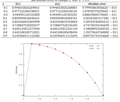
Table-𝟒: Numerical solution using tenth degree spline approximation s(x), exact solution u(x) and absolute errors of example2 with ℎ = 0.1

x S(x) u(x) Absolute error

0.1 0.994653826269063 0.994653826268083 9.7999386383662𝐸 −013

0.2 0.977122206538923 0.977122206528136 1.0787037929560𝐸 −011

0.3 0.944901165332005 0.944901165303202 2.8802960017060𝐸 −011

0.4 0.895094818630416 0.895094818584762 4.5654258151728𝐸 −011

0.5 0.824360635403098 0.824360635350064 5.3034354685621𝐸 −011

0.6 0.728847520203677 0.728847520156204 4.7473025510669𝐸 −011

0.7 0.604125812272944 0.604125812241143 3.1800895250455𝐸 −011

0.8 0.445108185712051 0.445108185698494 1.3557044376000𝐸 −011

0.9 0.245960311116585 0.245960311115695 8.8973273193460𝐸 −013

Figure-𝟒: Comparison of approximate solution and exact solution for example 2withℎ= 0.1

4. COMPARATIVE STUDY OF TENTH DEGREE WITH EIGHTH AND NINTH DEGREE SPLINE FUNCTIONS

Table-5: Comparison of absolute errors for example 1 at h = 0.2

x Exact solution Absolute error Absolute error Absolute error

for 8𝑡ℎdegree[10] for 9𝑡ℎdegree [11] for 10𝑡ℎdegree

0.2 0.195424441305627 5.000000𝑒 −08 3.74400𝑒 −09 6.7174626972𝑒 −011

0.4 0.358037927433905 4.016999𝑒 −07 3.36110𝑒 −08 5.5300902746𝑒 −010 0.6 0.437308512093722 6.220000𝑒 −07 7.56990𝑒 −08 8.44720016158𝑒 −010 0.8 0.356086548558795 2.538000𝑒 −07 6.03450𝑒 −08 3.37260996908𝑒 −010

Figure-𝟓:Comparison of absolute errors for example 1 at h = 0.2

Table-6: Comparison of absolute errors for example 1 at ℎ = 0.1

x Exact solution Absolute error Absolute error Absolute error for 8thdegree[10] for 9thdegree[11] for 10thdegree

0.1 0.09946538262 7.9999𝐸 −08 3.3200𝐸 −10 9.02899977𝐸 −012 0.2 0.19542444130 9.8000𝐸 −07 3.5540𝐸 −09 8.73660033𝐸 −011 0.3 0.283470349 2.3657𝐸 −05 1.2366𝐸 −08 2.523199982𝐸 −010 0.4 0.358037927 7.4400𝐸 −06 2.7224𝐸 −08 4.495109839𝐸 −010 0.5 0.412180317 1.1289𝐸 −05 4.3750𝐸 −08 6.189089796𝐸 −010 0.6 0.437308512 1.3459𝐸 −05 5.4648𝐸 −08 7.258549872𝐸 −010 0.7 0.422888068 1.4430𝐸 −05 5.1837𝐸 −08 7.663260026𝐸 −010 0.8 0.356086547 2.0369𝐸 −05 3.3095𝐸 −08 7.721850381𝐸 −010 0.9 0.221364280 4.7770𝐸 −05 8.5130𝐸 −09 7.825710079𝐸 −010

Table-7: Comparison of absolute errors for example2 at ℎ = 0.2

x Exact solution Absolute error Absolute error Absolute error

for 8𝑡ℎdegree[10] for 9𝑡ℎdegree[12] for 10𝑡ℎdegree

0.2 0.9771222 1.2000𝐸 −08 8.6590𝐸 −09 7.0653483𝐸 −012

0.4 0.89509481 8.6000𝐸 −08 8.3135𝐸 −08 5.47620837𝐸 −011

0.6 0.72884752 1.8500𝐸 −06 1.8903𝐸 −07 8.20919998𝐸 −011

0.8 0.44510818 2.0500𝐸 −06 1.6752𝐸 −07 3.24509863𝐸 −011

Figure-𝟕:Comparison of absolute errors for example2 at ℎ = 0.2

Table-8: Comparison of absolute errors for example2 at ℎ = 0.2

x Exact solution Absolute error Absolute error Absolute error for 8thdegree [10] for 9thdegree[1 for 10thdegree

0.1 0.99465382 7.99990𝐸 −09 9.000𝐸 −10 9.79993863𝐸 −013

0.2 0.97712220 7.87990𝐸 −08 1.410𝐸 −10 1.07870379𝐸 −011

0.3 0.944901165 2.32699𝐸 −07 4.871𝐸 −10 2.88029600𝐸 −011

0.4 0.89509481 3.85500𝐸 −07 3.937𝐸 −09 4.56542581𝐸 −011

0.5 0.82436063 4.10000𝐸 −07 9.280𝐸 −10 5.30343546𝐸 −011

0.6 0.72884752 1.03900𝐸 −07 5.709𝐸 −09 4.74730255𝐸 −011

0.7 0.60412581 3.87499𝐸 −0.7 6.239𝐸 −08 3.1800895𝐸 −011

0.8 0.44510818 8.12699𝐸 −07 1.298𝐸 −08 1.35570443𝐸 −011

0.9 0.24596031 7.56099𝐸 −07 1.048𝐸 −08 8.89732731𝐸 −013

5. CONCLUSION

In this paper we developed the numerical method to obtain the solution of seventh order linear boundary value problems using tenth degree spline. Tenth degree spline approximation has been employed on two problems at different

step lengths. Numerical solution of the problems has been found with ℎ= 0.2 andℎ= 0.1. Computational work has

been carried out using MATLAB software. Approximate solution, exact solution and absolute errors with ℎ= 0.2

and ℎ= 0.1 of the example 1 and example 2 are summarized in Table 1, Table 2, Table 3 and Table 4 respectively. The comparison has been shown in Figures 1, 2, 3 and 4 respectively.

The maximum absolute errors at these step length are 6.7174 × 10−11 and 9.0289 × 10−12 for example 1 at ℎ= 0.2

and ℎ= 0.1 and 7.06534 × 10−12, and 9.79993 × 10−13 for example 2 at ℎ= 0.2 and ℎ= 0.1 respectively. From this we understand that there is good agreement with the exact solution. It is also observed that the approximate solution is more close to the exact solution when h is small. Presented method is compared with the eighth and ninth degree spline approximation [10, 11] at different step lengths. It may be noted from Tables that the presented method is more efficient.

It is observed that the absolute errors are better than the methods in [10, 11]. It is also observed that our proposed method is well suited for the solution of higher order boundary value problems and reduces the computational work. Spline approximations converge to exact solutions more rapidly as the degree increases, if the step length decreases the numerical solution is more accurate.

REFERENCES

1. Akram, G. and H. Rehman, 2011.Solution of fifth order boundary value problems in reproducing

kernel space. Middle-East J. Sci. Res., 10(2): 191-195.

2. Akram, G. and S.S. Siddiqi, 2012.Solution of seventh order boundary value problem using octic spline. Arch.

Des Sci., 65(1), Accepted for Publication (In Press).

3. Ascher, U. M., Mattheij, R. M. M., and Russell, R. D.Numerical solution of boundary value problems for

ordinary differential equations, vol. 13 of Classics in Applied Mathematics. Society for Industrial and Applied Mathematics (SIAM), Philadelphia, PA, 1995. Corrected reprint of the 1988 original.

4. F. Haq, S. Islam, S.I.A.Tirmizi (2009): Numerical solution of boundary-value and initial Boundary-value

problems using spline functions pp1-16

5. I. J. Schoenberg (1946): Contributions to the problems of approximation of equidistant data by analytic

functions. Quart. Appl. Math. 4, 45-99 and 112-141.

6. I. J. Schoenberg (1958): Spline functions, convex curves and mechanical quadrature. Bull. Am. Math. Soc.

64, 352-357.

7. J. H. Ahlberg, E. N. Nilson (1963): Convergence properties of the spline fit. SIAM Journal 11, 95-104.

8. J.Rashidina, M.Khazaei, H.Nikmarvani (2015), Spline collocation method for solution of higher order linear

boundary value problems TWMS. Pure Appl. Math., V.6, N.1, pp 38-47

9. Mohyud-Din, S.T., M.A. Noor and A. Waheed, 2009.Variation of parameters method for solving sixth-order

boundary value problems. Comm.Korean Math. Soc., 24(4): 605-615.

10. P.Kalyani, and Mihretu.N, Eighth Degree spline for seventh order boundary value problems. Journal of

Multidisciplinary Engineering science and Technology (JMEST), ISSN: 3159-0040, V0l.2Issue5, may-2015

11. P. Kalyani and M.N. Lemma, solutions of seventh order boundary value problems using ninth degree spline

functions and comparison with eighth degree spline solutions, Journal of applied Mathematics and physics, 2016, 4, 249-261.

12. Richards, G. and P.R.R. Sarma, 1994. Reduced order models for induction motors with two rotor Circuits.

IEEE Trans. Energ. Conv., 9(4): 673-678.

13. Siddiqi, S.S. and G. Akram, 2006a, b. Solutions of fifth and sixth order boundary-value problems using

nonpolynomial spline technique. Appl. Math. Comput. 175(2): 1574-1581.

14. S. S. Sastry (1976): Finite-difference approximations to one dimensional parabolic equations using cubic

spline technique. J. Comput. Appl. Math. 2, 23-26.

15. Chandrasekhar, S., (1961), Hydrodynamic and Hydromagnetic Stability, Clarendon Press, Oxford, Reprinted:

Dover Books, New York.

16. Bickely, W.G. (1968) Piecewise Cubic Interpolation and Two-Point Boundary Value Problem. Computer

Journal, 11, 202-208.

Source of support: Nil, Conflict of interest: None Declared.