Completely packed O(
n
) loop models and their relation with exactly solved coloring models
Yougang Wang,1Wenan Guo,2,3,*and Henk W. J. Bl¨ote1
1Lorentz Institute, Leiden University, P.O. Box 9506, 2300 RA Leiden, The Netherlands 2Physics Department, Beijing Normal University, Beijing 100875, People’s Republic of China 3State Key Laboratory of Theoretical Physics, Institute of Theoretical Physics, Chinese Academy of Sciences,
Beijing 100190, People’s Republic of China (Received 1 November 2014; published 16 March 2015)
We investigate the completely packed O(n) loop model on the square lattice, and its generalization to an Eulerian graph model, which follows by including cubic vertices which connect the four incoming loop segments. This model includes crossing bonds as well. Our study was inspired by existing exact solutions of the so-called coloring model due to Schultz and Perk [Phys. Rev. Lett.46,629(1981)], which is shown to be equivalent with our generalized loop model. We explore the physical properties and the phase diagram of this model by means of transfer-matrix calculations and finite-size scaling. The exact results, which include seven one-dimensional branches in the parameter space of our generalized loop model, are compared to our numerical results. The results for the phase behavior also extend to parts of the parameter space beyond the exactly solved subspaces. One of the exactly solved branches describes the case of nonintersecting loops and was already known to correspond with the ordering transition of the Potts model. Another exactly solved branch, describing a model with nonintersecting loops and cubic vertices, corresponds with a first-order, Ising-like phase transition forn >2. For 1< n <2, this branch is interpreted in terms of a low-temperature O(n) phase with corner-cubic anisotropy. Forn >2 this branch is the locus of a first-order phase boundary between a phase with a hard-square, lattice-gas-like ordering and a phase dominated by cubic vertices. A mean-field argument explains the first-order nature of this transition. DOI:10.1103/PhysRevE.91.032123 PACS number(s): 05.50.+q,64.60.Cn,64.60.De,75.10.Hk
I. INTRODUCTION
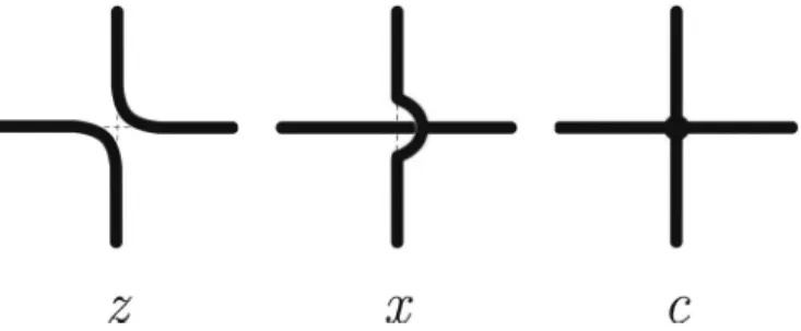
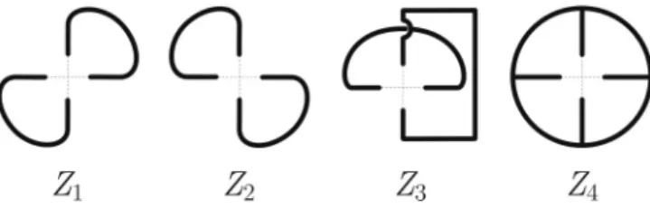
Several types of nonintersecting O(n) loop models can be obtained as a result of an exact transformation of certain O(n )-symmetric spin models [1–6]. Most of these models are two dimensional, but the transformation is also applicable in three dimensions [7]. It provides a generalization of the O(n) model to noninteger and even negative values ofn. Whereas most existing work is restricted to nonintersecting loop models, the models can readily be generalized to include cubic vertices [8] and crossing bonds [9]. These cubic vertices connect to four in-coming loop segments and arise naturally when the O(n) sym-metry of the original spin model is broken by interactions of a cubic symmetry [10]. The crossing-bond vertices occur in the loop representation of nonplanar O(n)-symmetric spin models. The presently investigated model is defined in terms of these three types of vertices on the square lattice. The three types, which are shown in Fig.1together with their vertex weights, specify a complete covering of the lattice edges. In comparison with a recent investigation [11] of crossover phenomena in a densely packed phase of the O(n) loop model, the present set of vertices is obtained by excluding those that do not cover all lattice edges. Due to the absence of empty edges, the physical interpretation in terms of an O(n) spin model is more remote. A formal mapping of the loop model on the spin model leads to a spin-spin interaction energy that can assume complex values when the relative weight of empty edges becomes sufficiently small. However, the mapping of the completely packed O(n) loop model on a dilute O(n−1) loop model model (which was, as far as we know, first formulated by Bl¨ote and Nienhuis; see Ref. [4]) brings it again closer to the realm of the spin models.
*Corresponding author: [email protected]
A configuration of the vertices of Fig.1forms a so-called Eulerian graph G, in which only even numbers of loop segments are connected at each vertex. The present model may thus be called a completely packed Eulerian graph model. The partition sum of this model is
ZEG=
G
zNzcNcxNxnNn. (1)
The sum on G is on all compatible vertex coverings. The exponentsNz,Nc, andNxare the numbers of vertices of types
z,c, andx, respectively, andNnis the number of components
of the graphG. A component is a subset of edges connected by a percolating path of bonds formed by the vertices ofG. Since ZEG is a homogeneous function of the vertex weights, one may, without loss of generality, scale out one of the weights. We thus normalize the weightzof the O(n) vertex describing colliding loop segments to 1.
At this point it is appropriate to comment on our nomen-clature. By “nonintersecting loops” we mean configurations consisting of the type-z vertices in Fig. 1. Since the word “intersecting” could be associated with the type-xvertices, as well as the type-cvertices in Fig.1, we refer to type-xvertices as crossing bonds and to type-cvertices as cubic vertices. Thus, we may, alternatively, call this model a completely packed loop model with crossing bonds and cubic vertices, or just a generalized loop model. Furthermore, we note that the name “fully packed” is used for models where all vertices are visited, but not all edges are covered by loop segments [12,13].
FIG. 1. The vertices of the completely packed O(n) loop model with crossing bonds and cubic vertices on the square lattice, together with their weights. Fourfold rotational symmetry of the model requires that the weights for the two possible orientations of the z-type vertex are the same.
in such a way that, for any given color, an even number of edges connects to each vertex. Exact solutions were found for several different branches of critical lines that are parametrized by the number of colors. Our purpose is to put them in the broader context of statistical physics by exploring the universal properties and phase behavior at and near their intersections with the phase diagram spanned by the parameters in Eq. (1). The outline of this paper is as follows. In Sec. II we reformulate the Eulerian graph model in terms of the number of loops and describe the transformation connecting it to the coloring model. We review the exact results for the free energy, which apply to several one-dimensional “branches” parametrized by n in the parameter space of Eq. (1) and which are useful for the analysis of the conformal anomaly along these branches. This analysis is based on transfer-matrix calculations, for which some technical details are provided in Sec.IIIand the Appendix. Results for the free energy of the exactly solved branches are presented in Sec.IVand for some scaling dimensions in Sec. V. While the exploration of the complete (in fact three-dimensional) phase diagram of Eq. (1) is beyond the scope of the present paper, the embedding of some of the exactly solved branches in this diagram is investigated in Sec. VI. Our conclusions are presented and discussed in Sec.VII.
II. MAPPINGS AND EXISTING THEORY A. Euler’s theorem
Euler’s theorem specifies that the number of components satisfiesNn=Ns−Nb+Nl, whereNsis the number of sites
of the lattice,Nb is the number of bonds covered byG, and
Nl is the number of loops in G. It means that every new
bond decreasesNnby one, unless its end points were already
connected. Application of this theorem to the present model requires some care because it merges the degrees of freedom of the cubic model with those of the O(n) model. Whereas the spins of the cubic model [8,19] are defined on the vertices of the square lattice, those of the square-lattice O(n) model [4,5] sit in the middle of the edges. Here we adopt the definition for the square-lattice O(n) loop model. Thus, the numberNs
of sites in Euler’s relation becomes twice the number Nv
of vertices. Furthermore, in this formulation, a cubic vertex consists ofthree bonds: It connects one pair of sites along the x direction and one pair of sites along the y direction,
and it also makes a connection between both pairs. Thus, for the present model, the number of bonds as required in Euler’s formula isNb=2Nz+2Nx+3Nc, and Euler’s theorem takes
the form
Nn=Ns−2Nz−2Nx−3Nc+Nl=Nl−Nc, (2)
where the last step usesNs=2Nv andNv=Nz+Nx+Nc
in the completely packed model. After substitution of Euler’s theorem, the partition sum Eq. (1) is thus reformulated as
ZEG=Zloop=
G
zNz(c/n)NcxNxnNl. (3)
The Boltzmann weights now only depend on the numbers of vertices of each type and on the number of loops. This formula exposes the nature of the partition sum as that of a generalized loop model: The numberNnof components is now absent, and
the weight of a cubic vertex now appears ascn≡c/ninstead
of c. In this context it is noteworthy that the cubic weightc used in Ref. [11] is equal tocn=c/nwhen expressed in the
parameters of the present work.
B. Relation with the coloring model
The Perk-Schultz coloring model is defined in Refs. [14,15] in terms of bond variables that can assumendifferent colors. The colors of the bonds connected to a given vertex are not independent. The number of bonds of a given color connected to a vertex is restricted to be even. Following Ref. [14], the vertex weights are denoted Rλμ(αβ), where λ,μdenote the
colors of the bonds in the−x,+x directions andα,β apply to the−y,+y directions, respectively. The color restrictions and symmetries are expressed by
Rλμ(αβ)=Wαλd δαβδλμ+Wαβr δαλδβμ+Wαβl δαμδβλ, (4)
with
Wαβr =Wr(1−δαβ), Wαβl =Wl(1−δαβ), (5)
and
Wαβd =Wdδαβ+W0(1−δαβ). (6)
The weights thus satisfy the color permutation symmetry. We furthermore impose the symmetry condition
Wl=Wr, (7)
which leads to vertex weights that are invariant under rotations by π/2, thus allowing conformal symmetry of the coloring model in the scaling limit.
The model still contains, besides the numbernof colors, three variable parametersW0,Wd, andWr. The partition sum of the coloring model is defined by
Zcm=
C
v
Rλvμv(α
vβv), (8)
where the sum onCis over all colors of each bond and the prod-uct is over all verticesv. Each bond variable occurs twice in the product, once as a superscript and once as an argument ofR.
FIG. 2. The four different ways in which the incoming bonds at a vertex can be connected by the remaining configuration of the generalized loop model. The corresponding restricted partition sums are indicated under the figures.
coloring model [21] and the model of Eq. (3). This follows simply by the interpretation of the weightnof each component in Eq. (1) in terms of a summation onndifferent colors. Then the set of configurations of the loop model precisely matches that of the coloring model with weights according to Eqs. (4)– (6). The relation of the parametersWd,W0, andWr withz, x, andcfollows by matching the partition sums as expressed in the two types of vertex weights. After removing one vertex fromG, the connectivity of the incoming bonds, as determined by the surrounding loop model configuration, is denoted by an integer 1–4, specified in Fig.2. The corresponding restricted partition sums of the generalized loop model are denoted asZ1 toZ4. They do not yet include the degeneracy factornof the incomplete loops connected to the incoming bonds. In terms of these restricted sums and the local vertex weights of the coloring model, the partition sum is obtained by summation on the color combinations allowed by the diagrams in Fig.2as
Zcm=[(n2−n)Wr+nWd](Z1+Z2)
+[(n2−n)W0+nWd]Z3+nWdZ4. (9)
Using instead the local vertex weights of the generalized loop model, the partition sum follows, taking into account the weightnper component specified by Eq. (1), as
Zloop=[(n2+n)z+nx+nc](Z1+Z2)
+n(2z+nx+c)Z3+n(2z+x+c)Z4. (10) The equivalence of both models requires that the prefactors of Z1+Z2, Z3, and Z4 are the same in both forms of the partition sum. These conditions lead to three equations, whose solution shows that the models are equivalent for
W0=x
Wd=2z+x+c
Wr =z
⎫ ⎬
⎭. (11)
In the representation of Eq. (1), the parameterndescribing the number of colors is no longer restricted to positive integers.
C. The branches resulting from the solution of the coloring model
Several cases of the coloring model were studied analyti-cally by Schultz [14]. That work provided analytic expressions for the partition sum per site. Included are results for a number of index-independent models, i.e., models satisfying Eqs. (4)–(6), so that all colors are equivalent. As noted above, the present work also restricts the vertex weight to be invariant
TABLE I. Intersection between the exactly solved subspaces of the coloring model and the parameter space of the generalized loop model. These intersections form seven branches, defined in the first column, for which we also include the vertex weights. The entries under “Case” show the labeling used by Schultz [14], with the characters “a” and “b” appended in order to separate the Schultz cases into branches with single-valued vertex weights.
Vertex weights
Branch Case z x c
1 IIA1 1 0 0
2 IIA2a 1 0 −1+√n−1
3 IIA2b 1 0 −1−√n−1
4 IIB1a 1 2−4n 0
5 IIB1b 1 n−2
4
2−n
2
6 IIB2a 0 1 0
7 IIB2b 0 1 −2
under rotations byπ/2, as required by asymptotic conformal invariance [22]. This enables the numerical estimation of some universal quantities as outlined in Sec.III.
After application of these restrictions, the cases studied by Schultz reduce to seven one-dimensional subspaces in the parameter space of the loop model. These correspond, according to Eq. (11), with exactly solved “branches” of the generalized loop model of Eqs. (1) and (3). The vertex weights are shown in TableIas functions ofnfor these seven branches. These weights are normalized such that z=1, except for branches 6 and 7, where z vanishes, and we normalize as x =1 instead.
1. Branch 1
The exact solution of branch 1 by Schultz [14] is presented in terms of a quantity denoted there as f, which matches the per-site partition function, with the normalizationWd= 1 [15]. Branch 1 has nonzero weights only for colliding vertices of theztype, as shown in Fig.1. It thus applies to a completely packed, nonintersecting loop model. For n0, this branch is exactly equivalent with the six-vertex model and with the q =n2-state Potts model at its transition point [23]. Due to these equivalences, much is already known for branch 1. We recall some of these results for reasons of completeness as well as relevance for the interpretation of the phase diagram of Eq. (1).
Exact solutions of the aforementioned equivalent models were already given by Lieb [24] and Baxter [25], respectively. After taking into account the different normalizations of the vertices, and the fact that the number of Potts sites is one half of the number of vertices, the Schultz result for the free energy per vertex in the rangen >2 has been shown [26] to agree with the results of Lieb and Baxter in the corresponding parameter range. The Schultz result does not apply forn2, but there various other results for the free energy [24–28] are available. In the thermodynamic limit, the following results for the free energy per vertex apply:
f(n)= 1 2θ+
∞
k=1
exp(−kθ) tanh(kθ)
withθdefined by coshθ=n/2;
f(2)=2 ln (1/4)
2(3/4), (13)
f(n)= 1 2
∞
−∞
dxtanhμx sinh(π−μ)x
xsinhπ x , (−2< n <2),
(14)
where the parameterμis defined byμ≡arccos(n/2);
f(−2)=0, (15)
f(n)= 1 2θ˜+
∞
k=1
[−exp(−θ˜)]k tanh(kθ˜)
k , (n <−2),
(16)
where cosh ˜θ = −n/2. The expression forn <−2 applies [26] to the thermodynamic limit of a system with a number of vertices equal to a multiple of 4.
The correlation functions are known to follow a power law as a function of distance in the critical range−2n2 and to decay exponentially for|n|>2. The off-critical phase for largenis known [26] to display the same type of order as the square lattice gas with nearest-neighbor exclusion.
2. Branches 2 and 3
These branches contain both colliding (ztype) and cubic vertices (c type), as shown in Fig. 1, with a weight that depends on n. Their nature differs from branch 1 in the fact that different loops may now have common edges and vertices and thus be forced into the same component, according to Eq. (1).
In order to avoid confusion with our notation, we denote the Schultz result for the per-site partition function aszS, instead of
f as used there, which we reserve for the free-energy density. After substitution of the parameters as determined by Eq. (11) and TableIinto the result [14] forzSof branches 2 and 3 and some simplification, the free-energy per vertex follows as
f =ln(WdzS)
=ln
n−1
|−1±√n−1| ∞
k=1
1∓(n−1)−2k−1/2 1∓(n−1)−2k−3/2
2
,
(17)
where the upper signs in ± and ∓ apply to branch 2 and the lower signs apply to branch 3. This result applies to the thermodynamic limit of systems with an even number of vertices. Its validity cannot extend into the rangen <2, since the infinite product vanishes there. Forn→2, branch 2, the infinite product compensates the divergence of the prefactor. Since branch 2 intersects with branch 1 atn=2, its free energy atn=2 is given by Eq. (13). For branch 3, the infinite product assumes the value 2 in the limitn→2, so that the free energy vanishes in this limit.
3. Branches 4 and 5
For branch 4, the system contains, in addition to the z-type colliding vertices, also x-type crossing-bond vertices
(see Fig. 1), but no cubic vertices. A problem arises with the free-energy density corresponding with subcase IIB1 of Ref. [14], since it displays many divergences as a function of n. Furthermore, footnote [64] of Ref. [15], which applies to this result in Ref. [14], allows for the possibility that this result has to be modified by an additional factor. In order to determine this factor, we focus on the quantity zS as given by Schultz [14]. In the present parameter subspace, it reduces to
zS(n)= 2−n
4 21
4
23 4
1 2 +α
(1−α)
12 −α(α) , α≡ 6−n 4(2−n).
(18)
After two applications of Euler’s reflection formula, one finds
zS(n)= 2−n
4
214
23 4
2
α+12
2(α) ctg(απ). (19)
An independent calculation of the exact free-energy density of branch 4 is due to Rietman [29]. That result was derived for the intersecting loop representation in Eq. (3), whose relation with the coloring model was not immediately obvious. The Rietman expression for the free energy is free of divergences for n <2. Numerical evaluation shows that, although the Schultz and Rietman results are different, they differ only by a fractional number for some fractional values ofn. We thus cast the Rietman resultzRfor the per-site partition function in a similar form as Eq. (19). It is [29]
zR(n)=
4κ 1+κu(1−u)
×
1+u232−u212+21κ +u21+21κ −u2 1
2+
u
2
1−u21
2κ + u
2
1
2+ 1 2κ −
u
2 ,
(20)
where κ ≡1−n2, and u describes the anisotropy of the model when the twoz-type colliding vertices have different weights, sayz1andz2asu=z1/(z1+z2); in our work,u= 12. Substitution ofκ anduin Eq. (20) leads to
zR(n)=16 2−n 10−n
25 4
23 4
23n−10 4(n−2)
2 n−6 4(n−2)
= 2−n
10−n 21
4
23 4
2(α+ 1 2)
2(α) , (21)
where the last equality uses the definition (18) of α. A comparison of Eqs. (19) and (21) shows that
zS(n)= 10−n
2−n ctg(απ)zR(n). (22)
density of branch 4 follows, in our normalizationz=1, as
f(n)=ln 10−n 4 zR
=ln
2−n
4
214
23 4
2
α+12
2(α)
.
(23)
This expression is well behaved forn <2, but in the range 2< n <6 it does not exhibit the expected type of behavior, because the arguments of the functions can diverge and become negative. The fact that branches 1 and 4 intersect at n=2 allows a consistency check by taking the limitn→2 in Eq. (23). Since α diverges, we may safely apply Stirling’s formula. It then follows that the ratio of the divergent functions just cancels the prefactor 2−n, so that we indeed reproduce Eq. (13).
The vertex weights for branch 5 differ from branch 4 in the additional presence ofc-type cubic vertices. The Schultz result [14] for branch 5 specifies the same expression for the partition function as for branch 4. Later we compare our numerical results for branches 4 and 5 with Eq. (23) for several values ofn.
4. Branches 6 and 7
The vertex weights of branches 6 and 7, given in TableI, do not depend onn, but the partition sum still contains the loop
weight explicitly, and indeed it appears in the exact per-site partition sumzSas given by Schultz [14]. This result leads to the free-energy density
f(n)=ln[zS]=ln
nb11+(nnb−2)b
1nb−b1+(nnb−1)b
, (24)
where
b= W
r
Wd =
z
2z+x+c =0.
Since we impose rotational symmetry overπ/2 on the vertex weights by Eq. (7), and moreoverWlWr=0 for branches 6 and 7, we arrive at the special pointb=Wr=z=0. We thus take the limitb→0 in Eq. (24):
f(n)=lim
b→0
ln
1 nb
+ln 1+(n−2)b
nb
− ln
1−b
nb
−ln 1+(n−1)b
nb
. (25)
Each of the arguments of thefunctions diverges in the limit ofb=0. We apply Stirling’s formula and neglect terms that vanish in this limit:
f(n)=lim
b→0
2−nb
2nb [−ln(nb)]− 1 nb+
1 2ln(2π)
+
2+nb−4b
2nb {ln[1+(n−2)b]−ln(nb)} −
1+(n−2)b
nb +
1 2ln(2π)
−
2−nb−2b
2nb [ln(1−b)−ln(nb)]− 1−b
nb +
1 2ln(2π)
−
2+nb−2b
2nb {ln[1+(n−1)b]−ln(nb)} −
1+(n−1)b
nb +
1 2ln(2π)
.
We first consider the divergent terms with ln(nb). The sum of their amplitudes is seen to cancel exactly:
2−nb 2nb +
2+nb−4b
2nb −
2−nb−2b
2nb −
2+nb−2b 2nb =0.
Similarly, the sums of the amplitudes of terms with 1
nb and
1
2ln(2π) vanish. Therefore,
f(n)=lim
b→0
2+nb−4b
2nb ln[1+(n−2)b]
− 2−nb−2b
2nb ln(1−b)
− 2+nb−2b
2nb ln[1+(n−1)b]
.
The prefactors depend linearly on 1/b, and the logarithms are proportional tob in lowest order. It is therefore sufficient to keep the divergent part of the prefactors and the terms withb
in the logarithms:
f(n)=lim
b→0
1
nb[(n−2)b+b−(n−1)b]
=0. (26)
Thus, according to the Schultz solution, the free-energy density of branches 6 and 7 vanishes in the thermodynamic limit
L→ ∞.
D. Exact results for the scaling dimensions and conformal anomaly
1. Results for branch 1
gas results given below and with an exact analysis of the model on the square lattice [31,32].
The Coulomb gas method, which offers a way to calculate some scaling dimensions, was explained in some detail in Ref. [10]. It considers an observable local density p(r) on positionr, which depends on the microstate at positionrand is conjugate to the fieldq. In a critical state, we expect that the two-point correlation behaves asp(0)p(r) ∝r−2Xq, where
the exponentXqis the scaling dimension of the densityp. Via
the relation with the Coulomb gas one may now associatep(0) with a pair of charges, an electric chargee0, and a magnetic onem0. Similarly, we have a pair er,mr representing p(r).
Then, the scaling dimensionXq is given by [10]
Xq =X(e,m)= −
e0er
2g − m0mrg
2 . (27)
The Coulomb gas couplinggmay be obtained if some exact information about the universal properties is available. Its determination, as well as that of the electric and magnetic charges, is a technical problem that we leave aside. We copy their values from the literature and present only the result in terms ofXq when needed.
For the critical O(n) model, as well as for its analytic continuation into the low-temperature O(n) phase, it is well established how to apply the Coulomb gas method [10]. In particular, the low-temperature O(n) phase, which shares its universal properties with the completely packed O(n) loop model of branch 1, is important for the present research. The Coulomb gas results include the following scaling dimensions of the critical O(n) model and the low-temperature phase:
Xh=1−
3g 8 −
1
2g, Xt = 4
g−2, (28)
where Xt is the leading temperature dimension of the O(n)
model. The Coulomb gas coupling constantgis given by
g=1± 1 π arccos
n
2, (29)
where the+sign applies to the critical O(n) model and the
− sign to the dense low-temperature phase corresponding with branch 1. Furthermore, the introduction of thex- and c-type vertices into the nonintersecting O(n) loop model can be analyzed using the Coulomb gas [10,33]. These perturbations are described by the cubic-crossover exponent
Xc(g)=1+
3g 2 −
1
2g. (30)
This perturbation is relevant in the dense phase, thus crossing bonds and cubic vertices are expected to lead to different universal behavior in the range−2< n <2.
Next we express the conformal anomalycaas a function of the coupling constantg. From the definition of the parameter yas a function ofnin Ref. [34], one finds that it relates tog byy=2−2gin our notation. Then, using Eqs. (1) and (9) of Ref. [34], one obtains the conformal anomaly as
ca(g)=13−6g− 6
g. (31)
2. Results for the other branches
As far as we are aware, no exact results are available for the universal parameters of branches 2 and 3 and equivalent models. However, as mentioned in the preceding section, the cubic perturbation, i.e., the vertex weight c, is expected to introduce new universal behavior for branches 2 and 3 with respect to branch 1. Numerical results [11] for the dense phase (not completely packed) of the model with z- and c-type vertices confirm this and show the existence of a phase with a small value of the magnetic dimensionXh, i.e., a phase in
which magnetic correlations persist over long distances. The same Coulomb gas result applies to the introduction of crossing bonds, which is, like the cubic perturbation, also described by the four-leg watermelon diagram, and one may thus expect new universal behavior for branch 4. A few results are available for a supersymmetric spin chain [9] related to branch 4, referred to as the Brauer model [35,36]. Numerical as well as analytical arguments support, forn2, the formula for the conformal anomaly
ca(n)=n−1, (n2), (32)
and the magnetic dimensionXhis reported to be very small,
suggesting anomalously slow decay of magnetic correlations, at least for n=1. This behavior was confirmed, although with limited accuracy, for a densely packed O(n) model with crossing bonds, which is believed to display similar universal behavior as branch 4 [11]. This model was also studied by Jacobsen et al. [37], and recently, correlation functions were obtained by Nahumet al.[38] forn <2, decaying as an inverse power of the logarithm of the distance. As far as universal behavior is concerned, these findings for the completely packed model apply as well in the dense O(n) phase, but not for the O(n) transition to the high-temperature phase, where the cubic perturbation is irrelevant for|n|<2. The latter point was numerically confirmed for then=0 [39] case, which describes intersecting trails.
III. TRANSFER-MATRIX METHOD
We use the transfer-matrix method to calculate the partition sumZof a square lattice model, wrapped on the surface of a cylinder with a circumference ofLlattice units. The cylinder may be infinitely long but its circumference L is finite. We postpone the transfer-matrix construction to the Appendix. Here we focus on the calculation of the free energy, the conformal anomaly and the scaling dimensions, which define the universality class. A finite-size analysis of the free energy does not only yield the conformal anomaly, but a comparison with the exact free energy, if available, provides a useful consistency check.
Free energy and correlation lengths
0(L) as
f(L)=L−1ln0(L). (33)
The transfer-matrix results forf(L) can be used to estimate the conformal anomalycausing the relation [34,41]
f(L)f + π ca
6L2. (34)
The subdominant eigenvalues k(L) of T determine the
correlation lengthsξkbelonging to thekth correlation function.
The gap with respect to the largest eigenvalue determines the corresponding correlation length along the cylinder as
ξk−1(L)=ln 0
|k|, (35)
where it is usual to associate the labelk=1 with the magnetic correlation length ξm and k=2 with the energy-energy
correlation lengthξt. For the purpose of numerical analysis, it
is convenient to define the corresponding scaled gapsXk(L) as
Xk(L)=
L 2π ξk(L)
. (36)
In the presence of a temperature fieldt and an irrelevant field u, its scaling behavior is
Xk(t,u,L)Xk+aLytt+bLyuu+ · · · , (37)
whereXk is the scaling dimension of the observable whose
correlation length is described by ξk [42]. This formula
provides a basis to observe the phase behavior as a function of a parameter, such as a vertex weight, that contributes to t. Ifyt>0 anduis not too large, a set of curves displaying
Xk(L) versus that parameter for several values of the system
sizeLwill show intersections converging to the point where the relevant scaling field t vanishes, i.e., the point where a phase transition occurs. According to Eq. (37), the slopes of theXk(L) curves at the intersections increase withLifyt>0.
In the data analysis, we make use of this criterion for the relevance of the scaling fieldt.
While the calculation of the temperaturelike scaling dimen-sionX2=Xtfrom2is straightforward, that of the magnetic dimension Xh needs further comment. In the loop model,
magnetic correlations between O(n) spins are represented by a single loop segment between the two sites. In completely packed models, it is not possible to add another loop segment into the system, and we use a method employed, e.g., in Ref. [11]. It analyzes the difference between the leading eigenvalues of systems with odd system sizeLcontaining such a segment and even systems without such a segment. Thus, one defines scaled gaps using the average of two consecutive even (or odd) systems as
Xh(evenL)=
L 2π
ln0(L)− 1
2[ln|1(L−1)|
+ln|1(L+1)|]
,
or (38)
Xh(oddL)=
L 2π
1
2[ln|0(L−1)| +ln|0(L+1)|]
−ln1(L)
,
where1denotes the largest eigenvalue of odd systems in the transfer-matrix sector that includes an odd segment.
IV. NUMERICAL RESULTS FOR THE FREE ENERGY This section presents the finite-size analysis of the transfer-matrix results for the free energy of the seven branches following from the Schultz solutions [14] and the mapping on Eqs. (1) and (3). The vertex weights for these seven branches are listed in TableI.
A. Branch 1
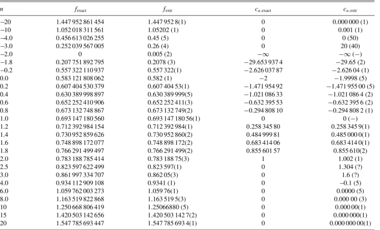
Some numerical results for branch 1 are already listed in Ref. [26], together with an analytic derivation of the free energy for n <−2. Here we summarize those results and provide additional data. The finite-size data for the free energy were extrapolated using Eq. (34), yielding estimates off(n), which are listed in TableII. Forn= −2, the finite-size data for the free energy did not obey Eq. (34), but were, up to numerical precision, precisely proportional to 1/L. Accordingly, we quote the resultsf(−2)=0 and, for the conformal anomaly, ca= −∞. For most values of n, these free energies agree satisfactorily with the theoretical values given in Eqs. (12) to (16). Next, the free energies in Eq. (34) were fixed at their theoretical values, in order to obtain improved estimates of the conformal anomaly. These results are also listed in Table II and appear to agree well with the theoretical values, except for the ranges where|n| slightly exceeds 2 and where poor finite-size convergence occurs.
B. Branches 2 and 3
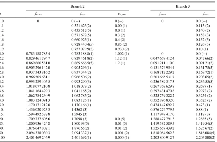
The finite-size data for the free energy of branch 2 were fitted by Eq. (34). Fits with two iteration steps, as described, e.g., in Ref. [40], were employed, using various combinations of exponents that were left free or fixed at expected integer values. A comparison between the different fits, and between fits using even and odd system sizes, thus yielded error estimates. The best estimates off(n) are listed in TableIII.
One observes that the bulk free energy for n >2 is in agreement with the Schultz solution [14]. Since branches 1 and 2 intersect atn=2, we took then=2 exact result for branch 1 in the second column of Table III. Forn=1, branches 2 and 3 are connected and the partition sum allows independent summation on the vertex states, which yields a factor 1 per vertex. This yields the exact resultsf(1)=0 andca=0, also shown in TableIII. Forn=2, branch 3, the largest eigenvalue of the transfer matrix is 2 for all even system sizes; therefore, the bulk free energy and the conformal anomaly also vanish in this case.
While the bulk free energy is well resolved in most cases, complications arise for the part of branch 3 with smalln. The free energy for a small system seems to converge well to a limiting value as
f(n)= ±√n−1+12(n−1)∓53(n−1)3/2+ · · ·, (39)
TABLE II. Fit results for the free-energy density and the conformal anomaly of the branch 1 model, compared with the theoretical values. Estimated numerical uncertainties in the last decimal place are given between parentheses. The entries “0 (−)” indicate that the raw numerical data agree, up to numerical precision, with a vanishing result.
n fexact fextr ca,exact ca,extr
−20 1.447 952 861 454 1.447 952 8(1) 0 0.000 000 (1)
−10 1.052 018 311 561 1.05202 (1) 0 0.001 (1)
−4.0 0.456 613 026 255 0.45 (5) 0 0 (50)
−3.0 0.252 039 567 005 0.26 (4) 0 20 (40)
−2.0 0 0.005 (2) −∞ −∞(−)
−1.8 0.207 751 892 795 0.2078 (3) −29.653 937 4 −29.65 (2)
−0.2 0.557 322 110 937 0.557 322(1) −2.626 037 87 −2.626 04 (1)
0.0 0.583 121 808 062 0.582 (1) −2 −1.9998 (5)
0.2 0.607 404 530 379 0.607 404 53(1) −1.471 954 92 −1.471 955 00 (5)
0.4 0.630 389 998 897 0.630 389 999(5) −1.021 086 33 −1.021 086 4 (2)
0.6 0.652 252 410 906 0.652 252 411(3) −0.632 395 53 −0.632 395 6 (2)
0.8 0.673 132 748 867 0.673 132 749(2) −0.294 808 10 −0.294 808 2 (1)
1.0 0.693 147 180 560 0.693 147 180 56(1) 0 0 (−)
1.2 0.712 392 984 154 0.712 392 984(1) 0.258 345 80 0.258 345 9(1)
1.4 0.730 952 859 626 0.730 952 860(2) 0.484 999 81 0.485 000 0(1)
1.6 0.748 898 172 077 0.748 898 172(2) 0.683 414 06 0.683 414 0(1)
1.8 0.766 291 499 497 0.766 291 499(2) 0.855 601 57 0.855 610(2)
2.0 0.783 188 785 414 0.783 188 75(3) 1 1.002 (1)
2.5 0.823 597 622 499 0.823 597(1) 0 1.304 (?)
3.0 0.861 997 334 707 0.862 05(3) 0 1.6 (?)
4.0 0.934 112 909 108 0.9341 (1) 0 −0.1 (5)
6.0 1.059 762 003 273 1.059 76(1) 0 0.0000 (5)
8.0 1.163 519 822 868 1.163 519 5(3) 0 0.000 00 (3)
10 1.250 668 806 419 1.25066880 (5) 0 0.000 00(1)
15 1.420 503 142 656 1.420 503 142 7(2) 0 0.000 000(1)
20 1.547 785 693 447 1.547 785 693 4(1) 0 0.000 000 00(1)
the range of accessible system sizes. The eigenvalue crossings shift to smallerLfor larger values ofn. Thus, we believe that Eq. (39) does not apply to the bulk free energy of branch 3, not even forn close to 1. In addition to the level crossing, the free-energy data display oscillations with a period 4 in the system size for branch 3. For these reasons the free energies of branch 3 could not be accurately determined in the interval 1< n <2.
The conformal anomaly for branch 2 was estimated by least-squares fits on the basis of Eq. (34), with the finite-size exponent fixed at−2. These fits do not show the type of fast convergence as that of branch 1. Especially for n <2, we observe that strong crossover effects play a role, so that the errors are difficult to estimate. Forn >2, there exists a range of nwhere the numerical results seem to suggest, as indicated in the table, a conformal anomalyca>1, but iterated fits display a diverging trend, which becomes progressively stronger with increasingn. Thus, the entries forcain TableIIIfor 2< n < 2.6 may not be taken too seriously. For largern, the data are no longer suggestive of convergence to a value ofca>0. Only forn20 do we observe the exponential convergence of the free energy withL that is expected in a noncritical phase, corresponding withca=0.
For branch 3, the finite-size data for f are, remarkably, behaving more like f(L)=f(∞)+a/L, which does not suggest a finite conformal anomaly. Forn5, the absolute value of the effective exponent becomes significantly larger than 1 and tends to increase withL, in accordance with the
expected crossover to exponential behavior, which is indeed seen forL25. Convergence is poor in the crossover range aroundn=10, and the extrapolated values of the free energy are relatively inaccurate in that range.
An investigation into how branches 2 and 3 are embedded in thecnversusnphase diagram is reported in Sec.VI.
C. Branch 4
The branch-4 system contains crossing bonds instead of the cubic vertices considered in the preceding section. The largest eigenvalues of the transfer matrix were computed for a number of values of the loop weightnfor system sizes up toL=16. The extrapolated values of the free-energy density forn2 agree accurately with the exact expression given by Eq. (23), as shown in TableIV. That expression does, however, no longer agree with the numerical results listed for the rangen >2.
However, the free-energy data listed in TableIVaccurately display a symmetry with respect to the pointn=2. It is thus straightforward to conjecture an exact expression for the free-energy density along branch 4 for alln, by replacing n−2 with|n−2|in Eq. (23):
f(n)=ln
|n−2| 4
+2 ln
1 4
−2 ln
3 4
−2 ln
1 4+
1
|n−2|
+2 ln
3 4 +
1
|n−2|
.
TABLE III. Numerical results for the free-energy density of the branch 2 and 3 models, compared with the theoretical values. Fit results for the conformal anomaly of branch 2 are also shown. Estimated numerical uncertainties in the last decimal places are given between parentheses. The entries “0 (−)” indicate that the raw numerical data agree, up to numerical precision, with a vanishing result.
Branch 2 Branch 3
n fexact fextr ca,extr fexact fextr
1.0 0 0 (−) 0 (−) 0 0.0 (−)
1.1 0.321 623(2) 0.00 (1) 0.113 (2)
1.2 0.435 512(5) 0.0 (1) 0.140 (2)
1.4 0.571 672(5) 0.3 (2) 0.158 (3)
1.6 0.660 925(1) 0.4 (2) 0.152 (5)
1.8 0.728 440 4(5) 0.85 (2) 0.126 (5)
1.9 0.757 079 9(2) 0.930 (2) 0.10 (1)
2.0 0.783 188 785 4 0.783 188 8(1) 1.002 (1) 0 0.0 (−)
2.2 0.829 461 794 7 0.829 461 8(2) 1.12 (1) 0.047 659 412 4 0.047 66(2)
2.4 0.869 666 581 0 0.869 666 5(5) 1.2 (1) 0.091 211 110 0 0.091 21(2)
2.6 0.905 296 142 0 0.905 296(1) 0.131 374 954 4 0.131 75(5)
2.8 0.937 343 816 2 0.937 344(2) 0.168 712 229 2 0.168 72(1)
3.0 0.966 505 681 1 0.966 506(2) 0.203 665 531 7 0.203 65(2)
3.2 0.993 289 405 5 0.993 290(3) 0.236 589 317 3 0.236 55(5)
3.4 1.018 077 210 8 1.018 078(2) 0.267 768 629 8 0.2677 (1)
3.6 1.041 164 429 3 1.041 165(2) 0.297 431 470 8 0.2972 (2)
3.8 1.062 784 230 9 1.062 785(2) 0.325 759 322 2 0.3254 (2)
4.0 1.083 124 091 3 1.083 125(1) 0.352 896 832 0 0.3525 (2)
5.0 1.170 171 212 8 1.170 166(1) 0.474 147 692 7 0.473 (1)
10. 1.436 020 923 3 1.4362 (3) 0.876 274 779 5 0.88 (1)
15. 1.594 492 588 8 1.5945 (3) 1.117 947 417 0 1.118 (3)
20. 1.709 737 605 6 1.7098 (3) 0.0 (5) 1.288 477 791 3 1.2885 (5)
25. 1.800 936 424 8 1.800 93(5) 0.01 (5) 1.419 532 589 5 1.419 54(5)
30. 1.876 647 802 1 1.876 65(2) 0.01 (2) 1.525 657 439 2 1.525 67(2)
50 2.094 338 030 3 2.094 337(1) 0.001 (2) 1.818 084 562 3 1.818 084(5)
100 2.401 469 246 9 2.401 692(1) 0.000 (1) 2.203 800 912 7 2.203 800(2)
Whereas the bulk free energy displays a clear symmetry with respect to the pointn=2, this is not the case for the finite-size results for the free energy. Accordingly, the estimated values of the conformal anomaly, also included in TableIV, do not obey the symmetry. These estimates ofcawere obtained by fits according to Eq. (34), with the bulk free energy fixed according to Eq. (40). Our confidence in this procedure is based on the degree of accuracy found above for the agreement between the extrapolated values of the free energy and Eq. (40).
In the rangen2, the results for the conformal anomaly are suggestive of behavior according to Eq. (32). While the finite-size dependence of the estimates ofcais quite small, their apparent convergence is very slow in this range. This makes it difficult to estimate the error margins, so that our new evidence supporting Eq. (32) may not be considered as very convincing. The fits forcain the rangen2 are better behaved, and the numerical results in TableIVallow the conjecture
ca=n/2 (n2). (41)
This type of behavior is already strongly suggested by first estimates ofcaas 6π−1L2[f(L)−f(∞)]. Such estimates in the range 3n8 differ less than 10−2fromn/2 forL=16. However, apparent convergence is slow, and we were unable to reduce the estimated uncertainty margins much below the 10−2level by means of iterated fits.
D. Branch 5
The definition of branch 5 specifies that both crossing bonds and cubic vertices occur in addition to the original O(n)-type vertices. In the representation of the coloring model, the vertex weights of branch 5 according to Eq. (11) are equal to those for branch 4, except for a change of sign of the weight W0 describing a color crossing. In an infinite system, such crossings occur in pairs, so that the free-energy density for branch 5 must be equal to that for branch 4. This may be expected to hold also for finite systems with an even system size, which is confirmed by our transfer-matrix results for the largest eigenvalue, at least forn >−2. A level crossing occurs atn= −2, and forn <−2 the largest eigenvalue of a system with a size L divisible by 4 has an eigenvector that is antisymmetric under translations. Such eigenvalues do not contribute to the free energy of a translationally invariant system. For systems with a size equal to an odd multiple of 2, the largest eigenvalues of branch 4 coincide with those of branch 5, also forn <−2.
TABLE IV. Fit results for the bulk free-energy density of branches 4 and 5, compared with the theoretical valuesfRgiven by Rietman [29]. Estimated numerical uncertainties in the last decimal place are given between parentheses. Error margins quoted as “(−)” indicate that the raw finite-size data agree, with a numerical precision determined only by rounding errors, with the listed result. This table is organized such as to display the symmetryf(2+x)=f(2−x) of the free energy. Results for the conformal anomaly, estimated from the finite-size dependence of the free-energy data, are also listed.
n fR fextr ca,extr n fextr ca,extr
2.0 0.783 188 785 414 0.783 190(2) 1.002 (2) 2.0 0.783 190(2) 1.002 (2)
1.6 0.788 072 581 927 0.788 072(2) 0.66 (1) 2.4 0.788 070(4) 1.32 (2)
1.2 0.801 609 709 369 0.801 610(2) 0.22 (1) 2.8 0.801 607(5) 1.40 (1)
1.0 ln(9/4) ln(9/4) (−) 0 (−) 3.0 0.810 929(2) 1.50 (1)
0.8 0.821 583 452 525 0.821 58(1) −0.22 (2) 3.2 0.821 583(1) 1.60 (1)
0.6 0.833 330 017 842 0.833 33(1) −0.44 (3) 3.4 0.833 329(1) 1.70 (1)
0.4 0.845 964 458 726 0.845 96(1) −0.65 (5) 3.6 0.845 964(1) 1.80 (1)
0.2 0.859 313 113 225 0.859 31(1) −0.92 (8) 3.8 0.859 313(1) 1.90 (1)
0.0 0.873 230 390 267 0.873 23(1) −1.1 (1) 4.0 0.873 230(1) 2.003 (5)
−0.2 0.887 594 745 620 0.887 60(1) −1.3 (2) 4.2 0.887 594(1) 2.103 (5)
−0.4 0.902 304 904 172 0.902 30(1) −1.6 (2) 4.4 0.902 304(1) 2.202 (5)
−0.6 0.917 276 530 696 0.917 27(1) −1.8 (2) 4.6 0.917 276(1) 2.302 (5)
−0.8 0.932 439 389 367 0.932 43(2) −2.0 (3) 4.8 0.932 439(1) 2.402 (5)
−1.0 0.947 734 962 298 0.947 73(1) −2.2 (3) 5.0 0.947 735(1) 2.502 (5)
−1.2 0.963 114 471 587 0.963 11(1) −2.5 (3) 5.2 0.963 114(1) 2.603 (5)
−1.6 0.993 969 362 786 0.993 97(1) −2.9 (4) 5.6 0.993 969(1) 2.802 (5)
−2.0 1.024 753 260 684 1.0247 (1) −3.4 (5) 6.0 1.024 752(1) 3.002 (5)
−2.5 1.062 873 680 798 1.0629 (1) −4 (1) 6.5 1.062 87(1) 3.25 (1)
−3.0 1.100 390 077 368 1.1004 (2) −5 (1) 7.0 1.100 38(1) 3.51 (1)
−4.0 1.173 116 860 698 1.1731 (5) −6 (2) 8.0 1.173 11(2) 4.00 (2)
−6.0 1.308 199 777 002 1.308 (3) −10 (2) 10.0 1.3082 (2) 5.0 (1)
−8.0 1.429 801 657 071 1.43 (3) 12.0 1.4298 (2) 6.0 (2)
After verification that the leading transfer-matrix eigenval-ues for branches 4 and 5 coincide, there is no reason for a separate analysis of the free energy of branch 5 besides that of branch 4.
E. Branches 6 and 7
The transfer-matrix results for the free-energy density f(n,L) of finite branch-6 systems are found to behave precisely as
f(n,L)= ln(n)
L , (42)
and those for branch 7 as
f(n,L)=
L−1ln(n) (Leven),
L−1ln(n−2) (Lodd). (43)
The apparent simplicity of these results is due to the con-servation of colors along lines of vertices, or the absence of z-type vertices for branches 6 and 7. This condition is imposed by the symmetry requirement Eq. (7). For branch 6, there are onlyx-type vertices, and every layer of vertices trivially contributes a weight n for a loop closing around the cylinder, thus explaining Eq. (42). The coloring-model parameters of branch 7 areW0=1,Wd= −1. The leading eigenvalue of the transfer matrix occurs in the sector in which the colors on the lines parallel to the axis of the cylinder are the same. Summation on thencolors of a newly added layer thus contributesn−1+(−1)L, which yieldsn for even systems
andn−2 for odd ones, in agreement with Eq. (43).
These results imply that the bulk free energy vanishes for branches 6 and 7. This agrees with the Schultz solution which, in the symmetric case described by Eq. (7), becomes trivial, as expressed by Eq. (26).
V. EVALUATION OF SCALING DIMENSIONS In view of the trivial nature of branches 6 and 7 described in the preceding section, these do not require further analysis. This section focuses on the transfer-matrix results for the scaling dimensions of branches 1 to 5.
A. Branch 1
The extrapolated results for the temperature dimensionXt,
and those for the magnetic dimensionXh are, together with
the exact Coulomb gas predictions [10], listed in TableVfor several values of the loop weightn. These results supplement earlier data for the temperature dimension listed in Ref. [26], and data for the dense (not completely packed) phase of the O(n) model [4], which is related by universality. For n1 the extrapolated transfer-matrix results for the leading temperaturelike dimension agree with the Coulomb gas result for Xt, but this is no longer the case for n <1, where
the extrapolations seem to converge to the exact value 4. The Coulomb gas values for Xt are omitted in most of
TABLE V. Fit results for the temperature dimensionXtand the magnetic dimensionXhof the branch 1 model, compared with the theoretical
values. Estimated numerical uncertainties in the last decimal place are given between parentheses. The entries “0 (−)” indicate that the raw numerical data for finite systems agree, up to numerical precision, with a vanishing result.
n Xt,extr Xt,exact Xh,extr Xh,exact
−2.0 0 (−) 0 (−) −∞
−1.8 4.1 (1) −2.5360 (5) −2.536 549 00· · ·
−1.6 4.01 (1) −1.517 82 (2) −1.517 828 01· · ·
−1.4 4.002 (2) −1.067 97 (1) −1.069 797 45· · ·
−1.2 4.000 (1) −0.804 642 (1) −0.804 642 67· · ·
−1.0 4.0000 (1) −0.625 000 0 (1) −0.625 000 00· · ·
−0.8 4.0000 (1) −0.493 355 2 (2) −0.493 355 19· · ·
−0.6 4.0000 (1) −0.391 783 8 (1) −0.391 783 79· · ·
−0.4 4.000 00(1) −0.310 501 5 (1) −0.310 501 53· · ·
−0.2 4.000 000(2) −0.243 655 4 (1) −0.243 655 36· · ·
0.0 4.000 001(1) −0.187 500 0 (1) −0.187 500 00· · ·
0.2 4.000 000(1) −0.139 510 7 (1) −0.139 510 71· · ·
0.4 4.000 01(2) 5.0910· · · −0.097 912 1 (1) −0.097 912 08· · ·
0.6 3.999 99(2) 4.7003· · · −0.061 409 6 (1) −0.061 409 63· · ·
0.8 4.000 (1) 4.3392· · · −0.029 026 9 (1) −0.029 026 94· · ·
1.0 4.000 (2) 4.0000· · · 0 (−) 0.000 000 00· · ·
1.2 3.68 (2) 3.6751· · · 0.026 299 5(1) 0.026 299 58· · ·
1.4 3.357 (2) 3.3561· · · 0.050 435 3(1) 0.050 435 40· · ·
1.6 3.029 (2) 3.0304· · · 0.073 015(1) 0.073 013 74· · ·
1.8 2.67 (1) 2.6705· · · 0.095 032(5) 0.095 021 01· · ·
2.0 2.1 (1) 2.0000· · · 0.122 (1) 0.125 000 00· · ·
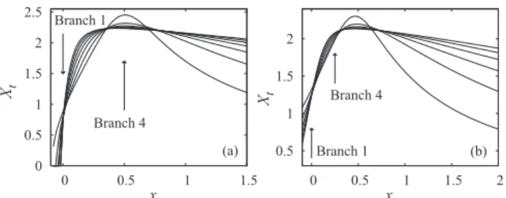
exists forn >1, as well as that predicted by the Coulomb gas theory in the rangen <1. This is illustrated in Fig.3, which shows the two leading temperaturelike scaled gaps for system sizesL=8, 10, 12, 14, and 16.
The data forXhin TableVagree well with the Coulomb
gas results, except near|n| =2. Poor finite-size convergence occurs nearn=2, and forn= −2, the whole eigenvalue spec-trum of finite systems collapses to |i| =2, corresponding
6 5 4 3 2
0 0.5 1 1.5 2
X
tn
FIG. 3. (Color online) The two leading thermal scaled gaps of the branch-1 model versus loop weightnfor even system sizesL=8 to 16. The scaled gaps are shown as thin lines, smoothly connecting a series of data points. The scaled gaps increase withLin most of the range ofn. Also shown are two thicker lines, of which one represents a constant scaling dimensionX=4 and the other the Coulomb gas result forXt. Extrapolation of the finite-size data indicates that the
leading gap (upper set of curves) converges toXt =4 forn <1 and
to the Coulomb gas result forXt forn >1. The second gap behaves
similarly but with the intervals ofninterchanged.
withXt =Xh=0. However, we expect a different result for
these scaling dimensions when the order of the limitsn→ −2 andL→ ∞is reversed.
The data for |n|10 show a divergent behavior of the scaled gaps, in agreement with the expected absence of criticality for large|n|. Extrapolations for|n|2 (not shown in TableV) are consistent with the presence of a marginally relevant operator at|n| =2. The ranges|n|>2 of branch 1 have earlier been identified [26] as lines of phase coexistence, separating two lattice-gas-like ordered phases. The associated vanishing scaling dimension corresponds with an eigenvector that is not invariant under lattice translations.
B. Branches 2 and 3
We followed a similar procedure in order to obtain the scaling dimensionsXtandXhas for branch 1. The extrapolated
results are shown in TableVI. The entries forXtatn=1 are
shown to indicate that the temperaturelike energy gaps of finite systems diverge for n→1. However, this is due to another eigenvalue of the transfer matrix that obscures the true scaling behavior for small system sizes. If one would first take the limit L→ ∞and then the limitn→1, a resultXt ≈2 is expected.
Forn=1, the finite-size results for the scaled magnetic gaps vanish, and the corresponding entryXh=0 is in line with the
entries for branch 2 withn >1.
TABLE VI. Numerical results for the temperature dimensionXt
and the magnetic dimensionXhof the branch-2 and branch-3 models.
Estimated numerical uncertainties in the last decimal place are given between parentheses.
n Xt (branch 2) Xh(branch 2) Xt (branch 3)
1.0 ∞ 0 (−) ∞
1.2 2.0 (?) 0.00 (2) 0.8 (1)
1.4 1.9 (1) 0.04 (2) 1.0 (2)
1.6 1.90 (5) 0.08 (1) 1.4 (?)
1.8 2.00 (5) 0.105 (5) 1.6 (2)
2.0 1.9 (1) 0.122 (2) 0 (−)
10 −0.2 (2) 0.0 (1) −0.1 (3)
20 0.0 (1) 0.0 (2) 0.0 (1)
30 0.00 (1) 0.000 (2) 0.00 (1)
A similar result is found for Xt on branch 3 at largen.
However, forn→2 the behavior is different and the thermal scaled gaps of finite systems vanish in this limit.
The finite-size data forXhon branch 2 withn <1.5 could
not be satisfactorily fitted with a power law. The assumption that Xh(L)Xh+a/lnL gave somewhat better behaved
results, but the errors are hard to estimate. In TableVI we base the error estimates on the differences between the above logarithmic fits and fits with a fixed power−1. Also forn=2 we used logarithmic fits, which yielded a best estimate not far from the exact valueXh=1/8. In the case of branch 3, the
free energies oscillate not only between even and odd systems, but also with a period four, and we did not produce meaningful estimates ofXh.
C. Branches 4 and 5
As noted in Sec.IV, the leading eigenvalues of the transfer matrices of finite branch-4 systems for n >−2 are equal to those for branch 5. Since this does not hold for the rest of the eigenvalue spectra, we perform separate analyses for the two branches. Unfortunately, the convergence of the scaled gaps is very poor, and we did not find accurate results. Power-law fits tend to yield finite-size exponents that vary considerably with system size, often assuming positive values. Logarithmic fitsXt(L)Xt+a/lnLwere not very
satisfactory either, because the finite-size data display an extremum as a function of the finite size for some values ofn. Under these circumstances, we take the branch-4 scaled gaps at system sizeL=16 as our final estimates. They are shown in TableVII. The difference with the result of the logarithmic fit, or 10 times the difference between theL=14 and 16 results, is quoted as a rough estimate of the error margin.
A similarly slow convergence is observed for the branch-5 scaled gaps. Forn <−2 we have the additional problem that the largest eigenvalues display a finite-size dependence not only with an odd-even alternation, but also with an effect of period 4. However, some observations can still be made. For large negativenthe scaled gaps tend to become very small, and forncloser to−2 they are at most a few tenths, and tend to decrease with increasingL. Forn= −2 the largest eigenvalues
TABLE VII. Fit results for the temperature dimension Xt and
the magnetic dimensionXh of the branch-4 and branch-5 models.
Estimated numerical uncertainties in the last decimal place are given between parentheses. The entries “0 (−)” indicate that the raw numerical data agree, up to numerical precision, with a vanishing result.
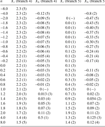
n Xt(branch 4) Xh(branch 4) Xt(branch 5) Xh(branch 5) −8.0 2.3 (5)
−4.0 2.3 (2) −0.12 (5) −0.8 (2)
−2.0 2.3 (2) −0.09 (5) 0 (−) −0.47 (5)
−1.8 2.3 (2) −0.08 (5) 0.0 (1) −0.43 (5)
−1.6 2.3 (2) −0.08 (5) 0.0 (1) −0.40 (5)
−1.4 2.3 (2) −0.08 (4) 0.0 (1) −0.37 (5)
−1.2 2.3 (2) −0.07 (5) 0.0 (1) −0.33 (5)
−1.0 2.3 (2) −0.07 (5) 0.0 (1) −0.30 (5)
−0.8 2.3 (2) −0.06 (5) 0.1 (1) −0.27 (5)
−0.6 2.2 (2) −0.06 (4) 0.1 (2) −0.24 (4)
−0.4 2.2 (1) −0.05 (4) 0.1 (2) −0.21 (4)
−0.2 2.2 (1) −0.05 (3) 0.1 (2) −0.17 (4) 0.0 2.2 (1) −0.04 (3) 0.1 (3)
0.2 2.2 (1) −0.03 (3) 0.2 (3) −0.11 (5) 0.4 2.2 (1) −0.03 (3) 0.3 (3) −0.08 (2) 0.6 2.2 (1) −0.02 (2) 0.3 (3) −0.05 (2) 0.8 2.2 (2) −0.01 (2) 0.4 (3) −0.02 (2)
1.0 2.1 (2) 0 (−) 0.5 (3) 0 (−)
1.2 2.0 (3) 0.013 (3) 0.7 (3) 0.02 (2) 1.4 2.0 (3) 0.03 (4) 0.9 (2) 0.054 (2)
1.6 1.9 (3) 0.05 (3) 1.1 (2) 0.07 (2)
1.8 1.8 (3) 0.07 (3) 1.5 (2) 0.09 (2)
2.0 1.7 (2) 0.11 (2) 1.9 (2) 0.11 (2)
4.0 1.4 (4) 0.5 (1) 1.3 (2) 0.125 (3)
8.0 1.5 (5) 1.4 (2) 0.12 (4)
become degenerate, which corresponds withXt =0. The final
estimates of Xt shown in Table VII for n >−2 are taken
from logarithmic fits, and the error estimates are taken as their differences with the scaled gaps atL=14. The entry at n=0 is obtained from interpolation between small negative and positive values of n, because the vertex weightc/n in Eq. (3) diverges atn=0. Similar numerical problems appear during analysis of the magnetic gaps as defined in Eq. (38). Thus, also the results for Xh in Table VII, and their error
estimates, are somewhat uncertain.
VI. LOCATION OF PHASE TRANSITIONS
In order to explore the physical properties of the seven branches of solvable models described in Table I, we per-formed some further numerical work. Without aiming at a complete coverage of the phase diagram, we wish to investigate the possible association of the solvable branches with lines of phase transitions or the location of these branches with respect to such phase transitions.
0 0.5 1 1.5 2 2.5 3
-2 -1.5 -1 -0.5 0 0.5
Xt
cn
Branch 1 Branch 2 Branch 3
(a)
0 0.02 0.04 0.06 0.08 0.1
-0.8 -0.4 0 0.4
Xh
cn Branch 1
Branch 2
(b)
FIG. 4. Scaled thermal (a) and magnetic (b) gaps versus cn
covering branches 1, 2, and 3 of the completely packed O(n) loop model withn=1.5. Results are shown for even system sizesL=4 to 20 for the thermal case, and forL=4 to 18 for the magnetic case. In panel (a) the scaled thermal gaps increase withL, on both the left and the right sides of the scale. Instead, in panel (b) the scaled magnetic gaps decrease on both sides. The data for Xt display cusps near
cn≈ −1.2, which are due to intersections between transfer-matrix
eigenvalues. Complex pairs of eigenvalues then appear in a range of cnfor system sizes equal to odd multiples of 2. The corresponding
data for these ranges are not shown in this figure. A. Branch 1
The completely packed nonintersecting O(n) loop model with |n|<2 on the square lattice belongs to the same universality classes as the dense phase of the O(n) model. For the latter model, the introduction of crossing bonds, as well as that of cubic vertices, leads to crossover to different universal behavior. Both of these perturbations are described by the cubic-crossover exponent given by Eq. (30), which is relevant in the dense O(n) phase. Thus, branch 1 is a locus of phase transitions in the (n,x,cn) parameter space, at least
for |n|<2. This was already illustrated for the dense O(n) phase by transfer-matrix calculations in Ref. [11]. For the present completely packed case, a few instances of the effect of a variation of the weights of the cubic and crossing-bond vertices on branch 1 will be included in the following sections treating branches 2–5.
B. Branches 2 and 3
For branches 2 and 3, onlyz-type andc-type vertices are present. These two branches exist only forn1. They merge at the end pointn=1, where the system reduces to a trivial case with effective weight 1 for each loop and each vertex. We first consider the thermal and magnetic scaled gapsXtandXh
of a system withn=1.5 as a function ofcn. Results are shown
in Figs.4. Several details can be noted. Atcn=0, which is the
location of branch 1, the scaled gaps are nicely approaching the values given by Eqs. (28). Furthermore, the curves forXt
show intersections close to the branch-1 point, with slopes that increase withL. Then a comparison with the scaling behavior expressed by Eq. (37), withytplaying the role of the exponent
of the cubic perturbationcn, shows that the cubic perturbation
is relevant on branch 1 atn=1.5, because the slopes increase withL. Slightly to the left of branch 2, intersections occur as well, but here the cubic weight seems to be irrelevant. Indeed, forcn<0 there exists a range about branch 2 where theXt
data are consistent with slow convergence to a value close to 2, independent ofcn. The data forcn<−1 appear to behave
irregularly due to finite-size effects with a period exceeding 0 1 2 3 4
-0.5 0 0.5 1
Xt
cn Branch 1, 2
(a)
0 0.05 0.1 0.15 0.2
-0.8 -0.4 0 0.4 0.8
Xh
cn Branch 1, 2
(b)
FIG. 5. Scaled thermal (a) and magnetic (b) gaps versus cn
covering branches 1 and 2 of the completely packed O(n) loop model withn=2. Results are shown for even system sizesL=4 to 18 for the thermal case and forL=4 to 16 for the magnetic case. In panel (a) the scaled thermal gaps increase withLnearcn=1, while the
scaled magnetic gaps instead decrease on the right-hand end of the scale.
2. However, the data withLrestricted to multiples of 4 allow convergence at the branch-3 point. The data withcn smaller
than the branch-3 value indicate that scaled gaps diverge with increasingL.
The results for Xh in Fig. 4(b) display a similar scaling
behavior near branches 1 and 2. At cn=0 (branch 1) the
data agree with convergence to the theoretical value given by Eq. (28). The slow apparent convergence forcn<0 indicates
the existence of a marginal or almost marginal temperature dimensionXt≈2. In the neighborhood of branch 3, theXh
data (not shown) lose transparency because of the irregular finite-size dependence. For cn significantly less than the
branch-3 value, as well as forcnsignificantly exceeding the
branch-2 value, the data are consistent with convergence to Xh=0, as expected for a phase dominated by cubic vertices.
Forn=2,cn>−2, again one finds divergent behavior of
the gapsXt, corresponding with a noncritical phase dominated
byc-type vertices. The same observation applies to the range where cn considerably exceeds the branch-1 value. Again,
complex eigenvalues occur near branch 3. The behavior ofXt
andXhin the neighborhood of branch 1, which coincides with
branch 2 forn=2, is shown in Figs.5. These data indicate that there exists a rangecn<0 where the cubic weight is marginal,
for whichXh=1/8 andXt =2.
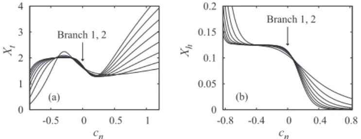
Next we consider the thermal and magnetic scaled gaps in the rangen >2. Figure6shows these quantities forn=10 as a function of the cubic weightcn=c/n, for a range of system
sizes, withzfixed atz=1. TheXtcurves are seen to display
minima, which become increasingly pronounced for larger system sizes, and whose location rapidly converges to the branch-2 valuecn=0.2. TheXhcurves instead monotonically
decrease as a function of cn, and they intersect at points
that rapidly approach the branch-2 value ofcn. Furthermore,
extrapolation of the two types of scaled gaps at the minima or at the intersections leads to values close to 0 (see also TableVI), strongly suggesting a first-order phase transition at branch 2. The scaled magnetic gaps forcn smaller than the
branch-2 value in this figure seem to diverge, as expected for a disordered phase. Instead, forcnexceeding the branch-2 value,
![TABLE IV. Fit results for the bulk free-energy density of branches 4 and 5, compared with the theoretical values f R given by Rietman [29].](https://thumb-us.123doks.com/thumbv2/123dok_us/8160217.2163542/10.911.80.834.194.597/table-results-density-branches-compared-theoretical-values-rietman.webp)