1659176.pdf

(1)

Research Article

Evaluating Operational Effects of Bus Lane with Intermittent

Priority under Connected Vehicle Environments

Dingxin Wu,

1,2,3

Wei Deng,

1

Yan Song,

3

Jian Wang,

4

and Dewen Kong

1 1_{School of Transportation, Southeast University, Si Pai Lou No. 2, Nanjing 210096, China}

2_{Key Laboratory for Traffic and Transportation Security of Jiangsu Province, Huaiyin Institute of Technology, Huaian 223003, China} 3_{Program on Chinese Cities, University of North Carolina at Chapel Hill, Chapel Hill, NC 27599, USA}

4_{School of Civil Engineering, Purdue University, West Lafayette, IN 47907, USA} Correspondence should be addressed to Dingxin Wu; [email protected]

Received 31 August 2016; Revised 26 January 2017; Accepted 6 March 2017; Published 19 April 2017

Academic Editor: Aura Reggiani

Copyright © 2017 Dingxin Wu et al. This is an open access article distributed under the Creative Commons Attribution License, which permits unrestricted use, distribution, and reproduction in any medium, provided the original work is properly cited.

Bus lane with intermittent priority (BLIP) is an innovative method to improve the reliability of bus services while promoting efficient usage of road resources. Vehicle-to-vehicle (V2V) communication is an advanced technology that can greatly enhance the vehicle mobility, improve traffic safety, and alleviate traffic jams. To explore the benefits of BLIP operation under a connected environment, this study proposed a three-lane cellular automata (CA) model under opening boundary condition. In particular, a mandatory BLIP lane-changing rule is developed to analyze special asymmetric lane-changing behaviors. To improve the simulation accuracy, a smaller cell size is used in the CA model. Through massive numerical simulations, the benefits and influences of BLIP are explored in this paper. They include impacts on neighborhood lanes such as traffic density increasing and average speed decreasing, lane-changing behaviors, lane usage, and the impacts of bus departure interval and clear distance on the road capacity of BLIP. Analysis of traffic flow characteristics of BLIP reveals that there is a strong relationship among bus departure interval, clear distance, and road capacity. Furthermore, setting conditions for deployment of BLIP under the V2V environment such as reasonable departure interval, clear distance, and traffic density are obtained.

1. Introduction

To reduce traffic congestion in urban areas, many strategies have been proposed to improve the operational efficiency and attractiveness of public transportation systems. The dedicated bus lane (DBL) is perhaps one of the most popular bus priority strategies that seeks to provide high-quality transit service and improve operation speed. While DBL is able to improve the service level of the transit system, it requires the reservation of a whole lane for buses and forbids the entrance of private vehicles during a certain period. This may reduce the usage of limited road resources, leading to serious congestion of neighborhood lanes. To address this problem, Eichler [1] proposed an innovative bus priority approach called the bus lane with intermittent priority (BLIP). The basic idea of the original BLIP concept is to divide the road segment into a few sequential sections. The length of each section is predetermined by the geometry of road networks,

like intersections, which means each section may not be equal in length. The section-based BLIP works as follows: when a bus is approaching a roadway section, the BLIP in this roadway section becomes a bus lane; private vehicles running in front of the bus are required to leave the BLIP lane for the oncoming bus using variable message signs; when the bus passes this roadways section, the BLIP lane is reopened to private traffic again; private vehicles behind the bus are allowed to enter the BLIP lane at any time [2, 3].

Numerous researches have been conducted to explore the system components. Implementation of BLIP relies on a number of transportation infrastructures such as automatic vehicle location, central control system, information panel, in-pavement lights, and bus detection [4, 5]. A simulation conducted by US Department of Transportation reveals that the BLIP reduces the travel time by 14% through improv-ing the intersection delays [6]. This outcome, however, is challenged by some other studies where BLIP is found to

(2)

negatively contribute to traffic delay and the road capacity [1, 2]. Albeit so many efforts devoted to the study of BLIP, a number of associated challenges still prevent the fully exploit of its potentials. First, the road capacity is still wasted too much if BLIP is too long; second, the sections of varied lengths may cause unsymmetric benefits of BLIP. To address this problem, Wu et al. [7] proposed a connected vehicles (CV) based BLIP, where the section lengths are assumed to be fixed and all vehicles are capable of vehicle-to-vehicle (V2V) communications to assist lane-changing decisions. Based on V2V communication, real-time information such as vehicular location and speed could be exchanged between vehicles. A predetermined clear distance for private vehicles could then be set in BLIP to clear the road for coming buses. Although the impact of BLIP is investigated in recent researches, studies related to BLIP under V2V environment are very rare and some major issues still remain untacked, for example, the interrelationship between fundamental dia-gram, speed-density relationship, and road capacity of V2V-based BLIP, the impact of various factors on BLIP such as lane-changing rules, long bus departure intervals, vehicle lengths, and acceleration, and frequently ping-pong lane-changing pattern. This prevents the full exploration of the inhomogeneous phenomena associated with the bus priority strategy. Furthermore, as one of the most promising enabler technologies, a comprehensive guideline for implementation of BLIP in the connected environment and an approach to quantify the corresponding impact on traffic flow and road capacity are yet to be found.

Most of existing studies explore BLIP using theoretical methods such as kinematic wave theory. However, these studies mainly focus on analyzing the macroscopic traffic flow characteristics and pay little attention to microscopic details which are fundamental for operation of BLIP. In addition, theoretical methods are not flexible enough to deal with complex traffic environments like V2V communication [8]. In certain context, the simulation-based method is more robust which allows researchers to comprehensively study the traffic flow through holistically considering the potential impact factors. For example, the cellular automaton (CA) had been proved to be a powerful tool to study traffic flow under both macro- and microenvironments [9]. It is, thereby, extensively adopted to study the traffic flow pattern.

The CA model (NS) for a single lane was first formulated by Kai and Schreckenberg [10]. Based on the NS model, CA models have been extended to study two-lane and three-lane traffic flow models. Chowdhury et al. [11] extended it to a two-lane model with stochastic two-lane change rule. Daoudia and Moussa [12] used it to build a three-lane model with sym-metric lane change rule. Several attempts have been made so far in this direction, and different lane-changing procedures have been proposed [13–16]. CA models for mixed vehicle traffic such as mixed private vehicles with buses or trucks have also been studied [15, 17–19]. These studies found that the CA model can efficiently characterize some traffic flow phenomenon occuring in multilane and mixed traffic flow scenarios. To take advantage of CA model, this study pro-posed a three-lane CA model to study the influence of V2V-based BLIP on urban traffic flow.

The paper is structured as follows: the next section presents the modeling framework and lane-changing rules for BLIP in the V2V communication environment. The per-formance of BLIP including road capacity, lane usage under various lane-changing behaviors, bus departure intervals, and clear distances is explored in Section 3. The final section concludes this research and proposes further research topics.

2. Model

In this section, a three-lane CA model for BLIP under V2V environment is presented. The traffic condition under which the BLIP can be implemented will also be studied.

2.1. Model Definition. The hypothetical BLIP simulation

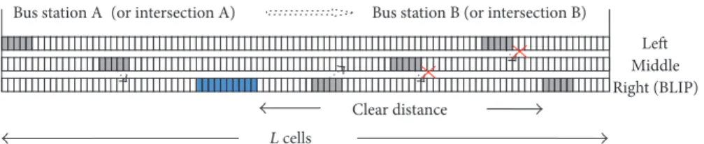
sys-tem consists of three parallel single lanes (left, middle, and right). It is based on V2V technology, which means each private vehicle can evaluate whether it is in the clear distance range of a rear bus or not according to real-time information (like location and speed). Since bus stops are often deployed near intersections to utilize the red-light time for boarding passengers [20, 21], thus, the BLIP lane itself can be seen as the key factor in urban traffic flow and the model focuses on how the BLIP affects traffic flow on the road and does not take bus stations and intersections into account.

The model is defined on a one-dimensional array of 𝐿 cells per lane. In previous CA models, each cell has a uniform length of 7.5 m, and each vehicle has the uniform size and occupies exactly one cell. Such cell size is too coarse, which leads to unrealistic acceleration rates. A smaller cell size can simulate the acceleration behavior with higher resolution which can mimic the physical features of vehicular move-ments better [22, 23]. In this study, each cell represents a divi-sion of the road of 1.5 m. There are two types of vehicles on the road: regular cars with maximum speed V𝑐max = 15 cells/s (≈81 km/h) and buses with maximum speedV𝑏max= 10 cells/s (≈54 km/h). Each car occupies 5 cells and each bus occupies 10 cells. Clear distance for bus𝑙cd ∈ {150m, 300m, 450m,

600m}. One time step corresponds to one second in practice. Most key variables and parameters used in the model are summarized in Variables and Parameters.

2.2. Rules for Vehicle Movements. As can be seen from

Figure 1, with each time step, if the firstV𝑐_maxcells of each lane are empty and a vehicle is allowed to enter the left boundary of the road (𝑝 ≤ 𝑝in), a new vehicle would be created at the left boundary of each lane and runs forward at maximum speed. When a vehicle reaches the end of the lane, it is removed from the right boundary if the vehicle is allowed to leave (𝑝 ≤ 𝑝out). Otherwise, it remains in its position. Particularly, with every time interval𝑡depart, a new bus𝑖is created at the left of the BLIP lane, which means that bus𝑖departs from bus station A (or intersection A). When the bus𝑖reaches the right boundary of the lane, it is removed from the system (if

𝑝 ≤ 𝑝out), which means that the bus reaches bus station B (or intersection B). Each bus can only operate in the BLIP (right) lane and is not allowed to change its lane at any time.

(3)

Middle Right (BLIP)

Left

L cells

Clear distance

Bus station B (or intersection B) Bus station A (or intersection A)

Figure 1: Diagram of three-lane traffic using V2V-based BLIP.

represents the position of the vehicle𝑖in lane𝑗, then gap𝑗_𝑖 =

𝑥𝑗_𝑖+1 − 𝑥𝑗_𝑖 − 𝑙𝑗_𝑖+1. This variable determines the progress of all vehicles. The randomization parameter𝑝rand= 0.25 is used. At each discrete time step, the following four rules are used to update the movements of all vehicles.

(1) Acceleration.If the velocity of a car (or a bus)𝑖in lane𝑗is

lower thanV𝑐max(orV𝑏max) and if there is enough space ahead (V𝑗_𝑖 ≤gap𝑗_𝑖 − 1), then the speed is increased by one; that is,

if (V𝑗_𝑖 ≤gap𝑗_𝑖 − 1)thenV𝑗_𝑖 =min(V𝑐max,V𝑗𝑖 + 1) 𝑜𝑟V𝑗𝑖 = min(V𝑏max,V𝑗𝑖+ 1).

(2) Deceleration.If the next vehicle ahead is too close (V_𝑖𝑗 ≥

gap𝑗_𝑖 + 1), then speed is reduced to gap𝑗_𝑖; that is,

ifV𝑗_𝑖 ≥gap𝑗_𝑖+ 1thenV𝑗_𝑖 =gap𝑗_𝑖.

(3) Randomization. The velocity of each vehicle (if greater

than zero) is decreased by one with probability𝑝rand; that is,

with𝑝rand:V𝑗_𝑖 =max(V𝑗_𝑖 − 1, 0).

(4) Position Update.Each vehicle movesV𝑗_𝑖 cells forward at

each time step.

2.3. Lane-Changing Rules. If the BLIP system has been

equipped with V2V technology, drivers can easily get real-time-space headways in different lanes and decide whether to change lanes or not. Generally, lane-changing rules can be symmetric or asymmetric with respect to the lanes or to the vehicles. All changing behaviors in this model are divided into the following two categories: the common lane-changing with the symmetric rule, where the regular cars change lanes randomly to a neighborhood lane if necessary; and BLIP lane-changing with the asymmetric rule, which means some cars are forced to leave the BLIP lane due to an oncoming bus if they are in the range of the rear bus’s clear distance.

2.3.1. Common Lane-Changing. In normal driving contexts,

the driver needs to change lanes to seek a better driving environment; this is labeled as common lane-changing in this study. To mimic the common lane-changing behavior, the following three essential criteria are used in the proposed model:(1)the incentive criterion: a faster car wants to keep a desired high speed or avoid jamming traffic;(2)the security criterion: a driver only change lanes when it is safe and his/her behavior does not affect the movements of other vehicles on target lane; and(3)the time criterion: a car must remain in the

original lane for at least 4 seconds before it starts to change lanes to avoid ping-pong lane-changing behaviors [14]. The methods to model these criteria of common lane-changing behaviors are presented as follows.

Let gap-f ront𝑘_𝑖 (resp., gap-rear𝑘_𝑖) be the number of free cells between a car 𝑖 in lane 𝑗 and its front (resp., rear) neighboring car in target lane𝑘. When the car𝑖is blocked by the nearest vehicle ahead and cannot obtain its desired speed at time𝑡, it might try to find a safe gap in the adjacent lane and change lanes. If gap-f ront𝑘_𝑖 in target lane𝑘is greater than gap𝑗_𝑖 in its original lane𝑗, the car𝑖could have a motivation to change lanes. If all lane-changing criteria are satisfied, it can make a discretionary lane change to any feasible lane. As shown in Figure 1, for a car in the left or the right lane, it can only change to the middle lane. For a car in the middle lane which is not in a rear bus’s clear distance, it will change to an available adjacent lane, either to the left lane or to the right lane. If both adjacent lanes (left and right) are available, a driver is encouraged to change to the left for two major reasons:(1)a better use of the middle lane for those cars in the BLIP lane that are forced to move in; and(2)encouraging a faster car to move to the left. Common lane-changing rules can be summarized as follows:

Ifgap𝑗_𝑖 <min(V𝑐_max,V𝑗_𝑖+ 1)

&gap-f ront𝑘_𝑖 ≥min(V𝑐_max,V𝑗_𝑖 + 1)

&gap-rear𝑘_𝑖 ≥min(V𝑐_max,V𝑗_𝑖+1)−min(V𝑐_max,V𝑘_𝑖+1+1)+

gap_safety

thencar𝑖changes lane from𝑗to𝑘.

2.3.2. BLIP Lane-Changing. As can be seen in Figure 1, cars in

the left (or middle) lane and within the clear distance range of a rear bus are not encouraged to change lanes to the middle (or right) lane. This provides more spaces for mandatory lane-changing from the BLIP lane to the middle lane. Cars in the right lane and just in the clear distance range of a rear bus are forced to leave the BLIP lane as soon as possible if all lane-changing criterions are satisfied. If there is no safe gap, they will remain in the BLIP lane and try to merge to the middle lane again at next time step, which can be described as follows:

Ifgap-f ront𝑘_𝑖 ≥gap_safety

&gap-rear𝑘_𝑖 ≥min(V𝑐max,V

𝑗

𝑖+1)−min(V𝑐max,V𝑘𝑖+1+1)+

gapsafety

(4)

Those cars in the BLIP lane but not in the clear distance for a bus are not required to leave the lane for the oncoming buses.

3. Simulations and Discussions

In this section, we conduct numerical simulations of an urban roadway under the opening boundary condition using the three-lane CA model. The main road length is 1600 cells (2400 meters). The first 10000 time steps are discarded to reduce the negative effect of the transient time. The results are obtained from 10001 to 10600 time steps. We discuss all sim-ulations under the following two traffic situations: the three-lane urban road with no bus priority and no BLIP three- lane-chang-ing (labeled as Case A) and the three-lane urban road with the BLIP strategy (labeled as Case B).

Denote𝑁_𝑗,type(𝑡)as the number of vehicles in lane𝑗at time𝑡(pcu/lane, passenger car unit/lane), type ∈ {car,bus}. Let𝜌_𝑗(𝑡)denote the traffic density of lane𝑗at time𝑡(pcu/km), andV_𝑗(𝑡) (km/h), and𝑗 ∈ {left,middle,right} denotes the average velocity of lane𝑗. The following equations are used to calculate𝜌_𝑗(𝑡)andV_𝑗(𝑡), respectively:

𝜌_𝑗(𝑡) = 5 × 𝑁𝑗,car(𝑡)

𝐿 +

10 × 𝑁_𝑗,bus(𝑡)

𝐿 ,

V_𝑗(𝑡) = { 1

[𝑁_𝑗,car(𝑡) + 𝑁𝑗,bus(𝑡)]

}

× [ [

𝑁𝑗,car(𝑡)

∑

𝑖=1 V

𝑗

𝑖 +

𝑁𝑗,bus(𝑡)

∑

𝑖=1 V

𝑗

𝑖]

] .

(1)

In this simulation, a vehicle is inserted into the left boundary of each lane with the entry probability𝑝in(0.025 ≤

𝑝in≤ 1). It determines the input of traffic flow.

To analyze the function of BLIP, eight aspects are explored: effects of BLIP, average traveling time, effects of bus departure interval, effects of clear distance, lane change behavior, lane usage, traffic capacity, and suitable traffic conditions.

3.1. Effects of BLIP. Simulation is conducted with different

lane-changing rules to evaluate the performance of the BLIP strategy, including time-space distribution of traffic flow, average speed, average delay, lane-changing rate and frequen-cy, lane usage, average bus traveling time saving, and road capacity loss.

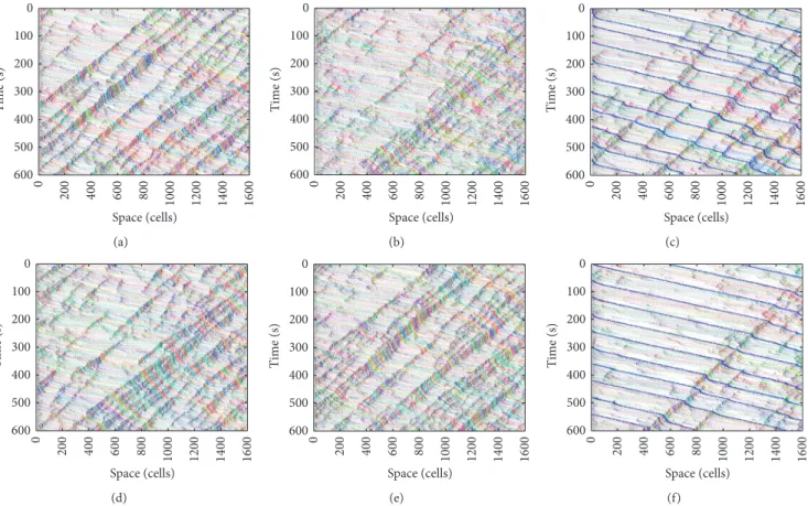
3.1.1. Traffic Time-Space Distributions. Figure 2 shows the

time-space distributions of traffic flow of the right lane under both Case A and Case B. The initial inputs for the variables are set as follows:𝑡depart= 60 s,𝑙cd= 300 m,𝑝rand= 0.25,𝑝in= 1, and𝑝out= 0.7. The blue lines in Figures 2(c) and 2(f) represent trajectory of buses.

As we can see from Figure 2(c), upstream cars will always slow down to follow buses or try to change lanes to overtake the buses in Case A. Additionally, some buses cannot main-tain their speeds due to downstream congestion and this leads

to a decline in service quality. Such a situation is significantly improved by introducing the BLIP strategy (Figure 2(f)). The downstream cars in the BLIP lane will be forced to change lanes (mandatory lane-changing) when a bus is coming. The trajectory of buses is consistent with the bus departure interval and is less influenced by general traffic in Case B. Recall that the mandatory lane changes are performed only when those cars are in a clear distance range of a rear bus, which makes merging behaviors more complex in the middle and right lane. Besides, mandatory BLIP lane-changing may induce traffic jams in the middle lane (Figure 2(e)). Due to the BLIP, the traffic density of the right lane in front of buses decreases. This makes the buses move more smoothly with higher speeds and fewer delays.

3.1.2. Average Speed Distributions. Average speeds of different

lanes are also studied and the inputs of variables are the same as those in Section 3.1.1. Figure 3 presents the average speed of each lane in Case A and Case B. It shows that the average speed difference between the different lanes is very small under the common lane-changing rule in Case A. But for the BLIP lane-changing rule, the average speed of the BLIP lane increases by 50% as compared with its previous speed. Each peak of average speed in the BLIP lane corresponds to a trough in the left and middle lane when there are buses pass-ing through the BLIP lane. Simulation results show that buses can maintain a higher speed even in higher traffic density due to the BLIP strategy. The average speeds of vehicles in both left and middle lanes in Case B also increase due to the open boundary and BLIP strategy.

Figure 4(a) presents the average bus speed in Case A and Case B. It is obvious that the average speed of buses in Case B is much higher than in Case A. The mean of average bus speed in Case A is about 35 km/h and increases to over 50 km/h in Case B. This is perhaps because the disruptive behavior of reg-ular cars on buses is significantly reduced by introducing the BLIP strategy. Figure 4(b) compares the difference between each average bus speed and the mean of average bus speed in each time slot. It reveals that average bus speed in Case A deviates from the mean more seriously than in Case B.

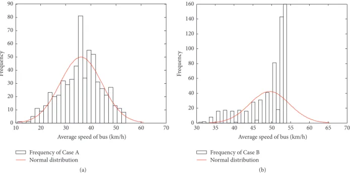
Histograms shown in Figure 5 further justify such phe-nomenon. Figure 5(a) obeys normal distribution, and it also illustrates that 36 km/h is the mean of average bus speed in Case A. However, atypical and asymmetric bus speed distribution in Case B with dispersion and higher speed easily ensures that buses have a smooth ride and are fuel efficient which improves bus service significantly (Figure 5(b)).

3.2. Average Traveling Time. The main purpose of providing

(5)

0 100 200 300 400 500 600 T ime (s) Space (cells)

1200 1400 1600

1000 800 60 0 40 0 200 0 (a) 0 100 200 300 400 500 600 Ti m e ( s) Space (cells)

1200 1400 1600

1000 800 60 0 40 0 200 0 (b) 0 100 200 300 400 500 600 Ti m e ( s) Space (cells)

1200 1400 1600

1000 800 60 0 40 0 200 0 (c) 0 100 200 300 400 500 600 Ti m e ( s) Space (cells)

1200 1400 1600

1000 800 60 0 40 0 200 0 (d) 0 100 200 300 400 500 600 Ti m e ( s) Space (cells)

1200 1400 1600

1000 800 60 0 40 0 200 0 (e) 0 100 200 300 400 500 600 Ti m e ( s) Space (cells)

1200 1400 1600

1000 800 60 0 40 0 200 0 (f)

Figure 2: space distributions of Case A (a, b, c) and Case B (d, e, f). (a) space distribution of the left lane in Case A. (b) Time-space distribution of the middle lane in Case A. (c) Time-Time-space distribution of the right lane in Case A. (d) Time-Time-space distribution of the left lane in Case B. (e) Time-space distribution of the middle lane in Case B. (f) Time-space distribution of the right lane in Case B.

15 20 25 30 35 40 45 50 55 60 65

Case A, left lane Case A, blip lane

Case B, left lane Case B, blip lane

100 200 300 400 500 600 0 A verag e sp eed (v eh/km) Time (s) (a)

Case A, middle lane Case A, blip lane

Case B, middle lane Case B, blip lane

100 200 300 400 500 600 0 15 20 25 30 35 40 45 50 55 60 65 Time (s) A verag e sp eed (v eh/km) (b)

(6)

10 15 20 25 30 35 40 45 50 55

Case A: average speed of bus Case B: average speed of bus

100 200 300 400 500 600 0

A

verag

e sp

eed (km/h)

Time (s)

(a)

Case A: average speed of bus Case B: average speed of bus

100 200 300 400 500 600 700 0

Time (s)

−30

−25

−20

−15

−10

−5 0 5 10 15 20

D

evia

tio

n

s f

ro

m t

h

e me

an

(b)

Figure 4: Average speed distributions of Case A and Case B. (a) Average bus speed in Case A and Case B. (b) Deviations from the mean of average bus speed in Case A and Case B.

Frequency of Case A Normal distribution 0

10 20 30 40 50 60 70 80 90

F

req

uenc

y

20 30 40 50 60 70 10

Average speed of bus (km/h)

(a)

Frequency of Case B Normal distribution

35 40 45 50 55 60 65 70 30

0 20 40 60 80 100 120 140 160

F

req

uenc

y

Average speed of bus (km/h)

(b)

Figure 5: Histograms of average bus speed in Case A and Case B. (a) Histograms of average bus speed in Case A. (b) Histograms of average bus speed in Case B.

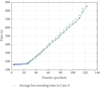
Figure 7 indicates that, by introducing temporary prior-ity, the travel time is reduced by 5% when the traffic density is within the range of[40, 80]pcu/km. The reduction reaches up to 7% when traffic density is around 45 pcu/km, which reduces bus traveling time delay and passenger waiting time and improves service reliability.

3.3. Effects of Bus Departure Interval. Figure 8 shows the

speed-density relationship of the BLIP lane in Case B at different bus departure intervals. The initial inputs for each

(7)

Average bus traveling time in Case A Average bus traveling time in Case B

20 40 60 80 100 120 140 0

100 200 300 400 500 600 700 800 900

Density (pcu/km)

T

ime (s)

Figure 6: Average bus traveling time in Case A and Case B in different traffic density scenarios.

BLIP. Longer bus departure interval is recommended because it improves average speed, traffic density, and road capacity of the right lane.

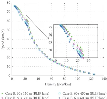
3.4. Effects of Clear Distance. Figure 9 illustrates the

speed-density relationship of the BLIP lane in Case A and Case B with different clear distances. The simulation scenario is based on the following variables:𝑙cd∈ {150m, 300m, 450m,

600m}, 𝑡depart = 60 s,𝑝rand = 0.25, 𝑝in = 1, and𝑝out = 0.7. As shown here, clear distance has a certain impact on the speed and traffic density. While a larger clear distance can provide more space for buses, it also leads to more lane-changing behaviors and brings confusion to traffic flow. Therefore, more cars are forced to the middle lane with clear distance increasing when traffic density is within the range of[0, 40]pcu/km, because there is enough space for those cars to change their lane from the right to middle. And there will be more cars going back to the right lane after a bus passes within the traffic density area. It leads to more lane-changing behaviors and causes lower average speed of BLIP lane. Similarly, clear distance changing may also cause the change of the traffic density. Smaller clear distance offers higher density and helps to improve road capacity.

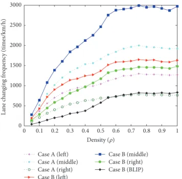
3.5. Lane Change Behavior. Frequent and large numbers of

lane changes not only negatively affect the traffic flows but also reduce the comfortability of driving. Here, we define LCf requency(𝑗)(times/lane/hour) and LCrate(𝑗) (lane-changing rate) as functions of average traffic density.𝑁_𝑖𝑗is the number of lane changes for vehicle𝑖in lane𝑗, per kilometer(Δ𝑥)of road, and for each time interval(Δ𝑡)[24].𝑁is the total num-ber of vehicles in lane𝑗for each time interval(Δ𝑡). The fol-lowing variables,𝑙cd= 150 m,𝑡depart= 60 s,𝑝rand= 0.25,𝑝in= 1,

and𝑝out= 0.7, are used in this simulation scenario to evaluate both symmetric and asymmetric lane change behaviors.

LCf requency(𝑗)= 𝑛

∑

𝑖=1

𝑁_𝑖𝑗 Δ𝑥 × Δ𝑡,

LCrate(𝑗)=

𝑁_𝑖𝑗 𝑁.

(2)

(8)

Reducing of bus operation time

20 40 60 80 100 120 140 0

Density (pcu/km) 0

10 20 30 40 50 60 70 80

Ti

m

e (

s)

(a)

Proportion of reducing time 0

1 2 3 4 5 6 7

Prop

or

ti

on

(

%

)

20 40 60 80 100 120 140 0

Density (pcu/km)

(b)

Figure 7: Average bus traveling time saving by BLIP in different traffic density scenarios. (a) Average bus traveling time saving by BLIP. (b) Proportion of average bus traveling time saving by BLIP.

20 40 60 80 100 120 140 0

0 10 20 30 40 50 60 70 80

Sp

eed (km/h)

10 20 30 40 0

60 65 70 75

Density (pcu/km) Case B,60s300m (BLIP lane)

Case B,150s300m (BLIP lane) Case B,90s300m (BLIP lane)

Case B,120s300m (BLIP lane)

Figure 8: Speed-density relationship under various bus departure interval factors.

3.6. Lane Usage. Here, we define 𝐿usage(𝑗) (total length of

vehicles/length of lane) as functions of average traffic density.

𝑙𝑗_𝑖 is the length of car𝑖in lane𝑗.𝐿is the length of lane𝑗.

𝐿usage(𝑗)=

∑𝑛_𝑖=1𝑙_𝑖𝑗

𝐿 . (3)

We present Figure 12 in order to clarify how the lane usage changes each lane between Case A and Case B. When the traffic density increases, the road occupancy rate grows sig-nificantly, whereas, for𝜌 ∈ [0.1, 0.4]in Case A, there are only

0 10 20 30 40 50 60 70 80

Sp

eed (km/h)

10 20 30 0

60 65 70 75

Case B,60s150m (BLIP lane) Case B,60s300m (BLIP lane)

Case B,60s450m (BLIP lane) Case B,60s600m (BLIP lane) Density (pcu/km)

140 120 100 80 60 40 20 0

Figure 9: Speed-density relationship under various clear distance factors.

(9)

Case A (left) Case A (middle) Case A (right) Case B (left)

Case B (middle) Case B (right) Case B (BLIP) 0

500 1000 1500 2000 2500 3000

L

ane c

h

an

gin

g f

req

uenc

y (times/km/h)

0.1 0.2 0.3 0.4 0.5 0.6 0.7 0.8 0.9 1 0

Density (𝜌)

Figure 10: Lane-changing frequency of each lane with traffic density increasing in Case A and Case B.

2 4 6 8 10 12 14 16 18 20 22

L

ane c

h

an

gin

g ra

te (%)

0.1 0.2 0.3 0.4 0.5 0.6 0.7 0.8 0.9 1 0

Density (𝜌) Case A (left)

Case A (middle) Case A (right) Case B (left)

Case B (middle) Case B (right) Case B (BLIP)

Figure 11: Lane-changing rate of each lane with traffic density increasing in Case A and Case B.

that of the middle lane and both are up to 10% higher than that in the right. Simulation results clearly indicate that cars are now predominantly in the left and the middle lane rather than in the right lane when buses are passing by.

3.7. Traffic Capacity. Buses are generally seen as disturbances

and slow-moving bottlenecks in traffic flow. Due to the BLIP strategy, it is hard to calculate traffic capacity by measuring

Case A (left) Case A (middle)

Case A (right) Case B (right)

0.1 0.2 0.3 0.4 0.5 0.6 0.7 0.8 0.9 1 0

Density (𝜌) 0

10 20 30 40 50 60

Road o

cc

u

pa

nc

y ra

te

(%)

Case B (left) Case B (middle)

Figure 12: Lane usage of Case A and Case B.

the saturation flow of the right lane because the traffic flow is dynamically disturbed by the moving buses. But it is not difficult to determine the traffic capacity of each lane using CA simulation.

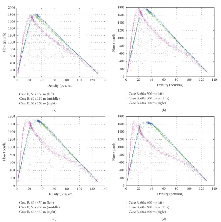
Figure 13 presents the density-flow relationships with different clear distance in Case B. It is observed that traffic flow of each lane decreases from more than 1800 pcu/h to about 1700 pcu/h with clear distance increasing, and that causes more road capacity loss. And the maximum traffic flow occurs at a lower traffic density (𝜌 < 40pcu/km) than that in the case with smaller clear distance. For the density-flow curve of the right lane, its right part is almost like an inclined straight line, which becomes more and more bent with clear distance rises.

The fundamental diagrams of the individual lanes also show that the maximum traffic flow of the middle lane is greater than the maximum traffic flow of the left and right lane. It illustrates that the middle lane has the larger saturation flow and higher traffic density than the other two lanes. Because a moving road section of the right lane would be prohibited for some cars, the traffic breaks down first in the right lane, while it still stays stable in the left or middle lane. Traffic flow drops rapidly relative to the other two lanes when𝜌 ≈ 20pcu/km. The values where the maximum flow is reached depend on different combinations of bus departure interval and clear distance.

(10)

20 40 60 80 100 120 140 0

0 200 400 600 800 1000 1200 1400 1600 1800 2000

Flo

w (p

cu/h)

Case B, 60 s 150 m (right) Case B, 60 s 150 m (middle) Case B, 60 s 150 m (left)

Density (pcu/km)

(a)

20 40 60 80 100 120 140 0

0 200 400 600 800 1000 1200 1400 1600 1800

Flo

w (p

cu/h)

Density (pcu/km)

(b)

0 200 400 600 800 1000 1200 1400 1600 1800

Flo

w (p

cu/h)

20 40 60 80 100 120 140 0

Density (pcu/km)

(c)

20 40 60 80 100 120 140 0

0 200 400 600 800 1000 1200 1400 1600 1800

Flo

w (p

cu/h)

Density (pcu/km)

(d)

Figure 13: Density-flow relationships with different clear distance in Case B. (a)𝑙_cd= 150 m. (b)𝑙_cd= 300 m. (c)𝑙_cd= 450 m. (d)𝑙_cd= 600 m.

capacity is reached at a smaller clear distance and a larger bus departure interval.

The maximum road capacity is obtained when𝑙cd= 150 m and 𝑡depart = 120 s and is slightly greater than 5500 pcu/h. The minimum of total capacity loss is less than 100 pcu/h for three lanes. And the minimum capacity is achieved when

𝑙cd= 600 m and𝑡depart= 60 s, which is slightly smaller than 5100 pcu/h.

3.8. Suitable Traffic Conditions. Simulation results in the

above sections show that the operational effects of the BLIP strategy are highly affected by traffic parameters in the three-lane road segment. Based on the results, the recommenda-tions of traffic condirecommenda-tions that are most suitable for BLIP

(11)

Case A: road capacity of three lanes (pcu/h) Case B: road capacity of three lanes when clear Case B: road capacity of three lanes when clear Case B: road capacity of three lanes when clear Case B: road capacity of three lanes when clear Case B: average density for max traffic flow Case B: average density for max traffic flow Case B: average density for max traffic flow Case B: average density for max traffic flow

60 90 120 150

distance = 150m (pcu/h)

when cleardistance = 150m (pcu/km) when cleardistance = 300m (pcu/km) when cleardistance = 450m (pcu/km) when cleardistance = 600m (pcu/km) 4800

4900 5000 5100 5200 5300 5400 5500 5600 5700

0 5 10 15 20 25 30 35

(s)

(a)

4800 4900 5000 5100 5200 5300 5400 5500 5600

150 300 450 600 0

5 10 15 20 25 30 35

Case B: road capacity of three lanes when Case B: road capacity of three lanes when Case B: road capacity of three lanes when Case B: road capacity of three lanes when Case B: average density for max traffic flow Case B: average density for max traffic flow Case B: average density for max traffic flow Case B: average density for max traffic flow departure interva_{l = 60}s (pcu/h) departure_{interval = 90}s (pcu/h) departureinterval = 120s (pcu/h) departureinterval = 150s (pcu/h) when departureinterval = 60s (pcu/km) when departure interva_{l = 90}s (pcu/km) when departure_{interval = 120}s (pcu/km) when departure interval = 150s (pcu/km)

(m)

(b)

Figure 14: Road capacity of three lanes in Case A and Case B with different bus departure interval and clear distance combinations. (a) Road capacity of three lanes with different bus departure intervals. (b) Road capacity of three lanes with different distances.

Table 1: Suitable traffic conditions for BLIP implementation.

Bus departure interval Clear distance Traffic density

Lower limit 90 s 150 m 30 pcu/km

Upper limit — 300 m 90 pcu/km

very high traffic density, in which general traffic could barely change lanes to provide temporary priority for buses. The above information is critical to the BLIP operation practices, which guarantee that the V2V-based BLIP plays a positive role in promoting bus service quality.

4. Conclusion

This paper focuses on building a simulation framework to evaluate a V2V based BLIP system. Microscopic traffic characteristics such as lane-changing behaviors and lane usage are investigated by setting a new BLIP lane-changing rule. The three-lane CA model provides a useful tool to study the influence of the BLIP on urban roads, explore suitable traffic conditions, and make better decisions in an application of the BLIP strategy under a connected vehicle environment. It is found that there are higher average speed and lower traffic density in the BLIP lane with respect to the ordinary

lane. And it is also found that larger clear distance and higher bus departure frequency both increase the impact on general traffic under the BLIP strategy. There is no doubt that the BLIP strategy could promote bus speed and save bus traveling time at a certain traffic condition range, but at the same time it unavoidably reduces road capacity. The BLIP strategy par-tially sacrifices the interests of car users to support bus riders, which seems reasonable for transportation equality. Accord-ing to simulation results, the BLIP strategy reduces the total capacity of three lanes by nearly 500 pcu/h in the worst situa-tion. The BLIP strategy has a positive effect only when the traffic condition is within the range of𝜌 ∈ [30, 90]pcu/km,

𝑙cd∈ [150, 300]m, and𝑡depart∈ [90, +∞)s.

(12)

using our method if the model is slightly improved. Our work concentrates on studying the BLIP strategy on a three-lane roadway. Since our model proves that BLIP strategy works well in various scenarios, the benefits of the BLIP strategy would be more remarkable when there are four or more lanes in the roadway. More extensive simulation numerical experi-ments need to be conducted to assess the effectiveness of the proposed strategy under different patterns of bus stops, pas-senger volumes, and a probability of private drivers who obey mandatory lane-changing rules.

Variables and Parameters

Variables

𝑥𝑗_𝑖: Position of vehicle𝑖in lane𝑗 V𝑗_𝑖: Speed of vehicle𝑖in lane𝑗

gap𝑗_𝑖: Free sites ahead of vehicle𝑖in original lane𝑗 gap-f ront𝑘_𝑖: Free sites ahead of vehicle𝑖in target lane𝑘 gap-rear𝑘_𝑖: Free sites rear of vehicle𝑖in target lane𝑘 gapsafety: Safety gap for each vehicle

𝑙cd: Length of clear distance

𝑙_𝑖𝑗: Length of vehicle𝑖.

Parameters

V𝑐max: Maximum speed of cars V𝑏

max: Maximum speed of buses

𝑝in: Vehicles entry probability

𝑝out: Vehicles exit probability

𝑝rand: Randomization probability

𝑝: Advancing probability

𝑡depart: Bus departure time interval

𝐿: Length of each lane.

Disclosure

An earlier version of this work was presented as a poster at the 96th Transportation Research Board Annual Meeting, 2017.

Conflicts of Interest

The authors declare that they have no conflicts of interest.

Acknowledgments

This research has been supported by the Fundamental Research Funds for the Central Universities of China, the Young Scientists Fund of the National Natural Science Foundation of China (no. 51308246, no. 51408253), the Research and Innovation Project for Ph.D. Candidates of Jiangsu Province (no. CXLX13 110), Fund of Key Laboratory for Traffic and Transportation Security of Jiangsu Province (TTS2016-06), Project Funded by the Priority Academic Pro-gram Development of Jiangsu Higher Education Institutions, the Young Scientists Fund of Huaiyin Institute of Technology (no. 491713328), Huaiyin Institute of Technology Scholarship,

Jiangsu Government Scholarship for overseas studies (JS-2016-K009), and the Social Science Fund of Jiangsu Province (15SHC007). The authors thank Dr. Ming Jing (Key Labo-ratory of Technology on Intelligent Transportation Systems, Research Institute of Highway, Ministry of Transport of China) for assistance with CA modeling and Professor Daniel A. Rodriguez (Department of City and Regional Planning, University of California, Berkeley) for sharing his pearls of wisdom with them during the course of this research. Any errors are the authors’ and should not tarnish the reputations of these esteemed persons.

References

[1] M. D. Eichler,Bus lanes with intermittent priority: assessment and design [Ph.D. thesis], University of California, Berkeley, 2005.

[2] M. Eichler and C. F. Daganzo, “Bus lanes with intermittent priority: strategy formulae and an evaluation,”Transportation Research Part B: Methodological, vol. 40, no. 9, pp. 731–744, 2006.

[3] M. Todd, Enhanced Transit Strategies: Bus Lanes with Inter-mittent Priority and ITS Technology Architectures for TOD Enhancement, Institute of Transportation Studies, 2006. [4] J. Hu, B. Park, and A. E. Parkany, “Transit signal priority with

connected vehicle technology,”Transportation Research Record, vol. 2418, pp. 20–29, 2014.

[5] P. Smietanka, K. Szczypiorski, F. Viti, and S. Marcin, “Dis-tributed Automated Vehicle Location (AVL) system based on connected vehicle technology,” inProceedings of the 18th IEEE International Conference on Intelligent Transportation Systems (ITSC ’15), pp. 1946–1951, September 2015.

[6] G. Carey, T. Bauer, and K. Giese, “Bus lane with intermittent priority (blimp) concept simulation analysi,” Tech. Rep. FTA-FL-26-7109.2009. 8, 2009.

[7] W. Wu, L. Head, W. Ma, and X. Yang, “BLIP: bus lanes with intermittent priority,” inProceedings of the Transportation Research Board 92nd Annual Meeting, no. 13-3535, Washington, DC, USA, January 2013.

[8] N. Chiabaut, X. Xie, and L. Leclercq, “Road capacity and travel times with bus lanes and intermittent priority activation,” Transportation Research Record, vol. 2315, no. 1, pp. 182–190, 2012.

[9] C. F. Daganzo, “In traffic flow, cellular automata = kinematic waves,”Transportation Research Part B: Methodological, vol. 40, no. 5, pp. 396–403, 2006.

[10] N. Kai and M. Schreckenberg, “A cellular automaton model for freeway traffic,”Journal of Physics I France, vol. 2, no. 12, pp. 2221–2229, 1992.

[11] D. Chowdhury, D. E. Wolf, and M. Schreckenberg, “Particle hopping models for two-lane traffic with two kinds of vehicles: effects of lane-changing rules,”Physica A: Statistical Mechanics and Its Applications, vol. 235, no. 3-4, pp. 417–439, 1997. [12] A. K. Daoudia and N. Moussa, “Numerical simulations of

a three-lane traffic model using cellular automata,” Chinese Journal of Physics, vol. 41, no. 6, pp. 671–682, 2003.

[13] T. Nagatani, “Self-organization and phase transition in traffic-flow model of a two-lane roadway,”Journal of Physics A: General Physics, vol. 26, no. 17, pp. L781–L787, 1993.

(13)

Statistical Mechanics and its Applications, vol. 231, no. 4, pp. 534– 550, 1996.

[15] W. Knospe, L. Santen, A. Schadschneider, and M. Schrecken-berg, “Disorder effects in cellular automata for two-lane traffic,” Physica A: Statistical Mechanics and its Applications, vol. 265, no. 3, pp. 614–633, 1999.

[16] W. Knospe, L. Santen, A. Schadschneider, and M. Schrecken-berg, “A realistic two-lane traffic model for highway traffic,” Journal of Physics A: Mathematical and General, vol. 35, no. 15, pp. 3369–3388, 2002.

[17] N. Nai, Y.-Y. Huang, and G.-L. Li, “Microscopic simulation of urban mixed traffic flow based on cellular automata,”Journal of System Simulation, vol. 17, no. 5, pp. 1234–1236, 2005.

[18] Y.-S. Qian and H.-L. Wang, “New cellular automaton city traffic model considering public transport vehicles affect with mixed traffic flow,”Journal of System Simulation, vol. 19, no. 14, pp. 3358–3360, 2007.

[19] C. Mallikarjuna and K. R. Rao, “Cellular automata model for heterogeneous traffic,”Journal of Advanced Transportation, vol. 43, no. 3, pp. 321–345, 2009.

[20] Y.-J. Luo, B. Jia, X.-G. Li, C. Wang, and Z.-Y. Gao, “A realistic cellular automata model of bus route system based on open boundary,”Transportation Research Part C: Emerging Technolo-gies, vol. 25, no. 8, pp. 202–213, 2012.

[21] F. Qiu, W. Li, J. Zhang, X. Zhang, and Q. Xie, “Exploring suitable traffic conditions for intermittent bus lanes,”Journal of Advanced Transportation, vol. 49, no. 3, pp. 309–325, 2015. [22] Q. Meng and J. Weng, “An improved cellular automata model

for heterogeneous work zone traffic,”Transportation Research Part C: Emerging Technologies, vol. 19, no. 6, pp. 1263–1275, 2011. [23] M. Jing, W. Deng, Y.-J. Ji, and H. Wang, “Influences of time step and cell size on cellular automaton model,”Journal of Jilin University (Engineering and Technology Edition), vol. 43, no. 2, pp. 310–316, 2013.

(14)