DEMAND FOR HEALTH: AN EMPIRICAL MODEL OF HEALTH PRODUCTION IN CHINA
Riha Vaidya
A dissertation submitted to the faculty of the University of North Carolina at Chapel Hill in partial fulfillment of the requirements for the degree of Doctor of Philosophy in the Department of Economics.
Chapel Hill 2014
c
2014
Riha Vaidya
ALL RIGHTS RESERVED
ABSTRACT
Riha Vaidya: Demand for Health: An Empirical Model of Health Production in China (Under the direction of David Guilkey.)
To my family, for their support and encouragement in the pursuit of my goals.
ACKNOWLEDGEMENTS
The five years that I spent in graduate school have constituted a memorable learning experience that has culminated in this dissertation. I have many people to thank for their myriad contributions to this achievement.
First and most importantly, I would like to thank my advisor, David Guilkey, whose advice and support has been invaluable throughout the development of this dissertation. I would also like to express my gratitude to my committee members, Donna Gilleskie, Helen Tauchen, Boone Turchi, and Shu Wen Ng, for their expert guidance on multiple aspects of this work, ranging from initial modeling to the finishing touches. I am thankful to Saraswata Chaudhuri, Tiago Pires and the participants of the Applied Microeconomics Workshop, whose comments and suggestions helped me improve the research work pre-sented in this dissertation.
TABLE OF CONTENTS
LIST OF TABLES . . . viii
LIST OF FIGURES . . . x
1 Introduction . . . 1
2 Background and Contribution . . . 5
2.1 Related Literature . . . 5
2.2 Research Contribution . . . 8
3 Theoretical Motivation . . . 12
3.1 Model . . . 12
3.1.1 Timing and Variables . . . 13
3.1.2 Health Shock and Health Transition . . . 14
3.1.3 Utility, Constraints and Value Function . . . 15
4 Empirical Model . . . 18
4.1 Estimation Strategy . . . 18
4.1.1 Equations . . . 20
4.1.2 Identification and Initial Conditions . . . 25
4.1.3 Likelihood Function . . . 27
4.2 Attrition . . . 29
5 Data and Sample Characteristics . . . 31
5.1 Data . . . 31
5.2 Sample Selection . . . 32
5.2.1 Attrition . . . 33
5.3 Asset Index . . . 35
5.4 Sample Description . . . 36
6 Results . . . 41
6.1 Health Outcomes . . . 41
6.1.1 Comparing Estimates across Models . . . 44
6.2 Input Demand . . . 47
6.3 Model Fit and Exclusion Restrictions . . . 50
7 Policy Experiments . . . 56
7.1 Simulations . . . 56
7.2 Change in Price of Cigarettes . . . 57
7.3 Price of Medical Care . . . 59
7.4 Changes in Health Behavior . . . 60
8 Conclusion . . . 64
A Data Characteristics . . . 67
B Coefficient Estimates and Model Fit . . . 73
LIST OF TABLES
5.1 Attrition: Males . . . 34
5.2 Attrition: Females . . . 34
5.3 Means of Demographic Characteristics . . . 37
5.4 Health Inputs and Outcomes: Means . . . 39
5.5 Community Characteristics . . . 40
6.1 Health Production Estimates: Male . . . 42
6.2 Health Production Estimates: Female . . . 45
6.3 Model Comparison of Marginal Effects: Male Sub-sample . . . 46
6.4 Model Comparison of Marginal Effects: Female Sub-sample . . . 47
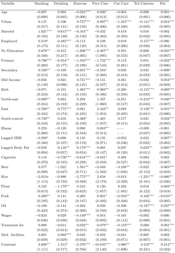
6.5 Health Input Coefficient Estimates: Male . . . 51
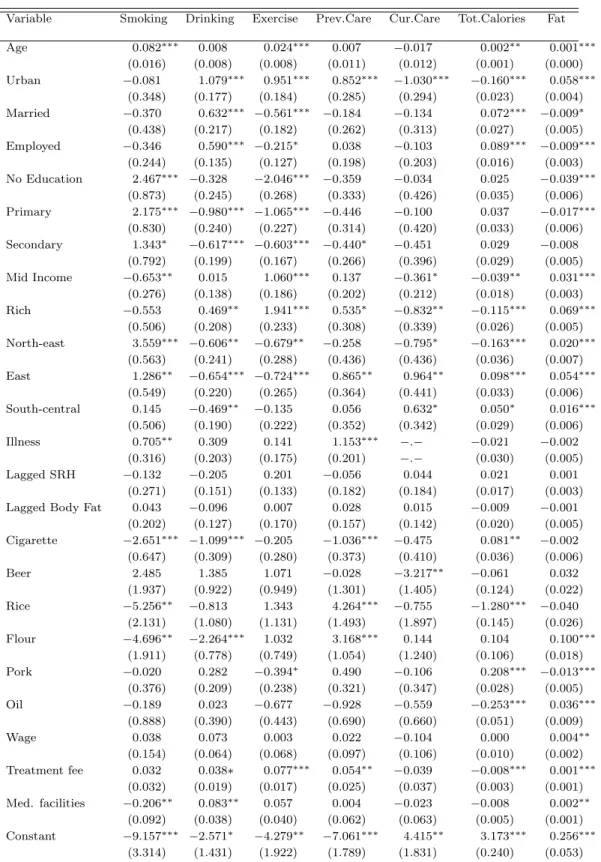
6.6 Health Input Coefficient Estimates: Female . . . 52
6.7 Health Input Marginal Effects: Male . . . 53
6.8 Health Input Marginal Effects: Female . . . 54
6.9 Model Fit . . . 55
7.1 Impact of a 40% Increase in Cigarette Price . . . 58
7.2 Impact of Low Cost Primary Medical Care . . . 61
A.1 Entry into estimation sample by wave . . . 67
A.2 Variation in Health Variables: Males . . . 67
A.3 Variation in Health Variables: Females . . . 68
A.4 Variation in Demographic Characteristics: Males . . . 69
A.5 Variation in Demographic Characteristics: Females . . . 70
A.6 Variation in Community Characteristics . . . 71
A.7 Variables . . . 72
LIST OF FIGURES
1.1 Trends in Adverse Health Outcomes in China . . . 3
3.1 Timing of the model . . . 14
5.1 Health Outcomes across Age . . . 40
7.1 Impact of Cigarette Price Rise on Smoking: Female . . . 59
7.2 Impact of Cigarette Price Rise on Drinking: Male . . . 59
7.3 Impact of Medical Treatment Fee Decrease on Preventive Care: Male . . 60
7.4 Impact of Medical Treatment Fee Decrease on Preventive Care: Female . 62 7.5 Impact of Smoking on Self-reported Health . . . 62
7.6 Impact of Exercise on Self-reported Health . . . 63
7.7 Impact of Exercise on Body Fat . . . 63
B.1 Model Fit: Self-reported Health . . . 74
B.2 Model Fit: Body Fat . . . 74
B.3 Model Fit: Smoking . . . 75
B.4 Model Fit: Fat Consumption . . . 75
Chapter 1
Introduction
Globally, non-communicable diseases are emerging as a leading cause of mortality, especially in low- and middle-income countries. Estimates from year 2008 indicate that non-communicable diseases (NCDs) accounted for 63 percent of the 57 million deaths worldwide. In addition to the mortality burden, projections have shown a 0.5 percent decrease in annual economic growth for every 10 percent increase in NCD prevalence (Alwan, 2010). Since these costs are largely preventable through low-cost interventions, there is an increased need to quantify the determinants of adverse health conditions and the contextual factors that influence these determinants. This paper estimates the impact of behavioral and medical health inputs on body fat and self-assessed health, along with reduced form estimates of the determinants of demand for each of these inputs. The analysis in this paper serves a twofold purpose. From the health production perspective, it attempts to quantify the effect of individual health input consumption and an illness shock on subjective and objective health measures. Furthermore, the reduced form demand equations capture the effects of local amenities and prices on input consumption laying the groundwork for eventually simulating the impact of price-based policies to encourage or discourage particular health behaviors that have sizeable marginal effects on health outcomes.
in the environments in which these individuals live. China serves as an interesting case study for the research question presented in this dissertation due to the rapid, large-scale transitions in the economy and population health patterns over the last few decades. As the most populous country in the world, China is no exception to the global trends in disease profiles and risk factors. As of 2008, the estimated prevalence rate of raised blood pressure is 38 percent among Chinese adults, while the overweight prevalence rate is 25 percent.1 Some of these adverse trends in health outcomes for the Chinese population are shown in Figure 1.1. While part of the worsening health outcomes can be attributed to age, it is clear that these trends exist among younger age groups as well. Several factors have contributed to the rising prevalence of chronic diseases in China. Since the 1980s, China has been experiencing rapid income growth and a decline in absolute poverty. These changes have been accompanied by increasing urbanization, and a shift in nutrition patterns towards energy-dense and high-fat diets. Moreover, rapidly occurring urbanization has also resulted in a decline in physical activity among Chinese adults (Ng, Norton, and Popkin, 2009). China is the largest producer and consumer of tobacco in the world. In 2010, China had an estimated smoking prevalence rate of around 53 percent for adult males. This rate was higher for men from rural areas and those without college education (Li, Hsia, and Yang, 2011). In spite of the rapid income growth, China continues to suffer from wide-spread inequality in income, limited availability of medical insurance, and unequal access to medical facilities. The dismantling of the rural communes in the late 1970s led to the collapse of the rural health care system. After the collapse of the old rural medical insurance scheme, there was no public health insurance scheme for rural residents until the recent introduction of the new cooperative insurance program. Thus, while the prevalence of chronic illnesses like hypertension and diabetes is on the rise, a large number of people go undiagnosed and/or untreated due to limited access to health care. All of these factors together imply that NCDs are potentially a
1WHO Report on non-communicable diseases, 2010
Figure 1.1: Trends in Adverse Health Outcomes in China
large burden on the public health system, and consequently on productivity and growth in China. Thus, the analysis of health behaviors of Chinese adults and the influence of these behaviors on their health outcomes hold valuable health policy insights.
if the assumed distribution of the unobservables does not reflect their true underlying distribution. In order to overcome this empirical challenge, I take a semi-parametric ran-dom effects estimation approach which models the unobservables across all the equations using an estimated discrete distribution. The estimates from this model are then used to simulate the effect of policy changes on health input demands and outcomes. These policy changes include an increase in the retail price of cigarettes and a decrease in the cost of seeking primary medical care.
Results from the estimation of the health production function indicate that exercise helps to increase the probability of reporting good health by over 2.5 percentage points for both men and women. In addition, exercise also has the beneficial effect of lowering body fat among women. Both smoking and drinking are harmful health inputs for women as they decrease the likelihood of reporting good health. Prices of cigarettes and alcohol could be useful tools for reducing the prevalence of undesirable behaviors. Both men and women are less likely to drink as cigarette prices increase, while women are also less likely to smoke when cigarettes become expensive. Men decrease alcohol consumption when faced with higher beer prices. The estimates from both the input demand and health production equations indicate that education is likely to induce participation in healthy behaviors such as exercising and seeking preventive care while simultaneously raising the consumption of dietary fat. The findings here are also consistent with previous work that indicates a shift to fat-based energy consumption with increase in wealth in China.
The remainder of the dissertation is organized as follows. Chapter 2 reviews the related knowledge to date and specifies the contribution of this dissertation. Chapter 3 discusses the theoretical model that motivates the empirical approach, and I describe the empirical method and identification strategy in Chapter 4. The data analysis sample are described in Chapter 5. Chapter 6 discusses the results from the estimation of the model. Policy experiments are described in Chapter 7, and Chapter 8 concludes.
Chapter 2
Background and Contribution
2.1
Related Literature
Health production functions have long been used in the health economics literature to quantify the determinants of individual health outcomes. The concept of health capital was formalized by Grossman (1972) in his seminal model in which individuals act as both consumers and producers of health. The production of health occurs through a health production function where health is determined by the consumption of medical care and other goods. In his model, health inputs act as investments that, along with the rate of depreciation of the health stock (δ), influence health outcomes. Since the publication of the Grossman model, a large body of empirical literature testing the the-oretical implications of the model has evolved. Moreover, in the last two decades several researchers have estimated empirical health production functions that attempt to capture the impact of health investments in the form of lifestyle behaviors like smoking, exercise and alcohol consumption. These production functions have been estimated for a wide variety of outcomes including self-rated health (Kenkel, 1995; Contoyannis and Jones, 2004), mortality (Balia and Jones, 2008), and obesity and weight gain (Rashad, 2006; Ng, Norton, Guilkey, and Popkin, 2012).
drink-of five health outcomes that include both subjective and objective health measures. Us-ing cross-section data from the National Health Interview Survey, he finds that excess weight, smoking and heavy drinking are detrimental across all measures of health. While Kenkel estimates health production functions for several outcomes, each of these equa-tions are separately estimated, thus not accounting for correlation between the various outcomes. Since health is a multi-dimensional phenomenon, it is reasonable to assume that these health outcomes are jointly produced and are correlated with each other. My work attempts to address this concern by jointly estimating two health outcomes along with a set of input equations, and allowing lagged values of both outcomes to affect current health inputs and outcomes.
While Kenkel recognizes the potential bias introduced by the endogeneity of health inputs, his attempt to use state-level prices as instrumental variables in a two-stage model does not yield plausible estimates as some coefficients have unexpected signs. For instance, stress is found to be beneficial to health in the two-stage models with prices. Kenkel attributes this discrepancy to the problem of weak instruments as state-level prices may not be good determinants of the demand for health inputs such as eating habits and stress. Building on Kenkel’s work, Contoyannis and Jones (2004) and Balia and Jones (2008) use the same set of health inputs to estimate the impact of lifestyles in mediating the relationship between self-rated health and mortality respectively. In order to correct for endogeneity, these papers estimate a joint system of health input and health outcome equations using a multivariate probit model that incorporates unobserved heterogeneity. Their methodology uses two waves of the British Health Panel Survey to estimate wave 2 health as a function of wave 1 lifestyles. One of the limitations in these analyses is the lack of contextual variables in explaining the choice of lifestyles. While individual characteristics are key determinants of input demand, the prices of and accessibility of said inputs also play an important role in the input demand functions. Other works have addressed this concern and successfully used input prices as instrumental variables.
Rashad (2006) uses cigarette taxes and restaurant prices as instruments in her estimation of the determinants of obesity using NHANES data. Employing longitudinal data from the China Health and Nutrition Survey, Ng, Norton, Guilkey, and Popkin (2012) use community-level prices of cigarettes, alcohol and several food items to identify the impact of diet, exercise, smoking, and drinking on the dynamics of weight among adult Chinese men. In order to account for the unobserved heterogeneity as well as the simultaneity of behaviors and weight dynamics, they use a Generalized Method of Moments framework with prices serving as identifying variables. They find that among Chinese males, 6.1 percent of the weight gain is caused by declining physical activity while about 3 percent can be attributed to nutritional decisions. My paper differs from that of Ng, Norton, Guilkey, and Popkin (2012) in that it incorporates an illness shock and medical care into the health production function. Moreover, my work focuses on two measures of health that are distinctly different from body weight. Finally, I use a semi-parametric random effects estimation strategy to account for the endogeneity of health inputs.
survey data from Vietnam to obtain elasticity estimates, and then use these estimates to analyze the implications financing alternatives to user fees for financing public healthcare. The China Health and Nutrition Survey with its longitudinal data on prices at the neighborhood level has been used for estimating the price effects of various goods that play an important role in determining individual health input choices. Guo, Popkin, Mroz, and Zhai (1999) estimate the elasticity of demand for six major food groups and find that large and significant price effects exist. Their model helps them identify path-ways for pricing policy to alter the fat intake of individuals, especially those in higher income groups. Lance, Akin, Dow, and Loh (2004) estimate the price elasticity of smok-ing among Chinese males. They find that the demand for cigarettes in the period from 1993 to 1997 is fairly inelastic, and that there may not be sufficient scope for pricing policy to alter cigarette consumption. However, their analysis does not control for the correlation between smoking and alcohol consumption. Accounting for the relationship between different goods allows for the empirical testing of the role of cross-price elasticity, which can have significant implications while testing the role of pricing policy in altering behavior.
2.2
Research Contribution
Through the research presented in this dissertation, I contribute to the economic liter-ature on health production by overcoming some of the previously discussed limitations, and incorporating additional features into the model. First, I model two health out-comes jointly - self-rated health and body fat measured using waist circumference. While health production functions that use either self-rated health (SRH) or body weight are commonly found in the literature, the simultaneous estimation of multiple health out-comes is not common in the economics literature.1 While, SRH is essentially a subjective
1Blau and Gilleskie (2001) model combinations of health outcomes to estimate the impact of health on employment transitions using a joint estimation technique.
an objective measure, such as this one, would also help me quantify the impact of policy changes on health in more meaningful terms.
Second, I include multiple health inputs in this model that include both medical care and lifestyle choices. While my model does not allow me to capture the structural parameters of the individual demand function for each of these inputs, it allows me to reduce the omitted variable bias that may result from excluding relevant health inputs from the health production equation. Additionally, modeling the endogenous demand for multiple inputs allows me to capture the correlation between these inputs (i.e., whether they are substitutes or complements). This will allow me to simulate more realistic policy experiments, where a change in a given health policy can affect outcomes via multiple pathways.
Third, the estimation of this model uses the semi-parametric discrete factor random effects estimation technique (Mroz and Guilkey, 1992). This is a more flexible estimation method in that it minimizes distributional assumptions on the joint error term. While (Contoyannis and Jones, 2004; Balia and Jones, 2008) estimate a similar system of equa-tions, they assume a multivariate normal distribution for the joint error term which allows them to use multivariate probit estimation. If the true distribution of the unobservables is indeed normal, then this assumption is not a problem. However, if the unobserv-ables are not normally distributed, this assumption could lead to biased estimates. In the estimation strategy employed in this paper, the distribution of the unobservables is approximated using a discrete step function. With this method, the distributional as-sumption is only restricted to the random component of the error term. This method has been shown to perform better than the usual maximum likelihood method when the true distribution of the error term is not normal (Guilkey and Lance, 2013). Moreover, unlike a multivariate probit model that requires all the dependent variables to be binary, the discrete factor method allows me to use both binary and continuous variables as dependent variables.
Chapter 3
Theoretical Motivation
This chapter outlines the economic theory underlying the demand for health inputs and the production of individual health. The model presented here is intended to provide a general theoretical background for the empirical analysis in this paper. The specific details of the variables to be used in estimation will be discussed in the chapter on the empirical model.
3.1
Model
The model discussed here is a simplified version of the model of insurance, health status, medical care and health behaviors used by Khwaja (2010). The approach in this work differs from Khwaja’s in that it does not model the decision to buy insurance. It is reasonable to believe that decisions regarding employment and insurance are endogenous with respect to the demand for health inputs as well as health outcomes. For instance, an individual who chooses to smoke might choose to buy health insurance as he recognizes that smoking is likely to have an adverse impact on his health. However, the focus of this paper is modeling the health production and input usage under the assumption that all other decisions are exogenously made.
evolves on the basis of the health shock he has faced and his input consumption.
3.1.1
Timing and Variables
Consider an individualiwho is observed forT periods. In each periodt, the individual has information about his demographic characteristics (Xit), income (Yit), previous period’s
perceived health stock (Hit−1), a lagged stock of measured body fat (Fit−1), allocation of
non-working time (Nit), community characteristics (Zt), and prices (pt). Decisions about
employment and work hours are not modelled in this paper. Therefore, non-working time is included as an exogenous variable. Demographic variables include age, gender, marital status, educational attainment and employment status. All of these variables are stacked in the vector Ωit. The individual’s information set at the beginning of period t can be
summarized as,
Ωit = [Hit−1, Fit−1, Xit, Yit, Nit, Zt, pt] (3.1)
At the beginning of period t, the individual observes a health shock rit, which is
described below. After observing the exogenous information and the health shock, he chooses how much medical care(mcit) to seek if he is sick. At the same time, he also makes decisions about alcohol consumption (ait), smoking (sit), physical exercise (eit), nutrition
(dit), and preventive medical care (mpit). At the end of period t, the health stocks are
updated to Hit and Fit, and the individual moves to the next period.
shock.
The timing of decision making for an individualiat timetis described by the following figure.
Figure 3.1: Timing of the model
-t−1 t t+ 1
Ωit
Observerit
Chooseait,sit,eit,git
mc itandm
p
it Hit, Fit
Ωit+1
In the theoretical model, I assume that individuals can choose to consume any non-negative amount of each of the goods. For estimation of the model, some of the variables are discrete, while others are continuous. This will be determined by the availability of data as discussed in the subsequent sections. For the rest of this section, the health behaviors are stacked into two vectors -bit denoting the non-medical inputs, andmit, the
medical care consumption. Thus, bit= (ait, sit, eit, cit, git) and mit = (mpit, mcit).
3.1.2
Health Shock and Health Transition
The individual enters every period with a state vector that includes a health shock rit,
which can be conceptualized as an episode of acute illness. The health shock can take one of two values,
rit =
1 if sick
0 if not sick
The probability of illness (λit = P(rit = 1)) depends on the health stock at the
beginning of the period and exogenous individual characteristics, and is given by,
λit =λ(Hit−1, Fit−1, Xit) (3.2)
The health inputs consumed by the individual, along with the health shock he faces at the beginning of the period, lead to the evolution of his health stocks Hit and Fit at
the end of period t. The health stock evolves according to a health production function that has inputs, the illness shock and prior health stock as arguments. It is assumed that a higher value of the health stock indicates that a person is in better health.
Hit=h(Hit−1, Fit−1, bit, mit, rit;Xit) (3.3)
Fit =f(Hit−1, Fit−1, bit, mit, rit;Xit) (3.4)
3.1.3
Utility, Constraints and Value Function
The individual gets utility from consumption (Cit), leisure (Lit), the health stocks at the
beginning of the period (Hit−1) and (Fit−1) and his consumption of health inputs (bit, mit).
The inclusion of medical inputs in the utility function can be viewed as the disutility an individual gets from having to visit the doctor or following the prescribed treatment. Thus, the consumption of health inputs has two impacts on the individual’s utility - a direct utility benefit (or cost) of consumption, and the indirect effect through the impact of the inputs on the health stock. Utility is also affected by exogenous characteristics (Xit) and an unobserved component (it), which act as preference shifters.
Uit=U(Cit, Lit, bit, mit;Hit−1, Fit−1, Xit, εit) (3.5)
Yit =Cit+pbtbit+pmt mit (3.6)
To model the time constraint, I assume that an individual has a per-period endowment of non-working time. Typically, hours spent working or on household production account for a large portion of an individual’s time. However, those decisions are not modeled in this paper. It is assumed that the time left over after paid work and/or household production is spent on leisure and health production.
Lit+mitNitm+eitNite =Nit (3.7)
In the equation above,Nitis the per period non-working time. The time spent seeking
medical care is denoted byNm
it. It is a vector that includes time spent on preventive and
curative care. Ne
itis the time spent on exercise. The time variables denote the time spent
per unit of input consumed, and are multiplied by the units of input to obtain the total time spent.
The two constraints are substituted into the utility function to obtain,
Uit=U(Yit−pbtbit−pmt mit, Nit−mitNitm−eitNite, bit, mit;Hit−1, Fit−1, Xit, εit) (3.8)
The agent’s value function, in a given period, from choosing a combination of medical and non-medical inputs {b, m} (i.e., bit =b and mit =m) in health state h, at body fat
level f, and with health shockr is
Vbmhf r(Ωit, it) =U(·) +δ
Z
h0
Z
f0
h
λit+1(h0, f0, X)Et[Vh
0f01
(Ωit+1)|dbmt = 1]
+ (1−λit+1(h0, f0, X))Et[Vh
0f00
(Ωit+1)|dbmt = 1]
i
dH(·)dF(·) (3.9)
where U(·) is described in (3.8), δ∈(0,1) is the discount factor, and
Vh0f0r0(Ωit+1) =Et
h
maxbm(Vh
0f0r0
bm (Ωit+1, εit+1) i
(3.10)
The expectation in equations (3.9) and (3.10) is taken over the unobserved preference shifter εit in the utility function.
The solution to the individual’s optimization problem, which involves choosing the alternative at each timet that maximizes lifetime utility, given information up to period
Chapter 4
Empirical Model
The theoretical model outlined in the previous chapter provides the motivation for the empirical model and strategy detailed here. In the theoretical model, the consumption of health inputs is modeled such that all input consumption decisions are simultaneously made. Similarly, the survey data used for empirical analysis asks individuals about their current consumption of multiple inputs such as cigarettes, alcohol and food. Thus, it is reasonable to assume that all decisions are jointly made, and hence all the input demand equations are estimated jointly. In addition, the health production equations are also modeled simultaneously with the input demand equations. The empirical specifications of the input demand and health production functions, obtained from the theoretical model of a forward-looking, utility maximizing individual, are modeled using a set of equations that is jointly estimated. This chapter describes the empirical strategy, the estimated equations, identification issues, and the technique adopted for dealing with sample attrition.
4.1
Estimation Strategy
such a system of simultaneous equations, it is common to make distributional assump-tions about this unobserved heterogeneity. However, if these distributional assumpassump-tions do not reflect the true distribution of the unobservables, the resulting estimates might be biased and inconsistent. In order to avoid the risk of biasing the model coefficients, I use a semi-parametric random effects estimation strategy that allows for greater flexibility in the distribution of the unobserved component. This estimation strategy is based on the Heckman-Singer (Heckman and Singer, 1984) approach that uses a discrete distribution to model the unobservable factors in a duration model. The discrete factor random effects method (Mroz, 1999; Mroz and Guilkey, 1992) used in this paper extends this approach to systems of equations that include both continuous and discrete dependent variables. This method allows for the modeling of heterogeneity at multiple levels. Thus, in the case of panel data, both permanent and time-varying heterogeneity can be modeled. For this purpose, the error term from the theoretical model, εit, can be decomposed into
three components,
εitj =µij +νitj+υitj (4.1)
where j denotes the jth equation, with the equations corresponding to the health
shock, input demand and health production functions, and j = 1,2, ...,12.
The unobserved component thus consists of time invariant individual heterogeneity (µij), time-varying heterogeneity (νitj) and an independently and identically distributed
component (υitj). The term (νitj) varies in each time period, but is correlated across the
equations for individuali. The permanent heterogeneity termµij is also correlated across
equations that will be described below. These components are allowed to be correlated across equations. Intuitively, the unobservable heterogeneity can be thought of as ‘types’ of individuals based on unobservable characteristics. The estimation technique accounts for the influence of these ‘types’ on individual demand for health inputs and the evolution of their health outcomes. The semi-parametric nature of this estimator comes from the distributional assumptions made for the term υitj. When the dependent variable is
bi-nary, this term is assumed to follow a Type I Extreme Value distribution. For continuous dependent variables, υitj is assumed to follow a Normal distribution.
4.1.1
Equations
Health Shock
The probability of facing an illness shock is a logit probability that depends on the individual’s exogenous characteristics1, the health status entering the period, and the
community illness vector Sit. This vector consists of two variables - the proportion of
people in the individual’s community, excluding the individual, who report communicable and non-communicable illness symptoms. Data on weather events or epidemics would be more suited to identifying the probability of illness. However, in the absence of such data, community illness variables serve as the best available option. The dependent variable is a binary variable that equals 1 if the individual reports being ill in the four weeks preceding the survey, and 0 otherwise.
ln
P r(rit= 1)
P r(rit= 0)
=τ0+Xitτ1+Sitτ2+Hit−1τ3 +BFit−1τ4+µ1i+ν1it (4.2)
1These are identical to the exogenous characteristics used in the input demand equations.
Health Inputs
There are seven health inputs in the model, which for theoretical convenience were stacked into two vectors bit and mit. Thus seven input demand equations are estimated - a logit
equation each for alcohol consumption (ait), smoking (sit), leisure physical exercise (eit),
preventive medical care (mpit) and curative medical care (mcit); and two equations for the continuous inputs - total calories consumed (cit) and proportion of fat in total energy
con-sumption (git). All inputs other than the two nutrition consumption inputs are modeled
as binary variables. In other words, individuals make a choice at the extensive margin. In case of medical care consumption, the CHNS asks individuals whether or not they seek medical care. There are some data on the total expenditure on medical care, but those variables have several missing values. In addition, expenditure could be largely in-fluenced by where individuals live, and whether or not they have any medical insurance.2 In addition, medical care consumption is modeled as being conditional on the individual reporting illness as data on curative medical care are only available for individuals who report having been ill. The calorie and fat consumption variables are allowed to be con-tinuous variables instead of imposing arbitrary thresholds for what might be healthy or unhealthy diets. Fat consumption is measured as a ratio of calories consumed from fat to total calorie consumption. The dependent variable is thus a continuous variable that takes values between 0 and 1.
Each of the health input demands is a function of the individual’s demographic and socio-economic characteristics (Xit), the health variables coming into the period
(Hit−1, Fit−1), the current period health shock (rit) and a vector of other exogenous
char-acteristics (Zit) that describe the factors in the individual’s environment. TheX vector
includes age, education, marital status, employment status, household income status,
and urban/rural residence. It also includes indicators for the region the individual lives in. The nine provinces covered in the survey are divided into four regions based on the geographic area they are located in. One important component of demographic char-acteristics is the number of children an adult has. It is reasonable to expect that the number of children a woman has bears an important influence on her health behaviors as well as health outcomes, especially body fat. However, number of children cannot be considered an exogenous variable as it is likely to be influenced by the woman’s health behaviors and outcomes. Thus, accounting for the number of children in this analysis will require modeling a woman’s decision to have children. In order to limit the scope of the research question in this dissertation, the number of children a woman has is excluded from the analysis. Gender is not included in the X vector. Given the observed gender differences in the choice of health behaviors, it is more appropriate to estimate separate models for males and females. This approach is important if the effect of unobservable characteristics on input demand varies by gender. The Z vector consists of prices and community infrastructure characteristics. The details of the variables included in the Z
vector are discussed in the following sub-section.
Instead of using measured individual or household income as an explanatory variable, this paper uses an income status variable that is based on a wealth index constructed using data on household infrastructure and household ownership of durable assets. Household wealth categorization based on such an index has been shown to be significantly correlated with income categories based on household expenditure (Filmer and Pritchett, 2001). An advantage to using such a wealth index is that it provides a measure of a household’s permanent living standards, and is less likely to be influenced by transitory health status, health behaviors or income. The construction of this asset index is described in the data chapter.
The health input demand equations do not model addiction by accounting for lagged input usage, although it is fair to assume that there may be some habit persistence in
behaviors. This characteristic may be especially true for smoking and drinking. However, using lagged inputs would restrict my sample size, and would require joint estimation of additional initial condition equations, adding to an already large system of equations. It is therefore assumed that the impact of lagged inputs only affects current behaviors through lagged health outcomes. That is, conditional on health and body fat entering the period, lagged behaviors have no independent effect on current behaviors.
Since the input equations are estimated simultaneously, they are all functions of the same exogenous variables. The estimated equations are as follows.
Alcohol Consumption
ln
P r(ait = 1)
P r(ait = 0)
=α0+Xitα1 +Hit−1α2+Fit−1α3+Zitα4+ritα5+µ2i+ν2it (4.3)
Smoking
ln
P r(sit= 1)
P r(sit= 0)
=β0+Xitβ1+Hit−1β2+Fit−1β3+Zitβ4+ritβ5+µ3i+ν3it (4.4)
Exercise
ln
P r(eit= 1)
P r(eit= 0)
=θ0+Xit−1θ1+Hit−1θ2+Fit−1θ3+Zitθ4+ritθ5+µ4i+ν4it (4.5)
Calorie Consumption
cit =ξ0+Xitξ1+Hit−1ξ2+Fit−1ξ3+Zitξ4+ritξ5+µ5i+ν5it+υ5it (4.6)
Fat Consumption
Preventive Care
ln
P r(mpit= 1)
P r(mpit= 0)
=φ0+Xitφ1+Hit−1φ2+BFit−1φ3+Zitφ4+ritφ5+µ7i+ν7it (4.8)
Curative Care
ln
P r(mc
it= 1)|P r(rit = 1)
P r(mc
it= 0)|P r(rit = 1)
=ψ0+Xitψ1+Hit−1ψ2+BFit−1ψ3+Zitψ4+µ8i+ν8it (4.9)
Health Outcomes
There are two health outcome equations - one for self reported health, and the other for body fat. Self-reported health is a binary variable that equals 1 if individuals report good health and 0 if they report poor health. Body fat is measured using waist circumference which is a continuous variable. In the empirical health production equations, health is a function of lagged health outcomes, the health shock, and contemporaneous input consumption. The health shock is also included in the equation to capture the effects of the shock that may not be reflected through the input demands. The equation includes the same X vector as for all the previous equations, excluding income status. The Z
vector is, however, excluded from the health outcome equation as those variables are assumed to affect health only through their impact on the health behaviors.
Self-rated Health
Hit=
0 if poor or fair
1 if good or excellent
ln
P r(Hit= 1)
P r(Hit= 0)
=γ0+Hit−1γ1+Fit−1γ2+bitγ3+mitγ4+Xitγ5+ritγ6+µ9i+ν9it (4.10)
Body Fat
Fit=ζ0+Hit−1ζ1 +Fit−1ζ2+bitζ3+mitζ4+Xitζ5+ritζ6+µ10i+ν10it+υ10it (4.11)
4.1.2
Identification and Initial Conditions
The equations described above are simultaneously estimated as a set of equations with the endogenous health inputs being the explanatory variables in the health outcome equa-tions. In order for this system to be identified, valid exclusion restrictions are necessary. I use community level characteristics to identify the demand equations. It is plausible to assume that these variables only affect an individual’s health through their impact on his health behaviors. Since the equations are all estimated simultaneously, the same exclusion restrictions are used in each of the input demand equations. While the com-plete system of equations is identified by the order condition,3 I present a justification for the different variables that are used as exclusion restrictions and how they potentially contribute to the identification of the set of equations.
The prices of a pack of local cigarettes and a bottle of local beer are included as they can be assumed to directly influence individual decisions to smoke and consume alcohol. Rice, noodles, pork and the most commonly used edible oil are among the basic food items that account for both total calorie consumption and fat consumption. The prices of these four goods are therefore included in the exclusion restrictions.4
There are no prices available in the data that could affect the decision to engage in physical exercise. However, I assume that the decision to exercise is influenced by two factors - access to exercise facilities, and the opportunity cost of time. Thus, the exclusion
3The order condition for identification requires that the number of exclusion restrictions is at least as much as the number of endogenous variables, less one.
restrictions include the wage for an unskilled worker in the neighborhood (separate for males and females). The theoretical model includes a time constraint for exercise. Here I use wages as a proxy for the time constraint, in an attempt to capture the opportunity cost of time. Data on access to exercise facilities are not available for the entire sample period and are therefore excluded from the analysis in this paper.
The decision to seek medical care, whether preventive or curative, depends on the ease of accessing clinics and hospitals. With limited access to health insurance in China over the sample period, medical care often involves high out of pocket expenditures. However, in the survey, expenditures are observed only for individuals who seek medical care. Other factors that may influence the decision to seek care are the time and money cost of traveling to a facility and the availability of medical insurance programs provided by the government. On the basis of data availability and quality, I use the average treatment fee for an episode of acute illness and the number of medical facilities within the community as exclusion restrictions.5
In this dissertation, a health shock is defined as an episode of illness, and is primarily used to account for selection into seeking medical care. Episodes of illness can be in-fluenced by many factors such as weather, pollution and the prevalence of a contagious illness in the neighborhood. In the absence of data on weather and pollution, I use a constructed measure of community-level illness in order to identify the health shock equa-tion. Two measures are constructed - one for the proportion of people in the individual’s community who report an acute illness shock, and the other for the proportion reporting a chronic health shock.6
5This cost is computed as a community-level average of household reported treatment costs at medical facilities. These costs come from a general household survey of medical facilities, and not the price that a household paid for treatment in the past month.
6The measures are based on the reporting of health shocks in an individual’s community, excluding the individual himself.
The estimation equations specify current health outcomes as a function of contem-poraneous inputs and lagged health measures. There are no lagged health outcomes to estimate health status in the first wave for each individual. Thus, I also estimate ini-tial conditions for the two health outcomes. Iniini-tial health is modelled as a function of individual exogenous characteristics such as age, education, employment, marital sta-tus, and income status. Exogeneous community-level characteristics such as prices and community infrastructure are also used in the initial health equations. The exclusion restrictions that help identify initial health are height and exposure to the Great Famine, either in-utero or as a child, or being born immediately following the end of the famine.7
4.1.3
Likelihood Function
As mentioned earlier, the set of equations specified above is estimated using a semi-parametric maximum likelihood method which approximates the distribution of unob-served heterogeneity using mass points and the probability associated with those mass points. The method estimates K mass points for µand G mass points for νt. The
prob-ability ρk is associated with the kth permanent mass point µk and ωg is associated with
the gth time-varying mass point νgt. In order to ensure identification of the mass points
and probabilities, the coefficients of the first permanent and time-varying mass points are normalized to zero. In addition, the probabilities are restricted to sum to one.
The unconditional contribution of individual i to the likelihood function is,
li(Θ, ρ, ω) = K X k=1 ρk ( 1 Y h=0
P r(Hi1 =h|µ11k)1[Hi1=h]
1
σφ(Fi1|µ12k)
T Y t=2 ( G X g=1
ωg(Bg)
))
(4.12) where
Bg =
1 Y
r=0
P r(rit =r|µ1k, ν1gt)1[rit=r]
1 Y
a=0
P r(ait=a|µ2k, ν2gt)1[ait=a]
1 Y
s=0
P r(sit=s|µ3k, ν3gt)1[sit=s]
1 Y
e=0
P r(eit =e|µ4k, ν4gt)1[eit=e]
1
σφ(cit|µ5k, ν5gt)
1
σφ(git|µ6k, ν6gt)
1 Y
mp=0
P r(mpit =mp|µ7k, ν7gt)1[m
p it=mp]
1 Y
mc=0
P r(mcit =mc|µ8k, ν8gt)1[m
c
it=mc]1[rit=1]
3 Y
h=0
P r(Hit=h|µ9k, ν9gt)1[Hit=h]
1
σφ(Fit|µ10k, ν10gt) (4.13)
The estimated joint probability, ρk, of the kth permanent mass point vector is given
by equation (4.14), while the estimated joint probability of the gth time-varying mass
point (ωg) vector is described in equation (4.15).
ρk =P r(µ1 =µ1k, µ2 =µ2k, µ3 =µ3k, µ4 =µ4k, µ5 =µ5k, µ6 =µ6k
µ7 =µ7k, µ8 =µ8k, µ9 =µ9k, µ10=µ10k, µ11 =µ11k, µ12=µ12k)
(4.14)
ωg =P r(ν1 =ν1g, ν2 =ν2g, ν3 =ν3g, ν4 =ν4g, ν5 =ν5g, ν6 =ν6g
ν7 =ν7g, ν8 =ν8g, ν9 =ν9g, ν10=ν10g)
(4.15)
The joint likelihood function over all the individuals is
L(Θ, ρ, ω) =
N
Y
i=1
li(Θ, ρ, ω) (4.16)
where Θ is the entire set of parameters estimated, i.e., Θ = (α, β, θ, ξ, η, φ, ψ, τ, γ, ζ). Thus, we have a joint likelihood function for the entire sample. The DFRE method
integrates over the distribution of the unobserved heterogeneity, and the parameters Θ,
ρ and ω are estimated simultaneously.
4.2
Attrition
The dataset used for estimating this model is an unbalanced panel dataset where some individuals are followed through the entire survey period, while others are lost to follow up after a few years. In addition, new individuals are added over time to replenish the survey sample. This attrition implies a possible source of bias in the estimated coefficients. The method of selecting the analysis sample for this paper introduces an additional source of attrition bias. Since the sample is restricted to individuals with complete data on all dependent variables, missing data on any one of these variables results in exclusion of the individual from the analysis sample. In this analysis, attrition is an absorbing state so that individuals who exit the sample in any year are not allowed to re-enter the sample. This is done in view of the time lapse between consecutive survey waves, which range from two to four years. If individuals in the sample are allowed to skip waves, it may create a very long time gap between their lagged health outcomes, and current health inputs and outcomes. This could potentially lead to weaker explanatory power of the lagged variables across all the equations.
pit≡πi2πi3. . . πit (4.17)
In this equation, the π terms are the fitted probabilities for individual i in each period, while pit is the probability used to construct the final attrition weight. The
attrition weight is simply an inverse of the probability pit.
Chapter 5
Data and Sample Characteristics
5.1
Data
The data used for the empirical analysis are from the China Health and Nutrition Survey (CHNS), which is a longitudinal survey conducted and maintained by the Carolina Popu-lation Center at the University of North Carolina at Chapel Hill along with the National Institute of Nutrition and Food Safety at the Chinese Center for Disease Control and Pre-vention.1 The goal of the survey is to study health, nutrition and family planning policies
in China. The first round of the survey was conducted in 1989 and subsequent rounds of data collection occurred in 1991, 1993, 1997, 2000, 2004, 2006, 2009 and 2011. In addition to information on individuals and the households they live in, the CHNS fields a community survey to collect data on community infrastructure, demographics and prices of commonly consumed goods. The CHNS sample is drawn from nine provinces of China (Guangxi, Guizhou, Heilongjiang, Henan, Hubei, Hunan, Jiangsu, Liaoning, and Shandong). These provinces are very diverse in terms of socio-economic, health and demographic measures. A multistage, random cluster selection process was used to
draw the study sample in each province. Within each province, counties were strati-fied by income, and random sampling was used to select counties. Villages, towns and urban neighborhoods were then selected from among these counties. At the individual level, detailed data about demographics, income, insurance coverage, medical care uti-lization, diet, and measures of health are available. The CHNS surveys households about income, household assets and availability of medical care facilities. The community sur-vey includes information on community infrastructure, health services, family planning services, prices, wages and population characteristics.
The CHNS is not a balanced panel as some individuals and households leave the survey over time, and new households are added to replace the ones that leave. In addition, members from survey households who establish a new household have also been added to the survey since 1993. An additional source of survey attrition comes from the fact that Liaoning province could not be surveyed in 1997 due to floods in Liaoning in that year, and was dropped from the sample. Another province from the same region, Heilongjiang, was included in the sample instead. In year 2000, Liaoning returned to the survey and both provinces have been retained in the survey ever since2.
5.2
Sample Selection
This paper uses data from the 1997 to 2006 waves of the CHNS. The choice of survey waves is motivated by the availability of data on the variables of interest. Prior to 1997, individuals were not asked about leisure physical activity. In addition, the survey questions are more consistent across waves starting in 1997. Individuals were not asked about reported health in the 2009 survey. Since the current analysis includes self-reported health as one of the health outcomes, observations from the 2009 wave will have to be excluded from the sample.
2The analysis sample in this paper does not restrict the year of entry to any specific survey wave. This allows me to use individuals from all provinces in the sample.
Health in each period is a function of input demands from the previous period. Also, input demands in a given period are themselves influenced by the individual’s health when entering the time period. Finally, since ‘prior’ health is controlled for, an initial condition equation has to be estimated for the first period an individual is observed. For all of these reasons, only individuals with complete data on health inputs and outcomes for two or more waves are included in the estimation sample. This implies that individuals can be in the sample for two, three or four consecutive waves. In addition, disabled individuals and women who report being pregnant during the survey period are excluded from the sample for that survey year. The final selection restriction is that only adults between the ages of 18 and 60 are included in the sample. The sample selection rules do not require all individuals to enter the sample in the same period. Thus, the year of entry into the sample varies across individuals. About half the sample is first observed in 1997 while about 23 percent is first observed in 2000. The remaining individuals first enter the sample in 2004. Since 2006 is the last year individuals are observed in, no one enters the sample in 2006.
After applying all the selection rules, the final estimation sample consists of 18,302 person-wave observations on 6601 unique individuals. These observations have complete data on all the dependent variables of interest, namely health behaviors and health out-comes. Some of these observations have missing data on income status and community-level covariates. Instead of imputing the values of these variables, the estimation equa-tions include indicators for missing data wherever applicable.
5.2.1
Attrition
not observed in 2004.
Among males, about 23 percent of the sample in year 2000 is observed attriting while the corresponding number for year 2004 is 20.5 percent. The female sample has a slightly lower attrition rate with 21 percent of the observed sample exiting at the end of year 2000 and 16 percent at the end of 2004. Overall, 11.4 percent of the total observations attrit the sample at some point.
Table 5.1: Attrition: Males Year Attrit Not Attrit Total
1997 0 1622 1622
2000 538 1779 2317
(%) 23.22 76.78
2004 535 2064 2599
(%) 20.58 79.42
2006 0 2064 2064
Table 5.2: Attrition: Females Year Attrit Not Attrit Total
1997 0 1766 1766
2000 547 2026 2573
(%) 21.26 78.74
2004 473 2444 2917
(%) 16.22 83.78
2006 0 2444 2444
This observed sample attrition may bias the estimated coefficients if the probability of leaving the sample depends upon an individual’s health outcome or health behaviors. For example individuals who are in poor health may be relatively difficult to locate or unusually reluctant to answer questions about exogenous characteristics like age, educa-tion or income level. The estimaeduca-tion strategy adopted in this paper accounts for such
potential sources of bias, as discussed in the chapter on the empirical strategy.
5.3
Asset Index
The estimation equations used in the analysis presented in this work include, as a part of individual characteristics, a measure of wealth based on a household asset index.The CHNS does include data on current household income from several different sources. However, current income could be influenced by individuals’ current health status. More-over, current income is subject to temporary fluctuations and may not be a true measure of long term economic status. A measure of wealth based on an asset index helps circum-vent these problems. This asset index is calculated according to the approach described in Filmer and Pritchett (2001) for constructing a single measure of household wealth status on the basis of asset ownership questions that are commonly asked in survey data sets.
capture a large amount of the variation in the data3. The predicted score based on the
first principal component is used as the asset index. Further, deciles of the distribution of the score index are obtained and households are classified as poor, middle-income and high-income (rich) based on their position in the decile distribution. Households in the bottom four deciles are classified as poor, the top two deciles are classified as rich, and the rest are middle-income.
In order to test whether the wealth status indicator based on the asset index is a good proxy for measured income status, it is compared to an indicator of wealth status based on the household income data from the CHNS. The decile distribution of the gross annual household income is used to construct variables denoting poor, middle income and rich households based on income. The income-based indicator for each category is found to be strongly positively correlated with the corresponding indicator based on the asset index and negatively correlated with the other categories. Thus, the asset-index based wealth status constructed in this paper can be assumed to be a good proxy for household income status.
5.4
Sample Description
Table 5.3 describes the demographic information for the estimation sample, while Ta-ble 5.4 shows the prevalence of health behaviors and outcomes. In these taTa-bles the summary statistics are pooled across all the waves and observations. In addition, the characteristics of the male and female samples are described separately as the empirical model is estimated separately by gender. The appendix includes tables for each wave of data in order to show the variation in the data through time.
In the case of both males and females, almost a third of the sample lives in urban areas. Almost 87 percent of male observations and 91 percent of female observations
3It is standard practice for studies based on DHS data sets to use only the first component from the PCA to construct asset indices.
report being currently married. Divorced, widowed and never married individuals are grouped together in the not married category. There is a marked difference in educational attainment by gender. Among males, 8 percent of observations report having little to no formal education, while almost 60 percent have completed secondary education. In contrast, half of the female sample has completed primary education or less. A closer look at the data reveals a generally increasing trend in educational attainment among females over the years. The average per capita household income over the sample period is 6790 yuan for males and 6748 yuan for females. These incomes are adjusted to the CPI for year 2006. Around 45 percent of the sample is middle income, while around 15 percent is in the high-income (rich) category.
Table 5.3: Means of Demographic Characteristics
Variable Male Female
Age 41.89 42.36
(10.36) (9.62)
% Urban 31.93 32.11
% Married 86.66 91.19
% Employed 85.2 71.60
Education
% None 8.16 25.48
% Primary 22.01 23.77
% Secondary 59.25 42.69
% Higher Ed 10.58 8.05
Average yearly income 6790.51 6760.18 ( 8351.99) (8443.06) Asset index based
% Poor 39.08 38.72
% Middle Income 45.61 46.83
% Rich 15.31 14.45
Standard deviation in parentheses.
Income is per capita gross household income in 2006 yuan.
In contrast, only 3 percent of the female sample reports currently smoking and under 10 percent reports any drinking. While a very small proportion of the sample reports seeking preventive care, the figure is higher in the female sample by almost a percentage point. Similarly, a higher proportion of women seek curative care, both unconditionally and conditional on reported illness. Both men and women consume similar amounts of dietary fat, with the average for the female sample being slightly higher.
A higher proportion of the male sample reports being in excellent or good health than the female sample. The average waist circumference for men is 81.37 cm, which is a little above the cut-off of 80 cm (for adult men and women in China) beyond which the risk of cardiovascular disease increases (Wildman, Gu, Reynolds, Duan, and He, 2004). The average waist circumference for the female sample is smaller and below the cut-off at 78 cm.
Figure 5.1 shows the means of the two health outcomes by age group for the pooled sample. As men and women age, their probabilities of reporting good health decrease dramatically. While around 80 percent of each sub-sample reports good health in the 20 to 30 age group, the number falls to 60 and 50 percent, for men and women respectively, when their age goes above 50. The graph shows the proportion of the sample whose waist circumference is greater than 80 centimeters. The proportion steadily increases over age groups, with the rise being more pronounced for women.
The trends over time shown in the appendix tables (see Tables A.2 and A.3) reveal interesting data patterns. Over time, leisure physical activity has been declining for men and increasing for females. Consumption of dietary fat has steadily increased through 2004 with a small drop off in consumption for both genders in 2006. However, this appears to be an anomaly in the data set as there is an increase in fat consumption from 2006 to 2009.4 There is a sharp increase in the use of both types of medical care in the
year 2004. This could possibly correspond with the introduction of the new rural medical
4This pattern is observed in the survey data set and not just the estimation sample in this analysis.
Table 5.4: Health Inputs and Outcomes: Means
Variable Male Female
N 8602 9881
Inputs
% Smoke 61.68 3.16
% Drink 65.83 9.54
% Exercise 12.26 6.88
% Preventive Care 1.49 2.19 % Curative Care 5.95 8.21 % Curative Care if sick 61.68 66.32 Total calories per day 2529.61 2181.25
(723.93) (656.87) % Energy from fat per day 27.43 28.55 % Report Illness 8.01 9.98
Outcomes
% Good Health 72.56 65.07
Waist circumference 81.37 78.05 (centimeters) (9.55) (9.09) Standard deviation in parentheses.
insurance program in China. As the sample ages, individuals report worse health and higher body fat as measured by waist circumference.
The characteristics of the survey communities that sample individuals live in are described in Table 5.5. As with the household variables, the community variables also suffer from a missing data problem. In addition, some infrastructure related information such as availability of gyms, parks, and insurance plans, was only collected in the later waves of the survey.5
Figure 5.1: Health Outcomes across Age
Table 5.5: Community Characteristics Variable Full sample N
Local cigarettes 3.75 18216 (yuan per pack) (2.35)
Local beer 2.28 18216
(yuan per bottle) (0.77)
Pork 14.86 18216
(yuan per kg) (3.38)
Edible oil 7.93 18216
(yuan per liter) (1.87)
Rice 2.64 18216
(yuan per kg) (0.67)
Flour 3.12 18216
(yuan per kg) (0.77)
Wage: male 26.03 16876
(yuan) (13.80)
Wage: female 20.43 16640
(yuan) (8.93)
Medical facilities 2.83 16853 (Number in community) (1.49)
Avg treatment cost 41.83 17771
(yuan) (33.84)
Standard deviations in parentheses.
Prices and costs in yuan adjusted to 2006 prices.
Chapter 6
Results
This dissertation describes a model of health production with jointly estimated equa-tions for smoking, drinking, exercise, medical care consumption, calorie consumption, self-reported health and body fat. In this chapter, I present the results from the model estimated using the Discrete Factor Random Effects method. The coefficient estimates for the illness shock equation and the heterogeneity parameters are presented in Appendix B.
6.1
Health Outcomes
Table 6.1 shows the coefficient estimates and marginal effects from the health production equations for the male sub-sample. Exercise is a beneficial health input as it improves the likelihood of reporting good health and also results in a lower measure for waist cir-cumference (the proxy for body fat). Exercising leads to a 2.3 percentage point increase in the probability of reporting good health and this effect is significant at the 10 per-cent level of significance. The beneficial effect of exercise on body fat is, however, not statistically significant and therefore indistinguishable from zero.1
Table 6.1: Health Production Estimates: Male
Variables Good Health Body Fat
Coefficient Marginal Effect Coefficient Marginal Effect
Smoking 0.085 0.010 −0.055 −0.055
(0.138) (0.045)
Drinking 0.060 0.007 0.015 0.015
(0.098) (0.028)
Exercise 0.204∗ 0.023 −0.015 −0.015
(0.111) (0.028)
Preventive Care −0.336 −0.044 0.161∗∗ 0.161
(0.282) (0.068)
Curative Care −0.175 −0.022 −0.01 −0.010
(0.209) (0.063)
Total Calories 0.289∗∗∗ 0.035 0.032 0.032
(0.080) (0.020)
Fat −0.359 −0.040 0.243∗∗ 0.243
(0.424) (0.120)
Illness −1.531∗∗∗ −0.260 −0.028 −0.028
(0.162) (0.050)
Lagged SRH 0.728∗∗∗ 0.098 0.061∗∗∗ 0.061
(0.077) (0.023)
Lagged Body Fat 0.065∗ 0.008 0.677∗∗∗ 0.677
(0.037) (0.014)
Age −0.031∗∗∗ −0.004 0.001 0.001
(0.004) (0.001)
Urban −0.361∗∗∗ −0.045 0.008 0.008
(0.076) (0.020)
Married 0.157 0.02 0.098∗∗∗ 0.098
(0.110) (0.031)
Employed 0.054 0.006 −0.046∗ −0.046
(0.088) (0.026)
No Education −0.507∗∗∗ −0.069 −0.152∗∗∗ −0.152
(0.154) (0.042)
Primary −0.402∗∗∗ −0.052 −0.096∗∗∗ −0.096
(0.131) (0.034)
Secondary −0.182 −0.022 −0.058∗∗ −0.058
(0.114) (0.029)
North-east 0.402∗∗∗ 0.046 0.222∗∗∗ 0.222
(0.124) (0.033)
East 0.440∗∗∗ 0.050 0.209∗∗∗ 0.209
(0.128) (0.034)
South-central −0.054 −0.006 0.125∗∗∗ 0.125
(0.109) (0.029)
Constant 1.300 − 1.746∗∗∗ 1.746
(0.815) (0.221)
Significance: * p<0.1, ** p <0.05, *** p <0.01 Higher education, South-west are the omitted categories. Standard errors in parentheses.
waist circumference. While the magnitude of the effect, after controlling for other health inputs, is small, the effect is certainly in the expected direction. The results show that individuals who seek preventive care have higher levels of body fat. This result could potentially be driven by individuals with lower body weight and fat who experience an increase in waist circumference as a result of seeking preventive care.2
As men grow older, they report poorer health even after controlling for prior health. Age, however, has no impact on body fat. People with higher lagged body fat have a bigger waist circumference in the current period. Higher body fat also seems to lead to a higher probability of reporting good health in the future. This is consistent with the perception in China that excess fat is an indicator of greater wealth and well-being (Wu, 2006; Tang, Yu, Du, Ma, Zhu, and Liu, 2010). Men in the east and north-east region have a high probability of reporting good health relative to those in south-west China. The eastern region includes the province with the highest income in the country. Thus, the increased probability of good health could potentially reflect a better quality of life. Finally, men with lower levels of education have a lower probability of reporting good health, and less body fat relative to men who have completed higher education.
The coefficients from the health production equations for females are shown in Ta-ble 6.2. Exercise is beneficial to both subjective and objective health as it leads to a 0.7 centimeter decrease in waist circumference and a 2.2 percentage point increase in the probability of reporting good health. However, these effects are only significant at the 10 percent level of significance. As with men, an illness shock reduces the probability of reporting good health among women. Smoking and drinking significantly reduces the probability of reporting good health among women, by 5 and 4 percentage points respec-tively. Current body fat is increasing in both previous body fat and previously reporting good health. Controlling for consumption of dietary fat and lagged body fat, total calorie
consumption leads to lower body fat among women.
Urban women are likely to report significantly poorer health. Older women also report poorer health, but they also seem to have increased body fat although the magnitude of the effect is very small. While men with lower education have lower body fat, the opposite seems to be true for women. Relative to women who have completed higher education, those with lower levels of education have larger waist circumferences. One hypothesis that explains this result could be that women with higher education tend to exercise more and eat healthier, thus resulting in lower body fat. The switch in the impact of education on body fat across genders is certainly puzzling, and could merit further analysis that could incorporate the differences in health knowledge by levels of education.3
6.1.1
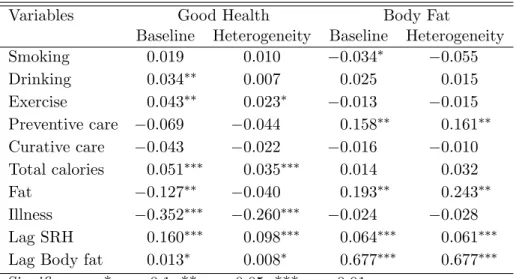
Comparing Estimates across Models
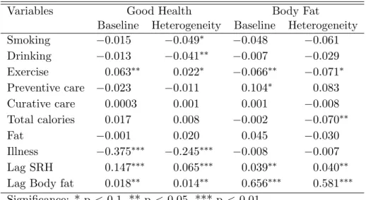
Tables 6.3 and 6.4 compare marginal effects from the preferred specification with het-erogeneity to the baseline model that does not incorporate unobserved hethet-erogeneity. The direction of bias in the model without heterogeneity depends on correlation between unobservable factors, health inputs and outcomes. For instance, women who experience stress may be more likely to smoke and drink, and less likely to report feeling good about their health. This would result in a downward bias in the marginal effect of smoking and drinking on self-reported health as observed below. The size and direction of the bias in marginal effects varies across all the outcome equations and the two sub-samples. For the male sub-sample, the marginal effects in the equation for self-reported health show a clear upward bias in the model without unobserved heterogeneity. No such clear bias is observed in the marginal effects for body fat. Similarly, there is no clear direction of bias in the coefficients from the model without unobserved heterogeneity for the female
3The CHNS contains some data on diet and activity knowledge in the later waves of the survey. These could be incorporated in an analysis of health production among women.