Quantum-enhanced metrology with the single-mode coherent states of an optical cavity inside a quantum feedback loop

states of an optical cavity inside a quantum feedback loop

.

White Rose Research Online URL for this paper:

http://eprints.whiterose.ac.uk/106377/

Version: Accepted Version

Article:

Clark, LA, Stokes, A and Beige, A orcid.org/0000-0001-7230-4220 (2016)

Quantum-enhanced metrology with the single-mode coherent states of an optical cavity

inside a quantum feedback loop. Physical Review A, 94 (2). 023840. ISSN 1050-2947

https://doi.org/10.1103/PhysRevA.94.023840

© 2016 American Physical Society. This is an author produced version of a paper

published in Physical Review A. Uploaded in accordance with the publisher's self-archiving

policy.

[email protected] https://eprints.whiterose.ac.uk/ Reuse

Unless indicated otherwise, fulltext items are protected by copyright with all rights reserved. The copyright exception in section 29 of the Copyright, Designs and Patents Act 1988 allows the making of a single copy solely for the purpose of non-commercial research or private study within the limits of fair dealing. The publisher or other rights-holder may allow further reproduction and re-use of this version - refer to the White Rose Research Online record for this item. Where records identify the publisher as the copyright holder, users can verify any specific terms of use on the publisher’s website.

Takedown

If you consider content in White Rose Research Online to be in breach of UK law, please notify us by

of an optical cavity inside a quantum feedback loop

Lewis A. Clark, Adam Stokes, and Almut Beige

The School of Physics and Astronomy, University of Leeds, Leeds LS2 9JT, United Kingdom (Dated: July 25, 2016)

In this paper, we use the non-linear generator of dynamics of the individual quantum trajectories of an optical cavity inside an instantaneous quantum feedback loop to measure the phase shift between two pathways of light with an accuracy above the standard quantum limit. The feedback laser provides a reference frame and constantly increases the dependence of the state of the resonator on the unknown phase. Since our quantum metrology scheme can be implemented with current technology and does not require highly-efficient single photon detectors, it should be of practical interest until highly-entangled many-photon states become more readily available.

PACS numbers: 06.20.-f, 03.67.Ac, 42.50.Lc, 42.50.Ar

I. INTRODUCTION

In general, there are two main strategies for reducing the uncertainty in an experimentally measured quantity. One method is to repeat the experiment many times. Another is to use more of an appropriate resource, N, in every run of the experiment. However, increasing N

is not always possible. Suppose we want to measure the phase shiftϕcaused by a delicate material with the help of a standard light interference experiment. Increasing the number of photons passing through can increase the accuracy of every phase measurement but also limits the lifetime of the sample [1–3]. In this case, it is impor-tant that every run of the experiment is as accurate as possible. To allow for a fair comparison of different mea-surement schemes, the error propagation formula

∆ϕ = ∆M

∂M ∂ϕ

(1)

can be used to calculate the accuracy ∆ϕof a given signal

M(ϕ) [4]. Here ∆M denotes the uncertainty (or resolu-tion) of M, while the visibility, |∂M /∂ϕ|, tells us how sensitiveM is to changes inϕ.

UsingN independent photons, the scaling of the lower bound of the uncertainty of the phase measurement be-tween two pathways of light, ∆ϕclass, is given by the stan-dard quantum limit,

∆ϕclass ∝ N−0.5. (2)

There are different ways in which this scaling can be improved. One way is to expose the incoming pho-tons to a non-linear or interacting Hamiltonian [5]. In this case, the uncertainty of a single phase measurement, ∆ϕnon−lin, scales as

∆ϕnon−lin ∝ N−0.5k, (3)

where k denotes the order of the present non-linearity or interaction. However, highly-efficient optical non-linearities are hard to implement in general. Another

FIG. 1: [Color online] The proposed quantum-enhanced metrology scheme involves two main stages. (a) During the preparation stage, a laser experiences an unknown phaseϕ before entering the resonator, thereby preparing the cavity in a coherent state|αiwithαas in Eq. (5). (b) During the measurement stage, the continuous laser driving is replaced by an instantaneous feedback loop. Whenever a photon is de-tected, with a finite detector efficiencyη, the feedback laser displaces the resonator field. Whether or not the feedback pulse increases the energy inside the cavity and how often it is triggered depends strongly onϕ.

way to obtain an enhancement is to replace the incoming independent photons by entangled ones [6–9]. Using en-tanglement, the measurement uncertainty, ∆ϕquant, can be as low as the Heisenberg limit,

∆ϕquant ∝ N−1. (4)

To overcome this problem, this paper proposes to mea-sure the unknown phase shift ϕ between two pathways of light using a leaky optical resonator inside an instan-taneous quantum feedback loop. As illustrated in Fig. 1, the quantum-enhanced metrology scheme that we pro-pose here consists of two main stages. Firstly, the prepa-ration stage prepares the cavity field in a coherent state

|αiwith

α = |α|eiϕ. (5)

Afterwards, during the measurement stage, the cavity is placed inside a quantum feedback loop. Whenever a photon is detected, a laser pulse is applied, which does not experience the unknown phase ϕ. The pulse dis-places the field inside the resonator in a certain direc-tion, thereby providing the reference frame for the pro-posed phase measurement. For the feedback pulse to be approximately instantaneous, it needs to be short com-pared to the average cavity photon life time 1/κ. In the following we extract information about the unknown phaseϕ from the temporal quantum correlations in the spontaneous photon emissions of the optical resonator. The measurement of these correlations does not require highly-efficient single photon detectors. Hence realising the experimental setup in Fig. 1 is feasible with current technology [26–28].

As we shall see below, the only density matrix ρ of the cavity field with a vanishing time derivative ˙ρ = 0 is the vacuum state. When starting in this state, the system remains there and never experiences a feedback pulse. However, in general, the cavity field remains in a single-mode coherent state |αi with α 6= 0. In many cases, α increases rapidly in time. Unlike most quan-tum optical systems with spontaneous photon emission, the ensemble average of the resonator never reaches a stationary state [29, 30]. The final state of the cavity depends very strongly on the phase ϕ, which has ini-tially been imprinted onto the resonator (c.f. Eq. (5)). Moreover, the temporal quantum correlations of the sin-gle trajectories of the cavity field cannot be expressed as first-order expectation values and do not evolve ac-cording to a set of linear differential equations. Their non-lineardynamics is what allows us to perform better-than-classical phase estimation. Using the dissipative dy-namics of open quantum systems [31–34], Refs. [35, 36] already designed quantum metrology schemes that ex-ceed the standard quantum limit. The main advantage of the scheme that we discuss here is that it is easy to realise experimentally. Our quantum-enhanced metrol-ogy scheme should be of practical interest until highly-entangled many-photon states become more readily avail-able.

Temporal quantum correlations [37, 38] and sequen-tial measurements [39–41] in open quantum systems are known to constitute an interesting resource for technolog-ical applications. To illustrate this, we show in the follow-ing that subsequent measurements on a sfollow-ingle quantum system are in general equivalent to single-shot

measure-ments on an entangled state of several systems. Suppose a two-dimensional quantum system is in an initial state

|ψi and subsequent generalised measurements are per-formed, which can be described by two Kraus operators

K0 andK1of the form

Ki = |ξ˜iihξi|. (6)

Here |ξ0i and |ξ1i are two orthogonal states with

hξ0|ξ1i = 0. However no such constraint is imposed on the tilde-states|ξ˜0iand|ξ˜1i[42]. In case of two measure-ments, the initial state of the system changes according to

|ψi →

    

   

K0|ψi →

K0K0|ψi

K1K0|ψi

K1|ψi →

K0K1|ψi

K1K1|ψi

(7)

up to normalisation factors, which we neglect here for simplicity. Moreover suppose we perform a single-shot measurement of K0 and K1 on two quantum systems prepared in an effective state|ψeffi,

|ψeffi = √p00|ξ0i ⊗ |ξ0i+√p01|ξ0i ⊗ |ξ1i +√p10|ξ1i ⊗ |ξ0i+√p11|ξ1i ⊗ |ξ1i (8)

with the coefficientspij equal to

pij = kKjKi|ψik2. (9)

It is easy to see that both measurements yield the out-come “ij” with exactly the same probability. This means the states|ψiand|ψeffihave the same information con-tent. However, |ψeffi is in general an entangled state. For example, if K0 = |ξ1ihξ0| and K1 = |ξ0ihξ1|, then

|ψeffi=√p01|ξ0i ⊗ |ξ1i+√p10|ξ1i ⊗ |ξ0i, which can be maximally entangled. Analogously, one can show thatN

successive measurements on a single system are in general equivalent to a single-shot measurement ofN entangled quantum systems. This fact can be exploited for quan-tum metrology when using Kraus operators that depend on the unknown parameter.

The quantum-enhanced metrology scheme that we pro-pose here extracts information about the unknown phase

with non-linear dynamics, actual physical entanglement does not need to be present [5, 45]. We are therefore not in contradiction with previous work that claims en-tanglement is required to go beyond standard scaling, as in such cases only linear generators of change in the unknown parameter are considered [6, 7].

There are five sections in this paper. In Section II, we discuss how to model an open quantum system inside an instantaneous feedback loop, thereby providing the gen-eral theoretical background for our work. In Section III we analyse the dynamics of a laser-driven optical cav-ity with instantaneous quantum feedback in the form of very short strong laser pulses. In Section IV, we design a quantum-enhanced metrology scheme with single-mode coherent states. We then calculate its accuracy with respect to intensity measurements and with respect to second-order photon correlation measurements. Finally we summarise our findings in Section V.

II. QUANTUM OPTICAL MASTER

EQUATIONS WITH INSTANTANEOUS FEEDBACK

In this section, we give a brief introduction to the mod-elling of open quantum systems [31, 32]. To do so, we consider a general quantum system which interacts with a surrounding bath. This bath is assumed to also in-teract with an external environment, which causes it to thermalise. This means, the environment constantly re-sets the bath into its environmentally preferred state – its so-called pointer state [46]. The resulting effective time evolution of the open quantum system is approxi-mately Markovian and its density matrixρSobeys a mas-ter equation in Lindblad form. Since the bath surround-ing the quantum system is continuously monitored by the environment for the detection of spontaneously emitted photons [47–49], this master equation can be unravelled into an infinite set of physically-meaningful quantum tra-jectories. Considering such an unravelling and assuming that the instantaneous feedback is triggered by sudden changes of the state of the quantum system, it becomes clear how to incorporate instantaneous feedback into the master equation [33, 34].

A. Master equations without feedback

Let us first have a closer look at an open quantum system without feedback.

1. Hamiltonian of system and bath

The HamiltonianHof such a system and its surround-ing bath can be split it into two parts,

H = H0+H1 (10)

withH0 denoting the free energy of the quantum system and its bath,

H0 = HS+HB, (11)

and withH1 consisting of two terms,

H1 = Hint+HSB. (12)

Here HSB describes system-bath interactions and Hint describes the internal system dynamics. Moving into the interaction picture with respect to H0, the Hamil-tonian simplifies to interaction HamilHamil-tonian HI(t) =

U₀†(t,0)H1U0(t,0), which is of the general form

HI(t) = Hint I+HSB I. (13)

In the following, we use this Hamiltonian to derive a Markovian master equation for open quantum systems.

2. Environmental effects

Suppose the state of the quantum system at timet is given by the density matrix ρS(t). Moreover, adopting the ideas of Refs. [32, 46–49], we assume in the following that the bath surrounding the quantum system is in gen-eral in its environmentally preferred state – the so-called einselected state or pointer state – which we denote by

|0i. Hence the general density matrix of system and bath at some timet can be written as

ρSB(t) = |0iρS(t)h0|. (14)

As argued in Ref. [46], the pointer state|0i is environ-mentally preferred because it minimises the entropy of the bath. Hence the bath only evolves due to system-bath interactions but is invariant with respect to its own internal dynamics.

Next, we assume that system-bath interactions per-turb the state of the bath on a time scale ∆t, which is short compared to the time scale given by the effective internal dynamics of the quantum system. During this time interval, the density matrix ρSB(t) evolves via the time evolution operatorUI(t+ ∆t, t) into a new density matrixρSB(t+ ∆t) given by

ρSB(t+ ∆t) = UI(t+ ∆t, t)|0iρS(t)h0|U_I†(t+ ∆t, t).

(15)

Following the discussion in Refs. [32, 46, 47], we now as-sume that environmental interactions subsequently relax the reservoir very rapidly back into its environmentally preferred state. If the environment acts only locally and does not affect the expectation values of the quantum system, the result of this thermalisation is a new system-bath density matrix

with the state of the system given by

ρS(t+ ∆t) = TrB(ρSB(t+ ∆t)). (17)

Effectively, only ρS(t) has evolved over the interval ∆t, and its dynamics can be summarised by the master equa-tion

˙

ρS(t) = 1

∆t [ρS(t+ ∆t)−ρS(t)]. (18)

3. Perturbative Expansions

Given a clear time scale separation between the ef-fective inner dynamics of the quantum system and the

relevant system-bath interactions, the right-hand-side of Eq. (18) can be evaluated using second-order perturba-tion theory. To do so, we write the time evoluperturba-tion oper-atorUI(t+ ∆t, t) as

UI(t+ ∆t, t) = 1−_~i

Z t+∆t

t

dt′HI(t′)

−_~12

Z t+∆t

t

dt′ Z t′

t

dt′′HI(t′)HI(t′′). (19)

Substituting this equation into Eq. (15) and combining the result with Eqs. (17) and (18), we find that

˙

ρS(t) = −_~i

Hint I(t), ρS(t)

−_∆1_{t ~}12

Z t+∆t

t

dt′ Z t′

t

dt′′h0|HSB I(t′)HSB I(t′′)|0iρS(t) + H.c.

+ 1 ∆t

1

~2TrB

Z t+∆t

t

dt′ Z t+∆t

t

dt′′HSB I(t′)|0iρS(t)h0|HSB I(t′′)

!

(20)

up to zeroth order in ∆t. When deriving this equation, it has been taken into account that ∆tis relatively small and that a typical bath has infinitely many degrees of freedom. Therefore, the double integrals in Eq. (20) scale in general as ∆t, and not as ∆t2_.

B. Unravelling into quantum trajectories

To incorporate instantaneous feedback [33, 34] into the above master equation, we notice that the application of feedback requires monitoring the bath for triggering signals. Assuming the presence of such measurements on the above introduced time scale ∆t allows us to un-ravel the above master equation into physically meaning-ful quantum trajectories [47–49]. Denoting the (unnor-malised) density matrix of the subensemble of quantum systems for which the bath remains in its environmen-tally preferred state|0ibyρ0

S(t), and the (unnormalised) density matrix of the subensemble for which the bath changes byρ6=_S(t), one can show that

˙

ρS(t) = ˙ρ0S(t) + ˙ρ

6

=

S(t) (21)

with

˙

ρ0S(t) = − i

~

Hint I(t′_{), ρS(t)}

−_∆1_{t ~}12

Z t+∆t

t

dt′ Z t′

t

dt′′

×h0|HSB I(t′)HSB I(t′′)|0iρS(t) + H.c.

(22)

and

˙

ρ6=_S(t) = 1 ∆t

1

~2TrB

Z t+∆t

t

dt′ Z t+∆t

t

dt′′

×HSB I(t′)|0iρS(t)h0|HSB I(t′′)

! . (23)

Notice that the trace operation in Eq. (17) is indepen-dent of the basis in which it is performed. Consequently, the dynamics ofρS does not depend on how the bath is actually measured.

For very small ∆t, Eq. (22) can be written in the more compact form

˙

ρ0

S(t) = − i

~

Hcond(t)ρS(t)−ρS(t)H_cond† (t)

(24)

with Hcond(t) being the (non-Hermitian) conditional Hamiltonian of the open quantum system. This means,

ρ0

S(t) evolves effectively according to a Schr¨odinger equa-tion. If the quantum system is initially in a pure state

|ψS(t)i, it remains pure as long as the state of the bath does not change due to system-bath interactions [32, 47]. The probability for the bath to remain in its preferred state|0ifor a time ∆t equals

P0(∆t) = kUcond(t+ ∆t, t)|ψS(t)i k2

= Tr ρ0

S(t+ ∆t)

, (25)

C. Master equations with instantaneous feedback

Repeating the above derivation of Eq. (20) while as-suming that the quantum system experiences a unitary

feedback operation, Rm, with probability ηm whenever

the state of the bath is found in |mi and m 6= 0, we arrive again at Eqs. (22) and (24) but with Eq. (23) re-placed by

˙

ρS6=(t) = 1 ∆t

1

~2

X

m6=0

(1−ηm)

Z t+∆t

t

dt′

Z t+∆t

t

dt′′_{hm|HSB I(t}′_{)|0iρS(t)h0|H}

SB I(t′′)|mi

+ 1 ∆t

1

~2

X

m6=0

ηm

Z t+∆t

t

dt′Z t +∆t

t

dt′′_R

mhm|HSB I(t′)|0iρS(t)h0|HSB I(t′′)|miR†m. (26)

The kind of feedback described in this subsection is often referred to asinstantaneous feedback, since it acts on the time scale ∆t which is much shorter than the time scale given by the internal system dynamics [33].

III. AN OPTICAL CAVITY INSIDE A QUANTUM FEEDBACK LOOP

The experimental setup that we consider in this pa-per is shown in Fig. 1. It contains a laser-driven optical cavity, a photon detector with a finite efficiency η and a quantum feedback loop. In this section, we build on the results of the previous section to obtain the relevant equations for the dynamics of the cavity field, with and without feedback.

A. The relevant Hamiltonians

The HamiltonianH0in Eq. (11) contains two contribu-tions,HSandHB. For the experimental setup in Fig. 1,

HS describes the free energy of the optical cavity,

HS = ~ωcavc†c , (27)

where~_{ωcav denotes the energy of a single photon andc}

andc† _{are bosonic photon annihilation and creation} op-erators with [c, c†_{] = 1. The HamiltonianH}

B represents the free energy of the surrounding bath modes, the free radiation field. As usual in quantum optics, we have

HB =

X

kλ

~_ωkλa†

kλakλ, (28)

where akλ denotes the annihilation operator of a single

photon with frequencyωk, wave vectorkand polarisation

λ, while a†_kλ denotes the corresponding creation opera-tor with [akλ, a†k′_λ′] =δλλ′δ_kk′. In addition, we need to

specify the Hamiltonian for the internal dynamics of the system and the system-bath interaction, Hint and HSB in Eq. (12). Going straight into the interaction picture

with respect toH0and applying the usual rotating wave approximation, we find that

Hint I = 1₂~Ω eiϕc+ e−iϕc†,

HSB I =

X

kλ

~_gkλa†

kλc+ H.c. (29)

The first Hamiltonian describes the resonant driving of the cavity by an external laser field with Rabi frequency Ω eiϕ_{. Here Ω is assumed to be real, whileϕspecifies the}

phase of the laser. Moreover,HSB I models the exchange of photon excitation between the cavity and the free ra-diation field with gkλ denoting the respective coupling

constants.

B. The relevant master equations

Now that we have identified all the relevant Hamiltoni-ans for the experimental setup in Fig. 1, we can substitute them into Eq. (20). Calculating the respective integrals and absorbing level shifts into the free energy termH0, we find that the master equation of a laser-driven optical cavity without feedback equals

˙

ρI = −₂iΩeiϕc+ e−iϕc†, ρI

+1 2κ

2cρIc†−c†c, ρI₊

, (30)

whereκdenotes the spontaneous decay rate of the cav-ity. Now suppose a detector with efficiency η monitors the spontaneous leakage of photons and a feedback loop is activated and applies a unitary operatorR to the res-onator field whenever a photon is detected. Proceeding as suggested in the previous section, we find that the master equation of the cavity equals

˙

ρI = −₂iΩeiϕc+ e−iϕc†, ρI

+η·12κ

2RcρIc†R†−c†c, ρI₊

+ (1−η)·1 2κ

2cρIc†−c†c, ρI₊

in this case. The second line in this equation takes the effect of the feedback loop into account, while the third line corresponds to undetected photon emission events. Simplifying Eq. (31) yields

˙

ρI = −₂iΩeiϕc+ e−iϕc†, ρI

+ηκ RcρIc†R†−cρIc†

+1 2κ

2cρIc†−c†c, ρI₊

. (32)

In the following, we consider instantaneous feedback in the form of a very short strong laser pulse, meaning that

Rcan be written as

R = D(β) (33)

withD(β) being a displacement operator of the form

D(β) = exp β c†_−β∗_c

. (34)

Here β is a complex number, which characterises the strength of the feedback pulse. Without loss of gener-ality we may take β to have any phase we want by ab-sorbing any unwanted phase factor into the definition of the cavity photon annihilation operatorc.

C. Unravelling into quantum trajectories

We now have all the information needed to analyse the time evolution of the electromagnetic field inside the res-onator under the condition of no photon emission and in the case of the detection of a photon. In this subsection, we introduce the equations needed to numerically simu-late all possible quantum trajectories of the experimental setup in Fig. 1. As we shall see below, the cavity field remains always in a coherent state.

1. No photon time evolution

Substituting Eq. (29) into Eq. (22) we obtain an equa-tion of the same form as Eq. (24). Subsequently compar-ing Eq. (22) and (24), we find that

Hcond = 1₂~Ω eiϕc+ e−iϕc†−₂i~κ c†c . (35)

This conditional Hamiltonian describes the dynamics of the cavity field under the condition of no photon emis-sion. The corresponding conditional time evolution op-erator,

Ucond(t+ ∆t, t) = exp

−_~iHcond∆t

(36)

is given by

Ucond(t+ ∆t, t) = exp−₂iΩ eiϕc+ e−iϕc†∆t

×exp

−1 2κ c

†_c∆t

(37)

up to terms of order Deltat. Calculating the effect of the second exponential in this equation onto a coherent state|α(t)iis best done using the Fock basis. Moreover using the general properties of displacement operators to evaluate the first exponential in Eq. (37), we eventually see that

|α(t+ ∆t)i = Ucond(t+ ∆t, t)|α(t)i/k · k =

e

−1

2κ∆tα(t) +1

2Ωe

−iϕ_∆tE ₍₃₈₎

is the normalised state of the cavity field under the con-dition of no photon emission in (t, t+ ∆t), where a global phase has been neglected. This equation tells us that

˙

α(t) = −1

2κ α(t) + 1 2Ωe

−iϕ ₍₃₉₎

without any approximations. Solving this differential equation for an initial coherent state|α(0)ishows that

α(t) = e−1

2κtα(0) +Ω

κ

1−e−1 2κt

e−iϕ ₍₄₀₎

under the condition of no photon emission in (t, t+ ∆t). If no photon is emitted for a relatively long timet≫1/κ, then the state of the resonator becomes

|αssi =

Ω

κe

−iϕ

. (41)

This state is invariant under the no-photon time evolu-tion of the system. Using Eq. (25), the calculaevolu-tions which lead to Eq. (38) moreover reveal that

P0(∆t) = exp

−|α(t)|2 1−e−κ∆t

(42)

is the probability for no photon emission in a short time interval (t, t+ ∆t).

2. Spontaneous photon emission

To determine the density matrixρ6=_S(t), which describes the cavity field immediately after a photon emission, we now substitute the system-bath Hamiltonian HSB I in Eq. (29) into Eq. (23). Evaluating all integrals, we find that

˙

ρ6=_S(t) = κ c ρS(t)c† (43)

within the usual standard approximations. Since the co-herent states are eigenstates of the photon annihilation operatorc, the emission of a photon does not change the state of the cavity and

|α(t+ ∆t)i = |α(t)i, (44)

if the resonator is initially in a coherent state and no feedback pulse is applied. If the photon emission triggers a feedback pulse, then

In the next section, we use this equation as well as Eqs. (40), (42) and (44) to numerically generate the pos-sible quantum trajectories of the experimental setup in Fig. 1. In every time step of the simulation, we test for a photon emission. A further test is performed to decide, if feedback is applied or not, while taking into account the likeliness for such an event to occur.

D. Long term behaviour

Finally, we have a closer look at the stationary states of the master equations (30) and (32) of a laser-driven cavity with and without instantaneous feedback.

1. Convergence without feedback

In the previous subsection, we have seen that the co-herent state |αssi in Eq. (41) is invariant under the no-photon time evolution of a laser-driven optical cavity. Eq. (44) shows that this state is also invariant under the emission of a photon. Consequently,|αssiis the station-ary state of a laser-driven optical cavity without feed-back. Once the cavity reaches this state, it no longer evolves in time. Indeed, one can easily check that the cor-responding density matrixρss=|αssihαss| solves ˙ρ= 0.

2. Divergence with feedback

Combining the stationary state condition ˙ρ= 0 with the master equation in Eq. (32), we now calculate the stationary state of the laser-driven optical cavity inside an instantaneous feedback loop. From the discussion in the previous subsection, we know that the field inside the resonator in this case too remains always in a coherent state, if initially coherent. This implies that the station-ary state, if it is ever reached, has to be of the form

ρss =

Z

CI

dα P(α)|αihα|, (46)

i.e. a statistical mixture of coherent states |αi with weightingP(α). However, the master equation (32) does not possess a stationary state of this form. From this we conclude that the laser-driven cavity with instantaneous feedback that we consider in this paper never reaches a stationary state [29, 30]. It exhibits a much richer dy-namics than what was previously assumed [50, 51]. This even applies if the continuous laser driving is turned off, unless the cavity is initially empty.

Fig. 2 illustrates the non-linear dynamics of an optical cavity inside an instantaneous quantum feedback loop with the help of a so-called phase diagram. This diagram represents coherent states|αias points by using the real part and the imaginary part ofαas coordinates. It is the result of a numerical simulation which averagesα(t) over

a large number of quantum trajectories. Different timest

and a wide range of initial states|αiwithϕ∈[π

2, 3π

2] and withαas in Eq. (5) are considered. As one can see, the half circle representing these initial states deforms rapidly into an increasingly stretched ellipse, thereby constantly increasing the phase space volume occupied by the cavity field. In Fig. 2(b), the cavity field is initially in the same state as in Fig. 2(a) but experiences a feedback pulse at

t= 0 withβ=|α|. In this case, the constant growth and stretching of the phase space volume of the cavity field is even more pronounced. For example, a cavity in an initial coherent state with ϕ = π and a photon detection at

t= 0 never emits another photon and never experiences another feedback pulse. On the contrary, a cavity with

ϕ6=πis likely to emit many photons, thereby attracting an exponentially-increasing number of feedback pulses. As a result, the distance between two coherent states

|α1(t)iand|α2(t)icorresponding to two different phases

ϕ1 andϕ2 increases rapidly in time.

IV. QUANTUM-ENHANCED METROLOGY

Now we have all the tools needed to analyse the quan-tum metrology scheme illustrated in Fig. 1. It consists of two main stages:

1. The preparation stage. A continuous laser field

experiences an unknown phase shift ϕ before en-tering an optical cavity, as illustrated in Fig. 1(a). The main purpose of this stage is to prepare the field inside the resonator in a coherent state, which depends on ϕ. For simplicity, we assume that the cavity is driven for a time which is relatively long compared to the time scale given by the laser Rabi frequency and the cavity decay rate. This approach prepares the resonator in its stationary coherent state |αssi in Eq. (41) with the phase ϕ encoded into the phase ofαss_.

2. The measurement stage. Here the continuous

laser driving is turned off. Instead the optical cav-ity evolves freely, while experiencing instantaneous feedback pulses, as illustrated in Fig. 1(b). These are triggered by the observation of a spontaneously emitted photon with a finite detector efficiency η. We assume that every feedback pulse displaces the field inside the cavity by an amountβ given by

β = |αss| (47)

−2 0 2

−2 0 10 20

Im

(

α

)

Re (α) (a)

t(units ofκ−1₎

−2 0 2

−2 0 10 20

Im

(

α

)

Re (α) (b)

t(units ofκ−1₎

t(units ofκ−1₎

0 0.2

0.5

0.7

0 0.2

0.5

0.7

FIG. 2: [Color online] (a) Phase diagram illustrating the dynamics of the single-mode coherent states |αi of the cavity field during the measurement stage. The initial states of the resonator form a circle centred about the origin. The lines show the occupied state space of the states corresponding to ϕ ∈ [π

2, 3π

2 ] at a later timet. As time elapses, the circle turns into an

increasingly stretched ellipse. States that correspond to different phases ϕ move further and further away from each other. (b) Dynamics of the cavity field under the condition of a photon emission att= 0, which triggered an instantaneous feedback pulse. Both graphs are the result of a quantum jump simulation based on the calculations in Section III, where we assume a detector efficiency of η= 0.5 and consider 106 repetitions of the experiment. Here the feedback pulse is given byβ =|α|

withα= 2. The dash-triple dot lines extended from the original semi-circle represent the trend of the evolution of the states corresponding toϕ=π

2 andϕ=

3π

2.

As we shall see below, temporal quantum correlations reveal information about ϕ with an accuracy above the standard quantum limit.

A. Resource counting

To identify the main resource, N, of our metrology scheme, we adopt the same approach as Zwierzet al.[8] and assume that N equals the query complexity of our scheme. Each time the phase ϕ is probed, a resource is used. In every time step, we perform a (conditional) phase dependent operation on the system. Continuously observing the leakage of photons through the cavity mir-rors means a continuous probing of the unknown phaseϕ. As illustrated in Fig. 3, every time step can be seen as one query posed and hence provides one resource count. The amount of time T, which the system spends within the measurement stage during each repetition of the

experi-ment, is therefore the most relevant resource of our quan-tum metrology scheme. To calculate ∆ϕas a function of

T, we now simulate a relatively large number of quantum trajectories of the experimental setup in Fig. 1 using the methodology which we introduced in the previous section and then use the error propagation formula in Eq. (1) to analyse the precision of the proposed experiment. For completeness and to allow for a comparison with other quantum metrology schemes, we also consider the mean number of photons passing through the unknown phase

ϕas a resource N. In our scheme, this number is essen-tially given by the mean number of photons|αss|2 inside the resonator at the end of the preparation stage.

B. Accuracy of intensity measurements

FIG. 3: Circuit diagram of the time evolution of the exper-imental setup in Fig. 1 during the measurement stage. The black dots indicate that the bath is measured in every time step, n= 1, . . . , N, and when a photon emission is detected triggers the operatorU(ϕ) to act on the cavity. This process provides information about the state of the cavity and the unknown phase,ϕ.

preparation of the initial coherent state|αssiin Eq. (41), which depends on the unknown phase ϕ. To calculate

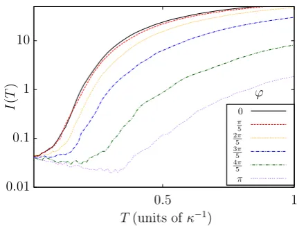
I(T) numerically, we divide the time interval [0, T] into relatively short time intervals ∆t. We then use the quan-tum jump approach [47–49] to simulate a relatively large number of possible quantum trajectories of the cavity and average over the respective number of photon emissions in (T, T + ∆t). The result of this simulation is shown in Figs. 4 and 5. While Fig. 4 shows the average photon emission rateI(T) as a function ofT for different phases

ϕ, Fig. 5 shows theI(T) as a functionϕfor different times

T. Both logarithmic plots illustrate that the dynamics of the mean number of photons inside the resonator de-pends indeed very strongly on the initial coherent state

|αssiof the cavity field.

Next we investigate the accuracy of a measurement, which uses the strong dependence of I(T) on ϕ to de-duce information about ϕ. Figs. 4 and 5 show that this dependence is maximised forϕaround 0.3π. We there-fore consider in the following the signalM =I(T) and

ϕ = 0.3π as an example and calculate the accuracy of the proposed quantum metrology scheme ∆ϕ using the error propagation formula in Eq. (1) as a function of T. The variance in this equation is obtained through statis-tical analysis of the simulation data, while the sensitivity is found by finding the gradient between two very close phases. Again we average over a large number of quan-tum trajectories. The result of this numerical simulation is shown in Fig. 6. To a very good approximation, we find that

∆ϕ(T) ∝ T−0.49 _{for ϕ= 0.3π . (48)}

This means, using only intensity measurements, the ex-perimental setup in Fig. 1 does not allow us to beat the standard quantum limit in Eq. (2). In fact, we almost saturate this limit. This is to be expected as the dy-namics of the mean number of photons inside the cavity

0.01 0.1 1 10

0.5 1

I

(

T

)

T(units ofκ−1)

ϕ

0

π

5 2π

5 3π

5 4π

5 π

FIG. 4: [Color online] Average intensityI(T) plotted on a Log₁₀scale, as a function of the time,T, after the preparation of the initial coherent state,|αssi, for various unknown phases,

ϕ. This simulation assumes|αss|2= 4,η= 0.5 and averages

over 106 _{trajectories.}

0.01 0.1 1 10

0 π

4

π 2

3π

4 π

I

(

T

)

ϕ

T(units ofκ−1₎

0 0.2

0.4

0.6

0.8

1

FIG. 5: [Color online] Average intensityI(T) plotted on a Log₁₀ scale, as a function of the unknown phase,ϕ, for dif-ferent times,T. As in Fig. 4, we have|αss|2= 4,η= 0.5 and

average over 106trajectories.

10−3 10−2 10−1

10−_{2 10}−1 ₁

∆

ϕ

T(units ofκ−1)

FIG. 6: [Color online] Dependence of the accuracy, ∆ϕ, on the length of the measurements stage,T, in the case of intensity measurements. Here, ϕ= 0.3π, |αss|2 = 4, η= 0.5 and we

averaged over 106 _{trajectories. The black line illustrates the}

approximate fit given in Eq. (48).

C. Accuracy of second-order correlation function measurements

A comparison between Figs. 2(a) and (b) suggests that measurements of the joint probability to detect a photon at a timet andat a timet′ _{should be able to reveal} in-formation aboutϕmore efficiently than measurements of the average photon intensityI(T). This joint probability is known to quantum opticians as the second-order pho-ton correlation functionG(2)_{(t, t}′_{). Hence, according to} probability theory,G(2)_{(t, t}′_{) equals}

G(2)(t, t′) ≡ I(t|t′)I(t′), (49)

where I(t|t′_{) denotes the probability for the detection} of a photon at a time t conditional on the detection of a photon at t′_{. Second-order correlation functions are} usually normalised by the product of the photon emission rate att′ _{and att. Taking this into account and dividing} Eq. (49) byI(t′_{)I(t), we define the renormalised} second-order correlation function,g(2)_{(t, t}′_{), by}

g(2)(t, t′_{) ≡} I(t|t′)

I(t) . (50)

This correlation function describes correlations between photon emission events without depending on the detec-tor efficiencyη with which these events are registered. It can therefore be measured accurately, even when using imperfect detectors withη <1.

In the following, we assume thatM =g(2)_{(T,0) is the} actual measurement signal used to obtain information about the unknown phaseϕ. To determine the accuracy ∆ϕof this approach as a function of the lengthT of the measurement stage, we again simulate a relatively large number of quantum trajectories and average over all of

0 1 2 3 4

0 0.5 1 1.5 2

g

(2

) (T

,

0)

T(units ofκ−1)

ϕ

0

π

5 2π

5 3π

5 4π

5 99π

100 π

FIG. 7: [Color online] Second-order correlation function g(2)(T,0), as a function of the duration of the measurement stage,T, for various phases ϕ. Again we assume|αss|2 = 4,

η= 0.5 and averages over 106 _{trajectories.}

0 1 2 3

0 π

2 π

3π

2 2π

g

(2

) (T

,

0)

ϕ

t(units ofκ−1₎

0 0.2

0.5

1 2

FIG. 8: [Color online] Second-order correlation function g(2)(T,0) as a function of the unknown phase, ϕ for vari-ous times,T, with|αss|2 = 4 andη= 0.5 averaged over 106

trajectories.

them. The results of this simulation are shown in Figs. 7 and 8, which are analogous to Figs. 4 and 5 in the pre-vious subsection. As expected, the correlation function

|∂M/∂ϕ|.

This is confirmed by Fig. 9 which shows the depen-dence of ∆ϕon the resource T for phase measurements based on the second-order correlation function for the optimal case of ϕ = π. To calculate this quantity we use again the error propagation formula in Eq. (1) and average over a relatively large number of quantum tra-jectories. We now find that

∆ϕ(T) ∝ T−0.71 _{for ϕ=π (51)}

to a very good approximation. This accuracy clearly beats the standard quantum limit. In other words, mea-surements of the second-order photon correlation func-tion of the photon statistics of an optical cavity inside an instantaneous quantum feedback loop can be very sensi-tive to phase fluctuations.

This is not surprising, since measurements of the second-order photon correlation function g(2)_(T,0) re-quire the detection of single photons. This is different from intensity measurements which are essentially clas-sic measurements. These can be done without high-resolution single-photon detection. Moreover, second-order photon correlations are an intrinsic property of the individual quantum trajectories of the cavity field. They cannot be calculated with the help of a linear master equations but require the quantum jump approach [47– 49], which we introduced in Section III C. The condi-tional dynamics of the individual trajectories of the cav-ity field is in general non-linear. For example, between photon emission, the cavity field evolves in a non-linear fashion with the non-Hermitian conditional Hamiltonian

Hcond in Eq. (35), which requires a constant renormal-isation of the state vector of the quantum system. In summary, it is the measurement of the temporal quan-tum correlations in an open quanquan-tum system that allows us to exceed the standard quantum limit. This observa-tion is consistent with analogous observaobserva-tions by other authors [35–41].

A more standard method of resource counting in quan-tum metrology is to consider the average number of pho-tons that passed through the unknown phase ϕ as the resource N. This approach can also be applied to the quantum-enhanced metrology scheme which we propose here. Performing quantum jump simulations, averaging over many quantum trajectories and using again the er-ror propagation formula in Eq. (1) withM =g(2)_(T,0), we now calculate the dependence of ∆ϕ on the average population of the initial coherent state inside the cavity, which is given by|αss|2. The result is shown in Fig. 10. For the parameters that we consider here, we find that

∆ϕ(|αss|2) ∝

|αss|2

−0.65

for ϕ=π (52)

to a very good approximation. Eq. (52) too clearly beats the standard quantum limit. In practical applications, it might be best to consider both the duration of the mea-surement stage and the number of photons that passed through the sample as a resource. Numerical results for

10−4 10−3 10−2 10−1 1

10−3 ₁₀−2 ₁₀−1 ₁

∆

ϕ

T(units ofκ−1)

FIG. 9: [Color online] Accuracy ∆ϕof the proposed metrol-ogy scheme as a function of the duration of the measurement stage, T, for measurements of the second-order correlation functiong(2)(T,0) aroundϕ=πto maximise the sensitivity of the proposed scheme. As before, we assume |αss|2 = 4,

η = 0.5 and average over 106 trajectories. The black line shows the approximate solution in Eq. (51).

10−5 10−4 10−3

1 10 100

∆

ϕ

|αss|2

FIG. 10: [Color online] Accuracy, ∆ϕ, of the proposed metrol-ogy scheme as a function of the initial mean photon number,

|αss|2, for measurements of the second-order correlation

func-tiong(2)(T,0) andϕ=π. Here,η= 0.5 and we average over 106 _{trajectories. To remove noisy fluctuations in the signal in}

time, we take a sample of uncertainties over a fixed period of time, find the average uncertainty in that period and compare this average to the same time average for other initial states. The black line shows the approximate solution in Eq. (52).

FIG. 11: [Color online] Accuracy ∆ϕplotted on a Log₁₀-Log₁₀ scale, when both the duration of the measurement stage,T, and the initial mean number of photons,|αss|2, is taken into

account and the second-order correlation function g(2)(T,0) is analysed. Here we haveη= 0.5 and we consider 106

repe-titions of the experiment.

V. CONCLUSIONS

This paper proposes a quantum metrology scheme to measure an unknown phase ϕbetween two pathways of light with an accuracy above the standard quantum limit. Our scheme is based on a laser-driven optical cavity in-side an instantaneous quantum feedback loop, as illus-trated in Fig. 1. The measurement process includes two main steps. Firstly, during the preparation stage, a con-tinuous laser experiences the phase shift,ϕ, before enter-ing the cavity field. Its purpose is to prepare the cavity in a coherent stationary state which depends strongly on this phase. Secondly, during the measurement phase, the cavity experiences only the quantum feedback loop. Whenever the spontaneous emission of a photon is de-tected, a laser pulse, which does not experience ϕ and provides the reference frame for the proposed phase mea-surement, is activated and displaces the resonator field in a controlled way.

In this paper we have assumed that the detector that monitors the cavity during the measurement stage de-termines its second-order photon correlation function

g(2)_{(T,0). This means, it essentially measures the joint} probability for the detection of a photon at the very be-ginning (att= 0) and at the end (att=T) of the

mea-surement stage. As shown in Section IV C, this second-order correlation function can be used to determine ϕ

with an accuracy ∆ϕ that scales better than what can be achieved classically according to the standard quan-tum limit in Eq. (2). For the parameters that we con-sider in this paper, we find that ∆ϕ scales as T−0.71 (c.f. Eq. (51)). If we consider instead the mean num-ber of photons seen by the unknown phaseϕduring the preparation stage as the main resource of our quantum metrology scheme, we find that ∆ϕscales as |αss|2

−0.65

(c.f. Eq. (52)).

To achieve this quantum enhancement, our metrology scheme uses the temporal correlations of an individual quantum system instead of using multi-partite entangle-ment. It is worth noticing that subsequent measurements on a single quantum system are in general equivalent to single-shot measurements on multi-partite entangled states. Temporal quantum correlations, which cannot be predicted by a linear master equation, constitute an in-teresting approach for technological applications [37–41]. As shown in Section III, the dynamics of the individual quantum trajectories of the cavity field inside an instan-taneous feedback loop is indeed non-linear and depends very strongly on the initial state of the resonator, which encodes the unknown phaseϕ[29, 30]. As illustrated in Fig. 2, there is constant stretching and growths of the initially occupied phase space volume. The distance be-tween two different states|α1iand|α2iwhich correspond to differentϕ1andϕ2 increases rapidly in time.

The main advantage of the quantum metrology scheme which we propose here is that its experimental realisa-tion is relatively straightforward. As menrealisa-tioned already above, we do not require highly-entangled many-photon states. Although the proposed scheme requires a rela-tively good optical cavity, it does not require highly effi-cient single photon detectors. High-quality optical cavi-ties and relatively fast photon detectors are already avail-able in many laboratories worldwide (see for example Refs. [26–28]). We therefore believe that our quantum metrology scheme will be of significant practical interest until highly-entangled many-photon states become more readily available.

Acknowledgements. We thank C. C. Gerry, P. A. Knott,

B. Maybee, F. Torzewska and G. Vitiello for stimulat-ing and helpful discussions. Moreover, we acknowledge financial support from the UK EPSRC-funded Oxford Quantum Technology Hub for Networked Quantum In-formation Technologies NQIT.

[1] F. Wolfgramm, C. Vitelli, F. A. Beduini, N. Godbout and M. W. Mitchell,Entanglement-enhanced probing of a delicate material system, Nature Photon.7, 28-32 (2013). [2] M. A. Taylor, J. Janousek, V. Daria, J. Knittel, B. Hage, H.-A. Bachor and W. P. Bowen,Biological measurement

[4] J. P. Dowling and K. P. Seshadreesan, Quantum Opti-cal Technologies for Metrology, Sensing, and Imaging, J. Lightwave Technol.33, 2359 (2015).

[5] S. Boixo, A. Datta, S. T. Flammia, A. Shaji, E. Bagan and C. M. Caves,Quantum-limited metrology with prod-uct states, Phys. Rev. A77, 012317 (2008).

[6] V. Giovannetti, S. Lloyd and L. Maccone, Quantum-enhanced measurements: beating the standard quantum limit, Science306, 1330 (2004).

[7] V. Giovannetti, S. Lloyd and L. Maccone, Quantum metrology, Phys. Rev. Lett.96, 010401 (2006).

[8] M. Zwierz, C. A. Perez-Delgado and P. Kok, Ultimate limits to quantum metrology and the meaning of the Heisenberg limit, Phys. Rev. A85, 042112 (2012). [9] B. L. Higgins, D. W. Berry, S. D. Bartlett, H. M.

Wise-man and G. J. Pryde, Entanglement-free Heisenberg-limited phase estimation, Nature450, 393 (2007). [10] C. M. Caves,Quantum-mechanical noise in an

interfer-ometer, Phys. Rev. D23, 1693 (1981).

[11] R. S. Bondurant and J. H. Shapiro, Squeezed states in phase-sensing interferometers, Phys. Rev. D 30, 2548 (1984).

[12] P. Kok, H. Lee and J. P. Dowling,The creation of large photon-number path entanglement conditioned on pho-todetection, Phys. Rev. A65, 052104 (2002).

[13] C. C. Gerry, A. Benmoussa, and R. A. Campos, Non-linear interferometer as a resource for maximally entan-gled photonic states: Application to interferometry, Phys. Rev. A 66, 013804 (2002).

[14] R. A. Campos, C. C. Gerry and A. Benmoussa, Opti-cal interferometry at the Heisenberg limit with twin Fock states and parity measurements, Phys. Rev. A68, 023810 (2003).

[15] S. D. Huver, C. F. Wildfeuer and J. P. Dowling, Entan-gled Fock states for Robust Quantum Optical Metrology, Imaging, and Sensing, Phys. Rev. A78, 063828 (2008). [16] C. C. Gerry, J. Mimih and R. Birrittella,State-projective

scheme for generating pair coherent states in traveling-wave optical fields, Phys. Rev. A84, 023810 (2011). [17] J. Joo, W. J. Munro and T. P. Spiller,Quantum

metrol-ogy with entangled coherent states, Phys. Rev. Lett.107, 083601 (2011).

[18] K. Jiang, C. J. Brignac, Y. Weng, M. B. Kim, H. Lee and J. P. Dowling,Strategies for choosing path-entangled number states for optimal robust quantum-optical metrol-ogy in the presence of loss, Phys. Rev. A 86, 013826 (2012).

[19] P. A. Knott, W. J. Munro and J. A. Dunningham, Attain-ing subclassical metrology in lossy systems with entangled coherent states, Phys. Rev. A89, 053812 (2014). [20] D. W. Berry and H. M. Wiseman, Optimal states and

almost optimal adaptive measurements for quantum in-terferometry, Phys. Rev. Lett.85, 5098 (2000).

[21] C. C. Gerry, Heisenberg-limit interferometry with four-wave mixers operating in a nonlinear regime, Phys. Rev. A61, 043811 (2000).

[22] C. C. Gerry and J. Mimih,The parity operator in quan-tum optical metrology, Contemp. Phys.51, 497 (2010). [23] R. Carranza and C. C. Gerry, Photon-subtracted

two-mode squeezed vacuum states and applications to quan-tum optical interferometry, JOSA B29, 2581 (2012). [24] A. De Pasquale, P. Facchi, G. Florio, V. Giovannetti, K.

Matsuoka and K. Yuasa, Two-Mode Bosonic Quantum Metrology with Number Fluctuations, Phys. Rev. A 92,

042115 (2015).

[25] B. P. Abbott et al. (LIGO Scientific Collaboration and Virgo Collaboration), Observation of Gravitational Waves from a Binary Black Hole Merger, Phys. Rev. Lett.116, 061102 (2016).

[26] A. Kuhn, M. Hennrich, and G. Rempe, Deterministic Single-Photon Source for Distributed Quantum Network-ing, Phys. Rev. Lett.89, 067901 (2002).

[27] J. McKeever, A. Boca, A. D. Boozer, R. Miller, J. R. Buck, A. Kuzmich and H. J. Kimble,Deterministic gen-eration of single photons from one atom trapped in a cav-ity, Science303, 1992 (2004).

[28] E. Pomarico, B. Sanguinetti, P. Sekatski, H. Zbinden and N. Gisin,Experimental amplification of an entangled pho-ton: what if the detection loophole is ignored?, New J. Phys.13, 063031 (2011).

[29] A. V. Masalov, A. A. Putilin and M. V. Vasilyev, Sub-poissonian Light and Photocurrent Shot-noise Suppres-sion in Closed Optoelectronic Loop, J. Mod. Opt. 41, 1941 (1994).

[30] L. A. Clark, B. Maybee, F. Torzewska and A. Beige, in preparation (2016).

[31] H.-P. Breuer and F. Petruccione, The Theory of Open Quantum Systems, Oxford University Press, ISBN: 978-0-19-921390-0.

[32] A. Stokes, A. Kurcz, T. P. Spiller and A. Beige,Extending the validity range of quantum optical master equations, Phys. Rev. A85, 053805 (2012).

[33] H. M. Wiseman and G. J. Milburn,Quantum Measure-ment and Control, Cambridge University Press, ISBN: 978-0-521-80442-4.

[34] L. A. Clark, W. Huang, T. M. Barlow and A. Beige, Hidden Quantum Markov Models and Open Quantum Systems with Instantaneous Feedback in ISCS 2014: In-terdisciplinary Symposium on Complex Systems, Emer-gence, Complexity and Computation14, p. 143, Springer (2015).

[35] D. Braun and J. Martin, Heisenberg-limited sensitvity with decoherence-enhanced measurements, Nat. Com-mun.2, 223 (2011).

[36] K. Macieszczak, M. Guta, I. Lesanovsky and J. P. Garra-han,Dynamical phase transitions as a resource for quan-tum enhanced metrology, Phys. Rev. A93, 022103 (2016). [37] S. Oppel, T. B¨uttner, P. Kok, and J. von Zanthier, Super-resolving multi-photon interferences with indepen-dent light sources, Phys. Rev. Lett.109, 233603 (2012). [38] M. E. Pearce, T. Mehringer, J. von Zanthier and P. Kok,

Precision Estimation of Source Dimensions from Higher-Order Intensity Correlations, Phys. Rev. A 92, 043831 (2015).

[39] M. Guta, Fisher information and asymptotic normal-ity in system identification for quantum Markov chains, Phys. Rev. A,83, 062324, (2011).

[40] D. Burgarth, V. Giovannetti, A. N. Kato and K. Yuasa, Quantum estimation via sequential measurements, New J. Phys.17113055 (2015).

[41] A. H. Kiilerich and K. Mølmer, Bayesian param-eter estimation by continuous homodyne detection, arXiv:1605.00902 (2016).

[42] K. Kraus,States, Effects, and Operations, Lecture Notes in Physics, Volume190, Springer-Verlag (Berlin, Heidel-berg New York, Tokyo, 1983).

[44] C. Emary, N. Lambert and F. Nori, Rep. Prog. Phys.77, 016001 (2014).

[45] A. Stokes, L. A. Clark, and A. Beige, in preparation (2016).

[46] W. H. Zurek,Decoherence, einselection, and the quantum origins of the classical, Rev. Mod. Phys.75, 715 (2003). [47] G. C. Hegerfeldt,How to reset an atom after a photon de-tection: Applications to photon-counting processes, Phys. Rev. A 47, 449 (1993).

[48] J. Dalibard, Y. Castin, and K. Mølmer, Wave-function approach to dissipative processes in quantum optics, Phys. Rev. Lett.68, 580 (1992).

[49] H. Carmichael,An Open Systems Approach to Quantum Optics, Lecture Notes in Physics, Volume 18(Springer, Berlin, 1993).

[50] D. B. Khoroshko and S. A. Kilin, Suppression of pho-tocurrent shot noise in a feedback loop, J. Exp. Theor. Phys.79, 691 (1994).