Towards an improved model of self-interacting dark matter haloes

(1)

Prepared for submission to JCAP

Towards an improved model of

self-interacting dark matter haloes

Anastasia Sokolenko,

1

Kyrylo Bondarenko,

2

Thejs

Brinckmann,

3

Jes´

us Zavala,

4

Mark Vogelsberger,

5

Torsten Bringmann

1

and Alexey Boyarsky

2

1_{Department of Physics, University of Oslo,Box 1048, NO-0371 Oslo, Norway}

2_{Intituut-Lorentz, Leiden University, Niels Bohrweg 2, 2333 CA Leiden, The}

Nether-lands

3_{Institute for Theoretical Particle Physics and Cosmology (TTK), RWTH Aachen}

University, Otto-Blumenthal-Strasse, 52057, Aachen, Germany

4_{Center for Astrophysics and Cosmology, Science Institute,University of Iceland,}

Dun-hagi 5, 107 Reykjavik, Iceland

5_{Department of Physics, Kavli Institute for Astrophysics and Space Research,}

Mas-sachusetts Institute of Technology, Cambridge, MA 02139, USA

E-mail: [email protected], [email protected], [email protected], [email protected], [email protected], [email protected],[email protected]

Abstract.

We discuss the relation between the strength of the self-interaction of dark matter particles and the predicted properties of the inner density distributions of dark matter haloes. We present the results of N-body simulations for 28 galaxy cluster sized haloes performed with the same initial conditions for cold dark matter and for self-interacting dark matter with cross-sections ranging from 0.1 to 10 cm2_/g. We provide a simple phenomenological description of these results and compare them to the semi-analytical model typically used in the literature. We find that some of the assumptions made in this model are not satisfied in the simulations. We identify the reasons for this disagreement and improve the semi-analytical model correspondingly. We discuss how simulation results can be properly compared with observations and in particular how quantities like the core radius and the inner dark matter surface density depend on the self-interaction cross-section.

(2)

1 Introduction

The Cold Dark Matter (CDM) paradigm has been proven to be very successful in describing the large-scale distribution of galaxies and serves as a cornerstone of our current understanding of galaxy formation and evolution (e.g. [1–4]). Self-interacting dark matter (SIDM) [5] is an interesting and well-motivated hypothesis, both from the astrophysics and particle physics perspectives of dark matter (e.g. [6–27] or see [28] for a review). It currently stands as a viable alternative to the CDM paradigm, and as such, the task of constraining the strength of self-interactions from astrophysical observations remains of paramount importance.

(3)

However, we note that the robustness of current constraints on the SIDM cross-section is still debated, in particular due to difficulties in relating observables to quantities that constrain the cross-section (e.g. due to the impact of gas and stars on structure for-mation or due to projection effects) or in properly measuring such observables directly (e.g. the offsets between the dark matter distribution and luminous matter in merging clusters). A lower bound of around 0.1 cm2_/ _{g can be derived from the requirement} that the self-interaction is strong enough for SIDM to be distinct from CDM on small scales (see e.g. [28, 34, 35] for a review), in particular, in order to change the inner structure of dark matter (DM) haloes distinctly from CDM and explain the sizes of DM density cores (e.g. [36–38]), if the latter are robustly confirmed by observations [39]. Apart from systematic errors in observational data and the uncertainties in modeling baryonic effects [39–41], the properties of the haloes and, in particular, the sizes of the cores (if they exist) are expected to have significant scatter, due to individual merger history and specific initial conditions, see e.g. [42] and references therein.

In order to use observational data to determine (or constrain) an intrinsic quantity of DM particles such as its self-interaction cross-section, it is perhaps more efficient to fit the data to the whole ensemble of haloes at the same time. Such a procedure was discussed in [43], where the inner DM surface density, a quantity obeying a well-known scaling law [44, 45] for a halo mass range spanning 6 orders of magnitude, was used to compare SIDM predictions for different cross-sections with observations. The main theoretical uncertainty of this type of analysis is the relation between the observable quantity, the core radius rcore, where the DM density is close to constant ρ(0), and the radiusrSIDM, where self-interactions become important and the velocity dispersion of DM particles is expected to be close to constant. While the former radius, rcore, is more directly connected to observations, the latter,rSIDM, is more directly predicted by theory [26,39,46]. The explicit relation between these two radii for every cross-section has not been discussed in detail in the literature. In order to take into account this theoretical uncertainty, a free phenomenological parameter κ,

κ≡ρ(0)/hρ(rSIDM)i, (1.1) was introduced in Ref. [43]. Here ρ(0) is the central halo density andhρ(rSIDM)iis the average density of the halo within the radiusrSIDM, i.e.hρ(rSIDM)i=M(rSIDM)/ 4₃πr3SIDM

. In this article, we use numerical simulations to remove this uncertainty as far as pos-sible.

(4)

We do not discuss here the effects of baryons on SIDM haloes, as we would like to check the phenomenological description for the DM only case first. For discussion in this direction, see instead [26,47–50], as well as a recent SIDM review [28]. We would like to remark that the model presented in this paper is an improvement over previous models discussed in the literature [39, 47].

This article is organized as follows. We start, in Section 2, by describing the numerical simulations we performed and provide a brief overview of the results, i.e. how SIDM halos differ from their CDM counterparts. In Section 3, we develop an analytic model to describe SIDM halos, which we further refine in Section 4. We then compare predictions of our model to that commonly adopted in the literature, in Section 5, before presenting our conclusions in Section6. In three Appendices we provide further technical details about the simulation results that support the discussion in the main part of the article.

2 Simulations

2.1 Setup

The initial simulation suite used in this work was performed using theAREPOcode [51], with an added module for dark matter self-interactions [19,24]. This simulation suite is described in detail in [37]; in the following we briefly summarize the main aspects relevant for this work. The suite consists of a sample of zoom-in simulations of massive cluster-sized haloes with initial conditions generated with the MUSIC code1 _[₅₂_{] at a}

redshift of z = 50, with an effective resolution of 5123 particles, a softening length of = 5.4kpch−1 _{and particle mass m}

p = 1.271×109 Mh−1. In addition, one halo was

also simulated with a factor of 2 better resolution. The suite presented in [37] consists of 3×28 haloes (and additional 3×1 halo at the higher resolution level) in a CDM and SIDM cosmology, with cross-sections of σ/m = 0.1 and 1 cm2_{/g, starting from} matching initial conditions. For this work, we expand on that suite by re-simulating all 28 haloes with a cross-section of σ/m= 0.5 cm2/g, as well as 10 of those haloes with cross-sections of σ/m= 5 cm2_{/g and}_σ/m_{= 10} _cm2_{/g. Finally we also re-simulated 3} haloes in the sample at the higher resolution level for the CDM and SIDM cosmologies with cross-sections σ/m= 0.1, 0.5 and 1 cm2/g.

All simulations were computed with a cosmology consistent with Planck [53]: with contributions to the energy density of the universe from matter Ωm = 0.315 and cosmological constant ΩΛ = 0.685, dimensionless Hubble parameter h = 0.673, root-mean-square amplitude of perturbations in 8 Mpc h−1 _{spheres today} _σ

8 = 0.83, and tilt of the primordial power spectrum ns = 0.96.

The haloes we study were identified with theSUBFINDalgorithm [54] and are very massive dynamically relaxed2 _{cluster-sized haloes in the mass range M}

200≈0.5−1.9× 1015 _M

h−1 and radius R200 ≈ 1300−2000 kpc h−1, with a peak in the distribution at around M200 ∼ 0.9×1015 M h−1 and R200 ∼ 1550 kpc h−1 (see Fig. A1 of [37]),

1_{https://www-n.oca.eu/ohahn/MUSIC/}

(5)

7.8×1014_M

⊙<M<1.3×1015M⊙

1.3×1015_M

⊙<M<1.7×1015M⊙

0.1 0.5 1 5 10

20 50 100 200

σ/m[cm2/g] rcore

[

kpc

]

7.8×1014_M

⊙<M<1.3×1015M⊙ 1.3×1015_M

⊙<M<1.7×10 15_M

⊙

0.1 0.5 1 5 10

200 300 400 500

σ/m[cm2/g]

Σ

(

rcore

)[

M⊙

/

pc

2 ]

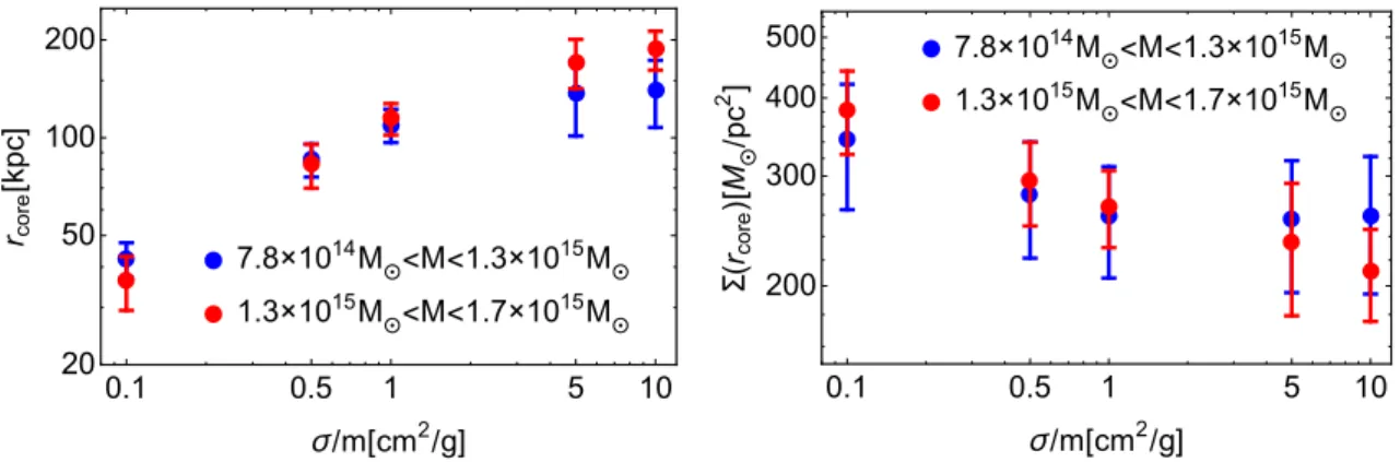
Figure 1: The dependence of rcore (left) and the surface density (right) in SIDM haloes on the self-interaction strength. The data is presented for 2 mass bins with approximately equal scatters of masses. Error bars represent the statistical spread in our suite of simulated haloes and correspond to one standard deviation.

where R200denotes the radius within which the average density is 200 times the critical density of the universe today, ρc = 3H02/(8πG), and M200 the enclosed mass within this radius.

2.2 Properties of SIDM haloes

In a ΛCDM cosmology, DM haloes are expected to have a cuspy density profile that is well described by the universal form suggested by Navarro, Frenk and White (NFW) [56, 57]

ρNFW(r) =

ρs

(r/rs)(1 + (r/rs))2

, (2.1)

where ρs and rs are referred to as the scale density and radius, respectively. An

alternative pair of parameters to describe such profiles is given by the virial massM200 and the halo concentration

c≡ R200 r−2

. (2.2)

where r−2 is the radius where the logarithmic slope of the density profiles equals −2 (i.e. r−2 =rs for the NFW profile). As it turns out, these two parameters

(concentra-tion and mass) are not independent of each other but strongly correlated (which, for example, explains the observed scaling of surface densities [43]). Our simulated CDM haloes follow exactly these general expectations.

If DM is self-interacting, on the other hand, the inner part of a DM halo should develop a core of constant density instead of a cuspy profile, while the outer part of the halo should be unaffected and hence follow the standard NFW profile [5]. We confirm this general expectation in all our simulated SIDM haloes. As shown in the left panel of Fig. 1we also confirm the general expectation that the core radius should grow with the interaction strength. Here and in the following we use the following definition of the core radius rcore:

(6)

The core radius is thus defined as the radius at which the central DM density (from our SIDM simulations or observations) equals the DM density in the CDM case, parame-terized here as NFW profile. The advantage of this definition is that it is in principle observable and independent of the functional form that is used to parameterize the cored profile. A more direct observable quantity that can serve to distinguish between CDM and SIDM haloes is the surface density Σ at this radius [43]. In the right panel of Fig. 1 we show this quantity as a function of the interaction strength. In Fig. 1 we have grouped both rcore(σ/m) and Σ(σ/m) into two mass bins. We see that both quantities saturate around σ/m ∼5 cm2_{/g, the maximal} _r

core being larger for haloes with larger masses.

In the remainder of this article, we will critically assess, and improve, analytical models commonly used in the literature to predict the behaviour shown in Fig. 1 in order to constrain DM self-interactions from observations. While we defer a detailed discussion to later, we can already at this point draw two important conclusions directly from inspection of this figure:

• The core radius shows a relatively weak dependence on the interaction strength. This implies that a small error in estimating the former results in a significant error when deriving constraints on the latter.

• It is fundamentally impossible to constrain cross sections larger than a given limiting value from observations of the core size. For the cluster-sized objects that we have simulated here, this applies to interaction strengths of σ/m _&3 cm2/g. This is because the core has a maximum size set roughly by the radius where the velocity dispersion peaks. Once the core size reaches this value, it becomes insensitive to larger cross sections.

Let us stress that these conclusions are directly based on simulation data, and hence independent of the analytical model that is used to describe self-interactions. In particular, the first point motivates the main goal of this article, which is to obtain a detailed modelling of the effect of DM self-interactions on halo profiles.

3 Analytical model of SIDM haloes

(7)

the Jeans equation relating the 3-dimensional DM velocity dispersion σv(r) and the density profile ρ(r):

d dr

σ_v2 3

r2 ρ

dρ dr

=−4πGr2ρ . (3.1)

In SIDM haloes, the mean-free path λ between collisions is expected to be quite large, much larger than the radius rSIDM:

λ ≡ 1

(σ/m)ρ '4.8 kpc

1 cm2_/g σ/m

1M/pc3

ρ

. (3.2)

This implies that if a kinetic equilibrium can be established within rSIDM, this can only be a global equilibrium, with the same velocity dispersion for all r < rSIDM. Nevertheless, as we see from the simulations, a few collisions per particle in a Hubble time are sufficient to redistribute energy resulting in an isothermal core (constant velocity dispersion) within rSIDM. With this condition, the Jeans equation becomes

¯ σ2_v

3 d dr

r2 ρ

dρ dr

=−4πGr2ρ , (3.3)

where the constant σ¯v describes the average value of the velocity dispersion σv inside rSIDM. This equation has solutions with different asymptotic behaviour at the centre. We anticipate that we do not consider the unphysical solutions where the density goes to zero. We note that the thermalization of the inner core in SIDM haloes is only a quasi-stable configuration. Given enough time, collisions eventually trigger a runaway instability of the core, analogous to the well-known gravothermal catastrophe in globular clusters [60]. The collapse of the core results in a central density profile that is even cuspier than in CDM haloes [61,62]. For this process to be relevant within a Hubble time, however, large cross sections _&10cm2_{/g are required. Our model does} not cover this regime since it is not relevant for the purposes of this work. We will be looking for solutions to the Jeans equation that have a constant density at the center, which is the quasi-stable configuration for relevant cross sections as shown by SIDM simulations in the past. In this model, as we mentioned before, the collision integral is equal to zero on both sides of rSIDM, for different reasons in each regime. In reality, however, there is an intermediate region where the collisions cannot be neglected, but they are still not frequent enough to establish thermodynamical equilibrium. In other words, the model implicitly assumes that the thickness of the intermediate region is much smaller than rSIDM and that it can be approximated by a thin spherical shell at the radiusrSIDM. In this simple, but often adopted model the central regionr < rSIDM is then in thermodynamical equilibrium and the outer region r > rSIDM, where DM particles are effectively collisionless, is connected to the inner region by some boundary conditions at rSIDM. It is clear that in this approximation some quantities will be continuous at rSIDM, but not necessarily all.

(8)

which will be verified below by direct comparison with simulation data. Let us assume that despite self-interactions, DM particles will not leave the radius rSIDM, but will only be redistributed within it. This means that we can choose, as the first boundary condition, the requirement that the mass at rSIDM is the same in the SIDM halo as in the CDM halo:

MSIDM(rSIDM) =MCDM(rSIDM). (3.4)

As for the second boundary condition, we will assume that the kinetic energy defined as

Ekin(r) = 2π

r

Z

0

ρCDM(r)σ2v(r)r

2

dr (3.5)

is equal inside rSIDM for CDM and SIDM

E_kinSIDM(rSIDM) =EkinCDM(rSIDM). (3.6)

These two boundary conditions for the Jeans equation, together with the requirement of a constant density at the centre, allow one to fix the constant velocity dispersion ¯

σv and find a unique solution for the DM density profile. We would like to emphasize that the ansatz where the isothermal profile (3.3) inside the radius rSIDM is connected to a CDM profile at larger radii was already used previously [28,39, 47]. However, as motivated by a direct comparison with our simluation data, we use different boundary conditions compared to earlier works (see also Section 5).

3.1 Verifying the model assumptions with numerical simulations

To verify the validity of the simple model formulated above, we need to explicitly check whether there exists a radius for the simulated haloes inside which, to a certain precision, (i) the masses of CDM and SIDM haloes are equal to each other; (ii) the total kinetic energies of CDM and SIDM haloes are equal; (iii) the velocity dispersions for the SIDM haloes become flat. In this subsection, we will check these assumptions with simulated data for different cross-sections and demonstrate that such a radius exists. In the next subsection, we will check if the Jeans equation (3.3) with our boundary conditions at this radius indeed describes the inner density profile correctly.

We start by definingrM as the radius where, for a given halo, the masses in SIDM

and CDM are equal (see Appendix C for examples of rM for different cross-sections),

and check the hypothesis of equal kinetic energies at this radius. The ratio between kinetic energies in SIDM and CDM simulations is shown in Fig. 2, as a function of the halo concentration as defined in Eq. (2.2). One can see that the kinetic energies of SIDM and CDM profiles inside radius rM agree with an accuracy of .5% for most of

the haloes.

The assumed boundary conditions on equal kinetic energies and masses result in the following average velocity dispersion σ¯v in SIDM haloes:

(¯σpred_v )2 = 2E CDM kin (rM)

MCDM(rM)

(9)

4 5 6 7 0.9

1.0 1.1 1.2 1.3

c

ESIDM

/

ECDM

0.1 cm2_/_g

0.5 cm2/g 1 cm2_/_g

5 cm2/g 10 cm2/g

Figure 2: Ratio of kinetic energies of SIDM haloes to those of the corresponding CDM haloes at the radius of equal massesrM for different values of the self-interaction

cross-section σ/m as a function of halo concentration.

r_M

CDM

σ/m=1 cm2/g

50 100 500 1000

1600 1800 2000 2200

r[kpc] σv

[

km

/

s

]

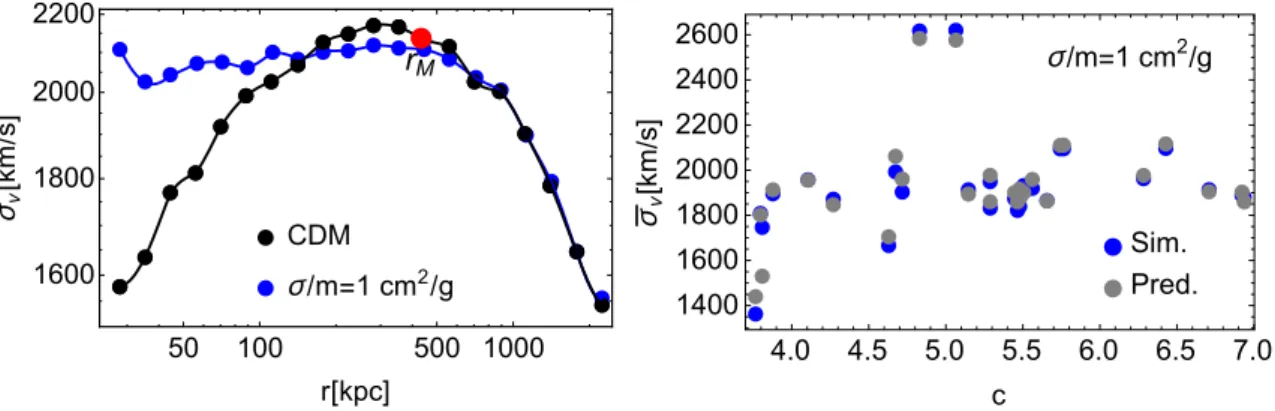
Figure 3: Left panel: Total velocity dispersion profile for an example of a halo in our simulation suite: CDM (black) and SIDM (blue) with σ/m = 1 cm2_{/g. The red} point represents the radius where the enclosed mass is equal in both cases. Right panel: The constant central velocity dispersion σ¯v refers to the average value of the velocity dispersion inside rM (blue) and the predicted value (gray) obtained from the

assumption of equal mass and kinetic energy atrM, see Eq. (3.7). The SIDM case with

σ/m= 1 cm2_{/g is shown as a function of halo concentration.}

The predicted value of the velocity dispersion is compared with the simulation data for σ/m= 1cm2_{/g in the right panel of Fig.}₃_{where we can see that the agreement is} quite good for most haloes. Another assumption we would like to check is the flatness of the velocity dispersion inside rM (see Fig. 3, left panel). Fig.4 shows the deviation

from the best fit constant value of σ¯v, averaged over all radii within rM, for a given

halo as a function of its concentration. We can see that for most of the haloes this deviation is _.1% for σ/m≥1 cm2/g and _.5% for smaller cross-sections.

(10)

Figure 4: The average deviation of the total velocity dispersion in SIDM simulations from the best fit constant value ofσ¯v insiderM for different values of the self-interaction

cross-section σ/m as a function of halo concentration.

rM

Sim.

Pred., isotropic

10 50 100 5001000

5.×10-6

1.×10-5

5.×10-5

1.×10-4

5.×0.00110-4

0.005

r[kpc]

ρ

[

M⊙

/

pc

3 ]

Sim.

Pred., isotropic

3.5 4.0 4.5 5.0 5.5 6.0 6.5 7.0

1 2 5 10 20

c

κ

=

ρ

(

0

)/

<

ρ

(

rM

)>

σ/m=1 cm2/g

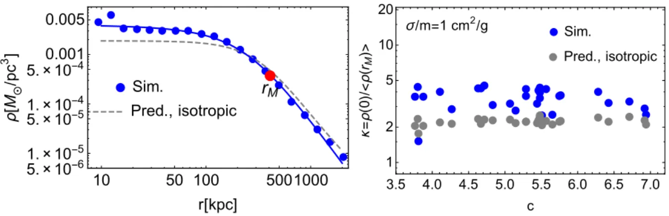
Figure 5: Left panel: Density profiles for a SIDM halo with σ/m = 1 cm2/g from simulations (blue) and the prediction from our isotropic (dashed gray line). Right panel: Ratio between central density and enclosed density at rM for the ensemble of

SIDM haloes with σ/m= 1 cm2/g as a function of halo concentration.

data only as input. This means that we have all elements required to predict the DM density profile as a solution of the Jeans equation with constant velocity dispersion σ¯v. This prediction will provide a validity check of our model.

3.2 Verifying the model prediction for the density profile

(11)

4 5 6 7 0

1 2 3 4 5 6

c

κsim

/

κpred

iso

0.1 cm2/g

0.5 cm2/g

1 cm2_/_g

5 cm2/g

10 cm2/g

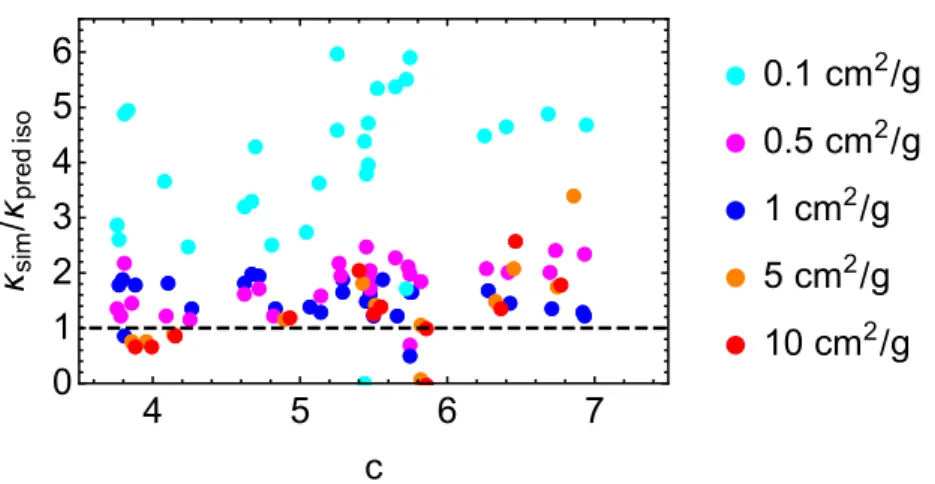
Figure 6: The ratio of κ=ρ(0)/hρ(rM)i between simulated and predicted values for

our isotropic model versus halo concentration in SIDM haloes for different values of the self-interaction cross-section σ/m.

CDM 0.1 cm2_/g

1 cm2_/g

5 cm2_/g

50 100 500 1000

-0.4 -0.2 0.0 0.2 0.4

r[kpc]

β CDM

0.1 cm2_/g

1 cm2_/g

5 cm2_/g

50 100 500 1000

-0.4 -0.2 0.0 0.2 0.4

r[kpc]

β

Figure 7: Velocity anisotropy profiles β(r) = 1−(σ2

θ +σφ2)/(2σr2) from simulations

for CDM (black) and SIDM (cyan, blue and orange for σ/m = 0.1, 1 and 5 cm2/g, respectively) for two different example haloes. The vertical green line marks the rM

radius.

haloes.

3.3 Anisotropy of the velocity dispersion

A perfect equilibrium would imply that all components of the velocity dispersion are isotropic. Therefore the anisotropy of the velocity dispersion

β(r) = 1− σ

2

θ +σφ2

2σ2

r

(3.8)

should be equal to zero, where σθ,φ are the velocity dispersions in the tangential

direc-tions, whileσris the radial velocity dispersion. However, in the simulations, we observe

that the anisotropyβ for SIDM haloes does not vanish inside the radius rM, where full

(12)

Best fit values ofβ =Aln(r/rβ)

σ/m[cm2_/g_] _A _r

β[kpc]

CDM 0.067 13.7

0.1 0.074 21.8

0.5 0.089 50.1

1 0.102 76.4

5 0.124 194

10 0.166 387

Table 1: The best fit values for the anisotropy profile β(r) (Eq. 3.9) from simulated haloes in CDM and SIDM for different cross sections.

50 100 500 1000

0.0 0.1 0.2 0.3 0.4 0.5

r[kpc]

β

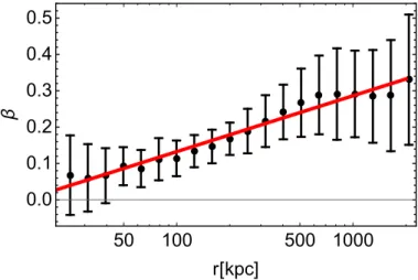
Figure 8: Velocity anisotropy versus radius for the CDM haloes. Black dots are mean values for the given radius bin and error bars represent the standard deviation. The red line is the best fit with ansatz (3.9) (see Table 1 for values of the fit parameters).

comparable to that of CDM haloes and does not drop to zero fast enough inside rM to

be neglected, which means that thermal equilibrium is not fully established; at least not for σ/m_.1 cm2/g.

The velocity anisotropy of DM particles is of course not directly observable. To make our model less dependent on simulation input, we would like to come up with a prescription which can be applied not only to simulated data, where we know all quantities but to observational data in the future. We have found that a simple two-parametric ansatz

β(r) =

Aln(r/rβ), for r≥rβ

0, for r < rβ

(3.9)

describes β(r) for a given cross-section reasonably well, for both the SIDM and CDM cases. The best fit values of the parametersA andrβ are presented in Table1, see also

(13)

rM Sim.

Pred., isotropic

Pred.(<β>), anisotropic

10 50 100 5001000

5.×10-6

1.×10-5

5.×10-5

1.×10-4

5.×0.00110-4

0.005

r[kpc]

ρ

[

M⊙

/

pc

3 ]

Sim.

Pred., isotropic

Pred.(<β>), anisotropic

3.5 4.0 4.5 5.0 5.5 6.0 6.5 7.0

2 5 10 20

c

κ

=

ρ

(

0

)/

<

ρ

(

rM

)>

σ/m=1 cm2/g

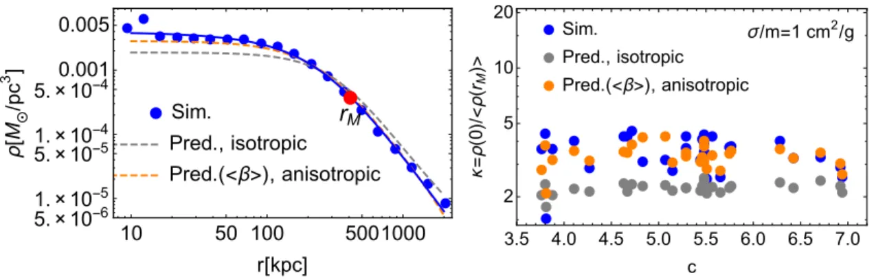
Figure 9: Left panel: Density profiles versus radius for a SIDM halo with σ/m = 1 cm2_{/g from simulations (blue) and the prediction for the SIDM profile from our} isotropic (dashed gray line) and anisotropic models (orange line). The red dot indicates therM radius. Right panel: κ=ρ(0)/hρ(rM)ias a function of halo concentration

calcu-lated from the simulation data forσ/m= 1cm2_{/g (blue), and our isotropic/anisotropic} model (gray/orange).

We will use the above ansatz forβ(r)to improve our model and predict the density for SIDM using the anisotropic Jeans equation in the following.

3.4 Prediction for the density profile with anisotropic Jeans equation

Although there is no equilibrium inside rM, we can still use the Jeans equation if we

take into account the velocity anisotropy β(r). The anisotropic Jeans equation for the radial velocity dispersion σr is [63]

d dr

r2 ρ

d dr ρσ

2

r

+ 2rβσ2_r

=−4πGr2ρ , (3.10)

where the radial velocity dispersion σr is connected to the total velocity dispersion σv as

σ_v2 ≡σ_r2+σ2_θ+σ_φ2 =σ2_r(3−2β). (3.11) In Eq. 3.10 we can still use the assumption that the total velocity dispersion is a constant as this is consistent with the simulated data. With the addition of velocity anisotropy into the Jeans equation, we significantly improve the accuracy of our model (see Fig. 9). Moreover, the predictions for the SIDM density profiles using our ansatz forβ(r)now becomes very similar to using the actual velocity anisotropy directly from each simulated halo.

As demonstrated in Fig.10, the prediction for the density profile with the anisotropic Jeans equation for the other SIDM cross sections is also consistent with the simulated data. This indicates a good agreement between the anisotropic modelling and the simulations. We note, however, that the modelling is less accurate at smaller cross sec-tions, particularly for σ/m∼0.1 cm2_{/g, where the central SIDM halo is farther from} equilibrium. This is reflected in the dependence of the parameter κ = ρ(0)/hρ(rM)i

(14)

4 5 6 7 0

1 2 3 4

c

κsim

/

κpred

aniso

0.1 cm2_/_g 0.5 cm2_/_g 1 cm2_/_g 5 cm2_/_g 10 cm2_/_g

0.1 0.5 1 5 10

0 2 4 6 8

σ/m[cm2_/_g_]

κsim

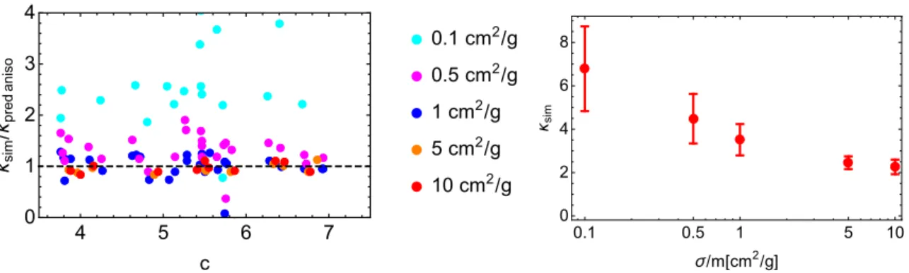
Figure 10: Left panel: The ratio of the simulated κ values in SIDM haloes to the predicted ones for our anisotropic model for different values of the self-interaction cross-section σ/m as a function of halo concentration. Right panel: The value κsim = ρ(0)/hρ(rM)iin our SIDM haloes for different values of the self-interaction cross-section

σ/m. The central point is the meanκsim value for a given cross-section in simulations, while error bars correspond to one standard deviation.

3.5 Connecting our model to the CDM NFW parameters

Now we can try to emulate an actual data analysis with a more realistic approach. At large radii, SIDM profiles are well fitted by NFW profiles and, in this region, we usually have the best observational data. Therefore, we would like to only use the NFW profile to predict the SIDM density profiles for a given cross-section. The only input we will then need from simulations is the radius rSIDM, which we showed above to be well represented by the radius of equal masses rM. Predicting rM for every

asymptotic NFW profile and each value of the cross-section is a non-trivial task and we leave it for the next section.

The method described and tested above also requires the velocity dispersion profile for the corresponding CDM halo as input. We can obtain it by using the NFW profile and solve the anisotropic Jeans equation (see Appendix B) with the anisotropy β(r) described by the ansatz (3.9) (the same for each CDM halo, similarly to what we did for SIDM), see Table 1. As a result of this procedure, we can obtain the velocity dispersion profile for a given CDM halo (for an example, see the left panel of Fig. 11). Using the CDM velocity dispersion profile for a given halo, we predict the constant value for the corresponding central SIDM velocity dispersion σSIDM

v , see right panel of Fig. 11.

(15)

CDM Pred.

50 100 500 1000

1400 1500 1600 1700 1800 1900 2000

r[kpc]

σv

[

km

/

s

]

Figure 11: Left panel: Total velocity dispersion profile for an example of a simulated CDM halo (black points) and the predictions based on the NFW density profile and the anisotropic Jeans equation (blue line). Right panel: Central total velocity dispersion ¯

σv inside rM as a function of concentration in simulated SIDM haloes (blue), and

predicted values (gray) for the case σ/m= 1cm2_{/g. To make this prediction, we have} used the NFW parameters of the corresponding CDM halo; see text for details.

4 5 6 7

0 1 2 3 4

c

κsim

/

κpred

NFW

0.1 cm2_/g 0.5 cm2_/g

1 cm2_/g 5 cm2_/g 10 cm2_/g

4.0 4.5 5.0 5.5 6.0 6.5 7.0 0

1 2 3 4 5

c

κ

σ/m=1 cm2_/_g

Sim. From SIDM From NFW

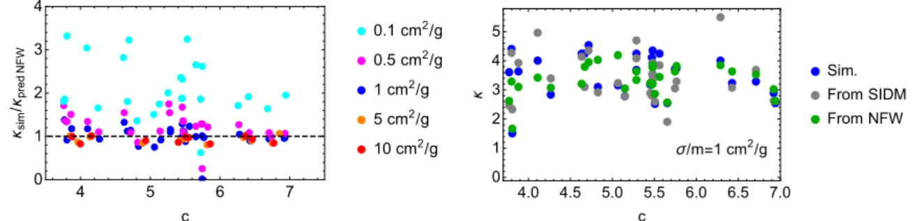
Figure 12: Left panel: The ratio between simulated and predicted values of κ in SIDM haloes as a function of halo concentration for our anisotropic model using as input only the NFW parameters of the corresponding CDM haloes. Right panel: Den-sity ratios κ versus halo concentrations, for σ/m = 1 cm2_{/g, taken directly from our} simulations (blue), from our anisotropic model using data from the SIDM simulations (gray), and with our full model using only the NFW parameters of the corresponding CDM simulations as input (green).

(16)

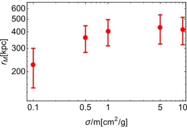
0.1 0.5 1 5 10 200

300 400 500 600

σ/m[cm2/g]

rM

[

kpc

]

Figure 13: The dependence ofrM on the cross-section. The error bars represent the

standard deviation of the distribution.

4 From the cross section to the radius

r

M

Ideally, we would like to directly connect the observationally accessible core radius defined in Eq. (2.3), see also Fig. 1, to the predictions from our SIDM model. In the previous sections, we have checked that the radiusrSIDM, where equilibrium is assumed to be established, could be chosen as the radiusrM, where the enclosed mass and kinetic

energy in SIDM haloes are the same as in their CDM counterparts. The dependence of rM on cross-section is shown in Fig. 13. Using this radius, one is able to predict,

with sufficient accuracy (see the discussion in the previous section), the density profile for a SIDM halo using the data for a CDM halo with the same initial conditions. This means that we can relate the "observed" core radius torSIDM. To complete the picture, we now need to connect rSIDM with the self-interaction cross section σ/m.

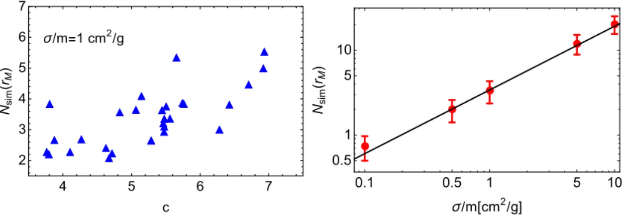
In the literature (see e.g. [28, 39]), the relation between these quantities is often defined by the requirement of having at least one collision per particle inside rSIDM, over the halo age tage. We would like to check to what extent this condition is satisfied in simulations, so we show in Fig. 14 the average number of collisions per particle at radius rM. This clearly demonstrates that Nsim.(rM) varies significantly in our

simulation suite. We also find thatNsim(rM)does not scale exactly linearly withσ/m,

instead we find the best-fit slope of the power law to be 0.75(right panel of Fig. 14). In Refs. [28, 39] the number of collision per particles at radiusr is estimated as

Nl(r)≡ σ

mρ(r)v(r)tage, (4.1)

where v(r)is the average relative velocity of DM particles at radius r andtage we take as half-mass formation time, see Ref. [43] for details. The condition of one collision per particle per halo age thus translates to the often quoted

σ

mρ(rSIDM)v(rSIDM)tage = 1. (4.2)

Substituting v(r) = (4/√3π)σ_vSIDM(r), we have compared the values of Nl(rM)

(17)

▲ ▲ ▲ ▲ ▲ ▲ ▲▲ ▲ ▲ ▲ ▲ ▲ ▲ ▲ ▲ ▲ ▲ ▲ ▲ ▲ ▲ ▲ ▲ ▲ ▲ ▲ ▲ ▲ ▲ ▲ ▲ ▲ ▲ ▲▲ _▲_▲ ▲ ▲ ▲ ▲ ▲ ▲ ▲ ▲ ▲ ▲ ▲ ▲ _▲_▲ _▲_▲ ▲ ▲ ▲ ▲

4 5 6 7

2 3 4 5 6 7 c Nsim ( rM )

σ/m=1 cm2/g

0.1 0.5 1 5 10

0.5 1 5 10

σ/m[cm2/g]

Nsim

(

rM

)

Figure 14: Left panel: The average number of collisions at radiusrM as a function of

halo concentration for σ/m= 1 cm2_/g. _{Right panel:} _{The average number of collisions} at radius rM for different cross-sections. The black line shows the best fit power law

dependence, N(rM)∝(σ/m)0.75.

cross-sections 5 cm2_{/g and} ₁₀_cm2_{/g (the latter is shown in the top right panel of} Fig. 15), but the predictions from Eq. (4.1) are systematically lower for smaller cross-sections (see top left panel of Fig.15for the case withσ/m= 1 cm2/g). In the bottom panel of Fig. 15we furthermore show typical examples of the radial dependence of the number of collisions, N(r), found in the simulations. Clearly, Eq. (4.1) provides an incorrect prediction of this dependence.

Following Ref. [43] we have also checked a modified Eq. (4.2) for the number of collisions per particle inside rSIDM,

σ

mhρ(rSIDM)iv(rSIDM)tage = 1, (4.3) wherehρ(rSIDM)i= 3M(rSIDM)/(4πrSIDM3 )is the average density of the core. In analogy to Eq. (4.1), we thus have

N(r)≡ σ

mhρ(r)iv(r)tage, (4.4) We repeated the same analysis for the average number of collision inside the radiusrM,

hN(< rM)i, and found results similar to the previous case, see Fig. 16. We conclude

that neither Eq. (4.1) nor Eq. (4.4) can be reliably used to connect rSIDM with σ/m. Below, we discuss a simple toy model that improves upon this situation by qualitatively explaining the behaviour of N(r)at large radii.

4.1 Radial infall model for how the number of collisions depends on the radius

Let us for simplicity consider the case of a stationary halo in which the DM particles are only moving on radial orbits. The orbit period T, with maximal radius rmax, is then determined by the gravitational field as

T(rmax) = 2

Z rmax

0

dr

(18)

▲ ▲ ▲ ▲ ▲ ▲ ▲▲ ▲ ▲ ▲ ▲ ▲ ▲ ▲ ▲ ▲ ▲ ▲ ▲ ▲ ▲ ▲ ▲ ▲ ▲ ▲ ▲ ▲ ▲ ▲ ▲ ▲ ▲ ▲▲ _▲_▲ ▲ ▲ ▲ ▲ ▲ ▲ ▲ ▲ ▲ ▲ ▲ ▲ _▲_▲ _▲_▲ ▲ ▲ ▲ ▲

4 5 6 7

0 1 2 3 4 5 6 7 c N ( rM )

σ/m=1 cm2/g

▲ ▲ ▲ ▲ ▲ ▲ ▲ ▲ ▲▲ ▲▲ ▲ ▲ ▲_{▲ ▲▲} ▲ ▲ ▲ ▲

4 5 6 7

0 10 20 30 40 50 60 c N ( rM )

σ/m=10 cm2/g

▲▲ ▲ ▲ ▲ ▲ ▲ ▲ ▲ ▲ ▲ ▲ ▲ _{▲ ▲} ▲ ▲ ▲ ▲ ▲

10 50 100 500 1000

0.5 1 5 10 50 100

r[kpc]

N

(

r

)

σ/m=1 cm2/g

▲

▲ ▲▲ ▲ ▲ ▲ ▲ ▲ ▲ ▲ ▲ ▲ ▲ ▲ _{▲ ▲}

▲_▲

▲

10 50 100 500 1000

0.5 1 5 10 50 100

r[kpc]

N

(

r

)

σ/m=10 cm2/g

Figure 15: The average number of collisionsinsideradiusrM (dots) and atradiusrM

(triangles) versus halo concentration for σ/m= 1cm2_{/g (top left) and}₁₀ _cm2_{/g (top} right). The lower panels show example halos with σ/m= 1 cm2_{/g (lower left) and} ₁₀ cm2/g (lower right) where we plot, as a function of radius r, the number of collisions inside (dots) and at r (triangles). Blue and red points are the simulation data, while the grey dots (upper panels) and grey lines (lower panels) are the predictions from Eq. (4.1). The green dashed line in the lower panels marks the radiusrM.

where the velocity v(r)follows from energy conservation as

U(rmax) =U(r) + v2₍_r₎

2 with U(r) =

Z r

0

GM(r)

r2 dr . (4.6)

During the halo age tage, a particle travels through the center of a halo tage/T times. The average number of scatterings per center crossing is

NT(rmax) = 2

Z rmax

0 σ

mρ(r)dr , (4.7)

where we neglected the change of the particle trajectory after scattering. Therefore, the total number of collisions for this particle during its lifetime is

Nmax(rmax) = tage T(rmax)

(19)

4 5 6 7 2

3 4 5 6 7

c

〈

Nsim

(<

rM

)

〉

σ/m=1 cm2/g

0.1 0.5 1 5 10

1 5 10

σ/m[cm2/g]

〈

Nsim

(<

rM

)

〉

Figure 16: Left panel: Average number of collisions inside radius rM as a function

of halo concentration for σ/m = 1 cm2_/g. _{Right panel:} _{Average number of collisions} inside rM for different cross-sections. The black line shows the best fit power-law

dependence, hN(< rM)i ∝(σ/m)0.63.

Eq. (4.8) gives the number of collisions for a particle with the maximal radius rmax, while from the simulations we can extract the average number of collisions per particle for particles that are found at a given radius r atz = 0. To connect these two numbers we determine the maximal radius of a particle with a given velocityrmax(r, v), using (4.6), and then average over the velocity distribution of the DM particles f(r, v) at radius r,

N(r) =

Z

Nmax(rmax(r, v))f(r, v)dv . (4.9)

This formula reduces to Eq. (4.1) in the case v(r) =const, ρ(r) =const.

Since the velocity distribution f(r, v) is not known a priory in our modelling, however, we are in general forced to use the radial velocity dispersion σr instead of

averaging as in Eq. (4.9). This introduces an uncertainty which can be parameterized by an unknown factor C of order one:

Nour(r) = CNmax(rmax(r, σr)). (4.10)

In Fig. 17 we show an example of how well this ansatz works for C = 2.5 and σ/m= 1 cm2_{/g. We generally find that the ansatz (}_4.10_{) provides a good description for the} average number of collisions inside a given radius hNsim.(< r)i (left panel), while it works not so well for the number of collisions ata given radius Nsim.(r) (right panel). Although the qualitative behaviour of the simulations is well described by this simple ansatz, it is clear that it requires improvement for a fully quantitative description.

4.2 Phenomenological modelling for the radial profile of the number of collisions

(20)

50 100 500 1000 2

4 6 8 10

r[kpc]

N

(

r

)

σ/m=1 cm2/g

▲ ▲ ▲ ▲ _{▲ ▲} ▲

▲ ▲

50 100 500 1000

2 4 6 8 10

r[kpc]

N

(

r

)

σ/m=1 cm2/g

Figure 17: The average number of collisions per particle inside (left) and at (right) radius rforσ/m= 1 cm2/g (blue points). The red line is the prediction from a simple radial infall model, see Eq. (4.10).

10 50 100 500 1000

2 4 6 8 10

r[kpc]

〈

Nsim

(<

r

)

〉

σ/m=1 cm2/g

0.1 0.5 1 5 10

100 200 500

σ/m[cm2/g]

rN

[

kpc

]

Figure 18: Left panel: Illustration of how we have defined the radiusrN (black dashed

line) for the number of collisions profile N(r), as the radius where the asymptotic behaviour (modeled as power laws) of the small and large radii cross each other (black solid lines). The blue points are the average number of collisions inside a given radius for σ/m = 1 cm2_/g. _{Right panel:} _{The dependence of the radius} _r

N on the

cross-section for our simulated suite. The error bars represent the standard deviation of the distribution.

at the simulation results, we observe that the radial dependence on N(r) is very flat, hence, conditions of the typeN(rM) = constwould always produce a large uncertainty

on the estimated value of rM. However, N(r) seems to have a characteristic radius

rN, where the slope of the profile changes substantially. This scale can be defined,

for example, as the radius where the power laws of the asymptotic behaviour at small and large radii cross each other. An illustration of this definition of rN is shown in

the left panel of Fig. 18, where we used the average number of collisions inside a given radius hNsim.(< r)i as a proxy for N(r) in simulations. The scaling of rN with the

(21)

0.1 0.5 1 5 10 0.50

0.75 1.00 1.25 1.50

σ/m[cm2/g]

rN

/

rM

Figure 19: The cross-section dependence of the ratio of the two radii rN (connected

to the radial dependence of the average number of collisions) and rM (defined as the

radius within which the mass and kinetic energy are the same as in for CDM). The error bars represent the standard deviation of the distribution.

coincide. The necessary conditions for a single scaling radiusrSIDMin our SIDM model, which we discussed in Section3.1, are satisfied more poorly atrN than they are atrM,

hence, we cannot replace rM by rN. Moreover, the ratio between rN and rM depends

on the cross-section (see Fig. 19). In turn, the dependence of rM on the cross-section

is rather weak (see Fig. 13) and it cannot be used to define σ/m with confidence: a small error in estimating rM results in a large uncertainty for the estimated σ/m.

We conclude that, although we are able to construct an improved model that can relate the radius rSIDM in SIDM haloes to observables (the inner density profile and, in particular, the core radius), we can still not robustly relate this radius (and hence a potential observable) to the self-interaction cross-section σ/m. This limitation is caused by a complex dependence of the properties of simulated SIDM haloes on the value of the cross-section, which conflicts with the simple estimate used in previous analytical models in the literature, based on a constant average number of collisions per particle and halo time in the SIDM halo core.

5 Comparison with previous approaches

Let us finally compare predictions from our method with those based on the method commonly adopted in the literature [28], with a focus on observationally accessible quantities like the core radius. As a reminder of our discussion in Section 3, the Jeans equation requires two boundary conditions (and has one free parameterσ¯v), which we choose as ρ0(0) = 0 (cored solution) and MCDM(rSIDM) = MSIDM(rSIDM). This still leaves the determination of the transition scale rSIDM. In the method used in this work both predicted ρSIDM(0) and σ¯v agree with simulations (see e.g. Figs. 3and 10).

(22)

Our prediction

“1 col./par.”, method A Data

0.1 0.5 1 5 10

50 100 500 1000

σ/m[cm2/g]

rcore

[

kpc

]

Figure 20: We compare the core radius (2.3) from simulation data (red), our predic-tions from this work (blue) and the predicpredic-tions obtained by following what we describe as method A in the text (green), using an isotropic Jeans equation and imposing the equal mass boundary condition at the “one collision per particle” radius.

0.1 0.5 1 5 10 1.0

1.1 1.2 1.3 1.4

σ/m[cm2/g]

ρSIDM

(

rSIDM

)/

ρCDM

(

rSIDM

)

Figure 21: Density ratios of simulated SIDM and CDM halos, at radiusrSIDM, versus cross-section.

particle” and halo time, cf. Eq. (4.2). To fix the density profile we also need to knowσ¯v, which we take directly from the SIDM simulations. We call this approach method A. In Fig. 20, we compare simulated core radii with those predicted by the two methods. Here, we choose our standard definition of the core radius, Eq. (2.3), but stress that the qualitative features of this figure would not change with alternative definitions. Clearly, the predictions frommethod Aare not consistent with the simulation data. Our method, on the other hand, is in excellent agreement with the data forσ/mχ&1cm2/g;

for smaller cross sections, it slightly overpredicts the expected core size.

(23)

“1 col./par.”, method B

0.1 0.5 1 5 10

0.0 0.5 1.0 1.5 2.0 2.5 3.0

σ/m[cm2/g] rcore

1

col

/

rcore

“1 col./par.”, method B Sim.

0.1 0.5 1 5 10

1250 1500 1750 2000 2250 2500

σ/m[cm2_/_g_] σv

,

c

[

km

/

s

]

Figure 22: Left panel: Ratio between core radii of SIDM halos predicted from CDM halo profiles using the commonly adopted method in the literature (method B) and core radii in SIDM simulations versus cross-section. Right panel: Average velocity dispersion inside rSIDM for simulation data (red) and predictions (cyan) formethod B.

defined by the “one collision per particle” condition). We call this approach method B. Let us remark that the condition of a continuous density profile must be satisfiediffthe transition zone between the region of equilibrium (which is well described by the Jeans equation) and the outer region (described by a standard CDM halo) is infinitely thin. In reality, one would expect a more extended transition region where self-interactions neither fully thermalize the halo nor leave it completely unaffected. Around the point rSIDM where the boundary is formally placed, both the solution of the Jeans equa-tion and the outer (typically NFW) profile are then only extrapolaequa-tions that do not describe the actual density profile; hence, it is not obvious why these profiles should match exactly at r = rSIDM). An explicit comparison with simulations, as shown in Fig. 21, reveals that this is indeed not the case. In the left panel of Fig. 22, we plot the ratio of the core radius obtained with method B to that found in our simulations. As pointed out previously, e.g. Refs. [20, 30, 39], this leads to very good agreement. However, as demonstrated in the right panel of Fig.22, the predictions for the velocity dispersion σ¯v are clearly not compatible with the simulation results. In view of the failures to correctly reproduce both σ¯v and the density ratio at the transition point, we are thus lead to conclude that the success of method B in predicting the core radii is at least partially based on a numerical coincidence.

(24)

6 Summary and conclusion

In order to constrain the SIDM cross-section from observed dynamical properties of galaxies or clusters of galaxies, one can adopt either of the following two methods:

• Use a large number of numerical simulations and a careful mapping between direct observables and simulated quantities. This approach captures the relevant physical processes and gives a full prediction for the structure of SIDM haloes.

• Use an analytical model that accurately captures the effect of dark matter self-scattering on observables. This approach has the advantage of requiring much less computational time, while being able to compare models to data for a wide range of halo masses, but requires a physically motivated model with several assumptions, which are tuned and tested against simulations.

In this paper, we have taken a revised look at the second approach, with the goal of improving the analytical modelling of SIDM haloes. A summary of our main findings is as follows:

• The models currently used in the literature do not explain the simulation results in a satisfactory manner. In particular the basic underlying formula (4.2) for one collision per particle and halo age is not supported by simulations, see Figures14 and15. Also, we found that the velocity anisotropy is not zero (see Fig.7), which significantly changes the predictions for the density profiles (see Figures 9, 10).

• We have introduced an improved model, which takes as input the large radii behaviour of SIDM haloes that asymptotically reaches the CDM predictions (parameterized with the NFW profile), and matches it to the solution of the anisotropic Jeans equation with a constant velocity dispersion at a radius rSIDM (see Fig.20for the comparison of our analytical results with the data and analyt-ical predictions made by the isotropic Jeans equation with equal mass boundary conditions at “one collision per particle radius”), see Section 5 for details. For a given halo with fixed NFW parameters, our model gives a good prediction of the properties of the corresponding SIDM halo (core size and density) as a function of the cross section if the radius rSIDM is taken from the simulated halo. The boundary condition imposed to define rSIDM in our model is to match the mass of the CDM and SIDM haloes within rSIDM. A second boundary condition, im-posing the same kinetic energy withinrSIDM, fixes the central velocity dispersion, which finally closes the system allowing us to find a unique SIDM profile.

(25)

• Our model improves upon isotropic models by allowing for a radially-dependent velocity anisotropy β(r), taking into account that the SIDM simulations show a non-zero anisotropy within rSIDM for σ/m <5 cm2/g. Indeed, β could be up to 0.2 in the region of interest. This demonstrates that equilibrium is not fully established inside rSIDM, even if the total velocity dispersion is quite close to constant. We have taken this effect into account by using a simple ansatz for the velocity anisotropy, which is the same for all haloes (but with parameters that depend on the cross-section and are fitted to the simulations; see Table 1).

Our model would be complete if, for each halo and for a given cross-section, we could predict rSIDM. This has been done by fixing the (radially-dependent) number of collisions per particle N(r), as N(rSIDM) = 1. We have found, however, that we could not complete our model, in this sense, for the following reasons:

• In the simulations, N(rSIDM) is not equal to 1, but instead depends on the con-centration of the halo and on the cross-section. N(r) in simulated haloes is a slowly-varying monotonic function of radius, flattening at the center. Because of this, a condition like N(rSIDM) ∼ 3−5 would fix rSIDM with an uncertainty of up to an order of magnitude. Therefore, even if we were able to measure rSIDM from observations, this would not help us to fix the cross-section, σ/m, as the uncertainty in the relation betweenrSIDMandσ/mviaN(r) = const.is too large.

• We have tried to model the radial dependence of the number of collisions by defining a scale radius rN where the slope of N(r) changes most abruptly,

ef-fectively separating a central flat behaviour from an outer power law. Although this radius correlates strongly with the cross-section, the ratio of rN and rSIDM also changes with the cross-section. Because of this, although we built a simple model that roughly explains the radial dependence ofN(r), we ultimately cannot relate σ/m to observables (e.g the core size) in an accurate way.

• This limitation seems to be fundamentally driven i)on the low-end of the cross-sections studied here by the lack of full thermalization of the core (up to the maximum size it can take), and ii) at the high-end of the cross sections due to the saturation of the core and the triggering of an on-setting gravothermal collapse. Therefore, the range of cross sections where an equilibrium model can in principle be used, even with our suggested improvements, is indeed quite narrow.

(26)

Acknowledgements

(27)

50 100 500 1000 -0.2

0.0 0.2 0.4 0.6

r[kpc]

β

CDM

50 100 500 1000

-0.2

0.0 0.2 0.4 0.6

r[kpc]

β

σ/m=0.1 cm2/g

10 50 100 500 1000

-0.2

0.0 0.2 0.4 0.6

r[kpc]

β

σ/m=0.5 cm2/g

50 100 500 1000

-0.2

0.0 0.2 0.4 0.6

r[kpc]

β

σ/m=1 cm2/g

10 50 100 500 1000

-0.2

0.0 0.2 0.4 0.6

r[kpc]

β

σ/m=5 cm2/g

10 50 100 500 1000

-0.2

0.0 0.2 0.4 0.6

r[kpc]

β

σ/m=10 cm2/g

Figure 23: Velocity anisotropy profiles for all haloes in our simulations (gray lines), for CDM and SIDM with cross-sectionsσ/m= 0.1cm2_/g,₀_.₅_cm2_/g,₁_cm2_/g,₅_cm2_/g and 10 cm2_{/g. The red line is given by the ansatz (}_3.9_{) with the best-fit parameters} stated in Table 1.

A

Radial velocity anisotropy profile

β

(

r

)

We have adopted a simple two-parameter ansatz to fit the mean behaviour of the ve-locity anisotropy profile in the ensemble of our simulated haloes:

β(r) =

Aln(r/rβ), for r≥rβ

0, for r < rβ

(A.1)

(28)

In Fig. 23we show the result of this procedure along with the data (the best fit values of the parameters A and rβ are presented in Table1).

B

From the NFW parameters of the CDM halo to the model

of the SIDM halo

The density, radial velocity dispersion, and velocity anisotropy profiles of collisionless CDM haloes are connected through the Jeans equation:

d dr σ

2

r(r)ρ(r)

+2 rβ(r)σ

2

r(r)ρ(r) =−ρ(r)

GM(r)

r2 (B.1)

Therefore, one can find the velocity dispersion profile in CDM haloes using as input the profiles for density and velocity anisotropy. To show this, we introduce the function f(r) = σ2

r(r)ρ(r)to write Eq. B.1:

df dr +

2

rβ(r)f(r) =−ρDM(r)

GMDM(r)

r2 , (B.2)

and we use the method of variation of constants to solve this equation. The solution of the homogeneous equation

df dr +

2

rβ(r)f(r) = 0 (B.3)

is

f(r) =C1e

−2Rr

r0

β(y)

y dy _. _(B.4)

We substitute this solution in Eq. B.2 with C1 →C1(r) and get dC1

dr e

−2Rr

r0

β(y)

y dy ₌−_ρ₍_r₎GM(r)

r2 . (B.5)

The general solution for C1(r) in this equation is

C1(r) =C−

Z r

r0 e2

Rx

r₀

β(y)

y dy_ρ₍_x₎GM(x)

x2 dx . (B.6)

Thus, the velocity dispersion profile is given by

σ2_r(r)ρ(r) =Ce−2

Rr

r₀

β(y)

y dy−

Z r

r0 e2

Rx r

β(y)

y dyGM(x)

x2 ρ(x)dx . (B.7)

The constant C can be fixed with the values of the density and velocity dispersion at a radius r=r0 in Eq.B.7: C =σr2(r0)ρCDM(r0). Thus, we finally have:

σ_r2(r)ρ(r) =σ_r2(r0)ρ(r0)e

−2Rr

r₀

β(y)

y dy−

Z r

r0 e2

Rx r

β(y)

y dyGM(x)

(29)

4.0 4.5 5.0 5.5 6.0 6.5 7.0 0

2 4 6 8 10

c

κ

σ/m=0.1 cm2_/_g

4.0 4.5 5.0 5.5 6.0 6.5 7.0 0

1 2 3 4 5 6 7

c

κ

σ/m=0.5 cm2/g

4.0 4.5 5.0 5.5 6.0 6.5 7.0 0

1 2 3 4 5

c

κ

σ/m=1 cm2_/_g

4.0 4.5 5.0 5.5 6.0 6.5 0

1 2 3 4

c

κ

σ/m=5 cm2_/_g

4.0 4.5 5.0 5.5 6.0 6.5 0

1 2 3 4

c

κ

σ/m=10 cm2_/_g

Figure 24: The ratioκ=ρ(0)/hρ(rM)iin simulated SIDM haloes as a function of halo

concentration for the cross-sections σ/m= 0.1 cm2_{/g (cyan),} ₀_.₅ _cm2_{/g (magenta),} ₁ cm2/g (blue), 5 cm2/g (orange) and 10 cm2/g (red). The predicted values from our anisotropic model using input parameters from the SIDM haloes are shown in gray, while the results of the same model using input parameters from the corresponding CDM halo (modeled with a NFW density profile and velocity anisotropy as described in Appendix A) is shown in green.

In principle, we have the problem that we do not know the value of σr(r) at any

finite radius r0, but if we assume that σr2(r)ρ(r) → 0 as r → ∞, which is reasonable

for CDM haloes, then we can choose the boundary condition σ2

r(10rs)ρ(10rs) = 0.

Therefore, we can use the NFW profile for ρ(r) and the ansatz for β(r) described in Appendix Ato estimateσv. An example of the resulting velocity dispersion profiles is shown in the left panel of Fig. 11. The quality of the match to the simulated data is comparable in all the cases to this examples and we can see that the fit is reasonable.

(30)

0 100 200 300 400 500 600 700 0.90 0.95 1.00 1.05 1.10

r[kpc]

MSIDM

/

MCDM 0.1 cm2_/_g

1 cm2_/_g 5 cm2_/_g

0 100 200 300 400 500 600 700 0.90

0.95 1.00 1.05 1.10

r[kpc]

MSIDM

/

MCDM 0.1 cm2_/_g

1 cm2_/_g 5 cm2_/_g

0 100 200 300 400 500 600 700 0.90

0.95 1.00 1.05 1.10

r[kpc]

MSIDM

/

MCDM 0.1 cm2_/_g

1 cm2_/_g

5 cm2_/_g

0 100 200 300 400 500 600 700 0.90

0.95 1.00 1.05 1.10

r[kpc]

MSIDM

/

MCDM 0.1 cm2_/_g

1 cm2_/_g

5 cm2_/_g

0 100 200 300 400 500 600 700 0.90

0.95 1.00 1.05 1.10

r[kpc]

MSIDM

/

MCDM 0.1 cm2_/_g

1 cm2_/_g 5 cm2_/_g

0 100 200 300 400 500 600 700 0.90

0.95 1.00 1.05 1.10

r[kpc]

MSIDM

/

MCDM 0.1 cm2_/_g

1 cm2_/_g

5 cm2_/_g

0 100 200 300 400 500 600 700 0.90

0.95 1.00 1.05 1.10

r[kpc]

MSIDM

/

MCDM 0.1 cm2_/_g

1 cm2_/_g

5 cm2_/_g

0 100 200 300 400 500 600 700 0.90

0.95 1.00 1.05 1.10

r[kpc]

MSIDM

/

MCDM 0.1 cm2_/_g

1 cm2_/_g

5 cm2_/_g

Figure 25: The ratio of SIDM to CDM profile versus radius for different cross-sections. The dashed vertical lines represent the corresponding radii rM.

C

The precision of the radius

r

M

in the halo mass profiles

In Fig. 25we present the ratio of SIDM to CDM profiles for the cross-sections σ/m= 0.1, σ/m= 1 and σ/m= 5 cm2_/g.

References

[1] M. Vogelsberger, S. Genel, V. Springel, P. Torrey, D. Sijacki, D. Xu et al.,Properties

(31)

[2] M. Vogelsberger, S. Genel, V. Springel, P. Torrey, D. Sijacki, D. Xu et al.,Introducing the Illustris Project: simulating the coevolution of dark and visible matter in the

Universe,MNRAS444 (Oct., 2014) 1518–1547.

[3] J. Schaye, R. A. Crain, R. G. Bower, M. Furlong, M. Schaller, T. Theuns et al.,The

EAGLE project: simulating the evolution and assembly of galaxies and their

environments,MNRAS 446(Jan., 2015) 521–554.

[4] V. Springel, R. Pakmor, A. Pillepich, R. Weinberger, D. Nelson, L. Hernquist et al.,

First results from the IllustrisTNG simulations: matter and galaxy clustering,MNRAS

475(Mar., 2018) 676–698.

[5] D. N. Spergel and P. J. Steinhardt,Observational evidence for selfinteracting cold dark

matter,Phys. Rev. Lett. 84(2000) 3760–3763, [astro-ph/9909386].

[6] N. Yoshida, V. Springel, S. D. M. White and G. Tormen,Weakly self-interacting dark

matter and the structure of dark halos,Astrophys. J. 544(2000) L87–L90,

[astro-ph/0006134].

[7] O. Y. Gnedin and J. P. Ostriker,Limits on collisional dark matter from elliptical

galaxies in clusters,Astrophys. J. 561(2001) 61, [astro-ph/0010436].

[8] C. Firmani, E. D’Onghia, G. Chincarini, X. Hernandez and V. Avila-Reese,Constraints

on dark matter physics from dwarf galaxies through galaxy cluster haloes,Mon. Not.

Roy. Astron. Soc.321 (2001) 713, [astro-ph/0005001].

[9] R. Dave, D. N. Spergel, P. J. Steinhardt and B. D. Wandelt,Halo properties in

cosmological simulations of selfinteracting cold dark matter,Astrophys. J.547(2001)

574–589, [astro-ph/0006218].

[10] P. Colin, V. Avila-Reese, O. Valenzuela and C. Firmani, Structure and subhalo

population of halos in a selfinteracting dark matter cosmology,Astrophys. J.581(2002)

777–793, [astro-ph/0205322].

[11] N. Arkani-Hamed, D. P. Finkbeiner, T. R. Slatyer and N. Weiner,A Theory of Dark

Matter,Phys. Rev.D79 (2009) 015014, [0810.0713].

[12] L. Ackerman, M. R. Buckley, S. M. Carroll and M. Kamionkowski, Dark Matter and

Dark Radiation,Phys. Rev.D79(2009) 023519, [0810.5126].

[13] J. L. Feng, M. Kaplinghat, H. Tu and H.-B. Yu, Hidden Charged Dark Matter,JCAP

0907(2009) 004, [0905.3039].

[14] M. R. Buckley and P. J. Fox, Dark Matter Self-Interactions and Light Force Carriers,

Phys. Rev.D81 (2010) 083522, [0911.3898].

[15] J. L. Feng, M. Kaplinghat and H.-B. Yu,Halo Shape and Relic Density Exclusions of

Sommerfeld-Enhanced Dark Matter Explanations of Cosmic Ray Excesses,Phys. Rev.

Lett.104(2010) 151301, [0911.0422].

[16] A. Loeb and N. Weiner, Cores in Dwarf Galaxies from Dark Matter with a Yukawa

Potential,Phys. Rev. Lett.106(2011) 171302, [1011.6374].

[17] L. G. van den Aarssen, T. Bringmann and C. Pfrommer, Is dark matter with

long-range interactions a solution to all small-scale problems ofΛCDM cosmology?,

(32)

[18] S. Tulin, H.-B. Yu and K. M. Zurek, Oscillating Asymmetric Dark Matter,JCAP 1205 (2012) 013, [1202.0283].

[19] M. Vogelsberger, J. Zavala and A. Loeb, Subhaloes in Self-Interacting Galactic Dark

Matter Haloes,Mon. Not. Roy. Astron. Soc.423 (2012) 3740, [1201.5892].

[20] M. Rocha, A. H. G. Peter, J. S. Bullock, M. Kaplinghat, S. Garrison-Kimmel,

J. Onorbe et al.,Cosmological Simulations with Self-Interacting Dark Matter I:

Constant Density Cores and Substructure,Mon. Not. Roy. Astron. Soc.430 (2013)

81–104, [1208.3025].

[21] O. D. Elbert, J. S. Bullock, S. Garrison-Kimmel, M. Rocha, J. O˜norbe and A. H. G.

Peter,Core formation in dwarf haloes with self-interacting dark matter: no fine-tuning

necessary,Mon. Not. Roy. Astron. Soc.453(2015) 29–37, [1412.1477].

[22] A. Robertson, R. Massey, V. Eke and R. Bower,Self-Interacting Dark Matter

Scattering Rates Through Cosmic Time,Mon. Not. Roy. Astron. Soc.453(2015)

2267–2276, [1505.02046].

[23] F.-Y. Cyr-Racine, K. Sigurdson, J. Zavala, T. Bringmann, M. Vogelsberger and

C. Pfrommer,ETHOS—an effective theory of structure formation: From dark particle

physics to the matter distribution of the Universe,Phys. Rev.D93 (2016) 123527,

[1512.05344].

[24] M. Vogelsberger, J. Zavala, F.-Y. Cyr-Racine, C. Pfrommer, T. Bringmann and

K. Sigurdson,ETHOS - An Effective Theory of Structure Formation: Dark matter

physics as a possible explanation of the small-scale CDM problems,Mon. Not. Roy.

Astron. Soc.460 (2016) 1399, [1512.05349].

[25] D. Harvey, A. Robertson, R. Massey and J.-P. Kneib, Looking for dark matter trails in

colliding galaxy clusters,1610.05327.

[26] A. Kamada, M. Kaplinghat, A. B. Pace and H.-B. Yu, How the Self-Interacting Dark

Matter Model Explains the Diverse Galactic Rotation Curves,Phys. Rev. Lett. 119

(2017) 111102, [1611.02716].

[27] S. Y. Kim, A. H. G. Peter and D. Wittman, In the Wake of Dark Giants: New

Signatures of Dark Matter Self Interactions in Equal Mass Mergers of Galaxy Clusters,

Mon. Not. Roy. Astron. Soc.469(2017) 1414, [1608.08630].

[28] S. Tulin and H.-B. Yu, Dark Matter Self-interactions and Small Scale Structure,Phys.

Rept.730 (2018) 1–57, [1705.02358].

[29] S. W. Randall, M. Markevitch, D. Clowe, A. H. Gonzalez and M. Bradac, Constraints

on the Self-Interaction Cross-Section of Dark Matter from Numerical Simulations of the

Merging Galaxy Cluster 1E 0657-56,Astrophys. J.679 (2008) 1173–1180, [0704.0261].

[30] A. H. G. Peter, M. Rocha, J. S. Bullock and M. Kaplinghat, Cosmological Simulations

with Self-Interacting Dark Matter II: Halo Shapes vs. Observations,Mon. Not. Roy.

Astron. Soc.430 (2013) 105, [1208.3026].

[31] D. Harvey, R. Massey, T. Kitching, A. Taylor and E. Tittley, The non-gravitational

interactions of dark matter in colliding galaxy clusters,Science 347 (2015) 1462–1465,

(33)

[32] A. Robertson, R. Massey and V. Eke, What does the Bullet Cluster tell us about

self-interacting dark matter?,Mon. Not. Roy. Astron. Soc.465(2017) 569–587,

[1605.04307].

[33] D. Wittman, N. Golovich and W. A. Dawson, The Mismeasure of Mergers: Revised

Limits on Self-interacting Dark Matter in Merging Galaxy Clusters,1701.05877.

[34] J. S. Bullock and M. Boylan-Kolchin,Small-Scale Challenges to the ΛCDM Paradigm,

Ann. Rev. Astron. Astrophys.55(2017) 343–387, [1707.04256].

[35] M. R. Buckley and A. H. G. Peter, Gravitational probes of dark matter physics,

1712.06615.

[36] J. Zavala, M. Vogelsberger and M. G. Walker, Constraining Self-Interacting Dark

Matter with the Milky Way’s dwarf spheroidals,Mon. Not. Roy. Astron. Soc.431

(2013) L20–L24, [1211.6426].

[37] T. Brinckmann, J. Zavala, D. Rapetti, S. H. Hansen and M. Vogelsberger,The

structure and assembly history of cluster-sized haloes in self-interacting dark matter,

Mon. Not. Roy. Astron. Soc.474(2018) 746–759, [1705.00623].

[38] M. Vogelsberger, J. Zavala, K. Schutz and T. R. Slatyer, Evaporating the Milky Way

halo and its satellites with inelastic self-interacting dark matter,1805.03203.

[39] M. Kaplinghat, S. Tulin and H.-B. Yu, Dark Matter Halos as Particle Colliders:

Unified Solution to Small-Scale Structure Puzzles from Dwarfs to Clusters,Phys. Rev.

Lett.116(2016) 041302, [1508.03339].

[40] O. D. Elbert, J. S. Bullock, M. Kaplinghat, S. Garrison-Kimmel, A. S. Graus and

M. Rocha,A Testable Conspiracy: Simulating Baryonic Effects on Self-Interacting

Dark Matter Halos,Astrophys. J. 853(2018) 109, [1609.08626].

[41] V. H. Robles, J. S. Bullock, O. D. Elbert, A. Fitts, A. Gonz´alez-Samaniego,

M. Boylan-Kolchin et al.,SIDM on FIRE: Hydrodynamical Self-Interacting Dark

Matter simulations of low-mass dwarf galaxies,ArXiv e-prints (June, 2017) ,

[1706.07514].

[42] L. E. Strigari, C. S. Frenk and S. D. M. White, Dynamical constraints on the dark

matter distribution of the Sculptor dwarf spheroidal from stellar proper motions,

1801.07343.

[43] K. Bondarenko, A. Boyarsky, T. Bringmann and A. Sokolenko, Constraining

self-interacting dark matter with scaling laws of observed halo surface densities,

1712.06602.

[44] A. Boyarsky, O. Ruchayskiy, D. Iakubovskyi, A. V. Maccio’ and D. Malyshev, New

evidence for dark matter,0911.1774.

[45] A. Boyarsky, A. Neronov, O. Ruchayskiy and I. Tkachev, Universal properties of Dark

Matter halos,Phys. Rev. Lett.104 (2010) 191301, [0911.3396].

[46] M. Valli and H.-B. Yu,Dark matter self-interactions from the internal dynamics of

dwarf spheroidals,1711.03502.

[47] M. Kaplinghat, R. E. Keeley, T. Linden and H.-B. Yu, Tying Dark Matter to Baryons

Towards an improved model of self-interacting dark matter haloes