Radiometric calibration methods from image sequences

(1)

Radiometric Calibration Methods from Image

Sequences

Seon Joo Kim

A dissertation submitted to the faculty of the University of North Carolina at Chapel Hill in partial fulfillment of the requirements for the degree of Doctor of Philosophy in the Department of Computer Science.

Chapel Hill 2008

Approved by:

Marc Pollefeys, Advisor

Jan-Michael Frahm, Co-principal Reader

Leonard McMillan, Reader

Greg Welch, Reader

(2)

c 2008 Seon Joo Kim

(3)

Abstract

Seon Joo Kim: Radiometric Calibration Methods from Image Sequences. (Under the direction of Marc Pollefeys.)

In many computer vision systems, an image of a scene is assumed to directly reflect the scene radiance. However, this is not the case for most cameras as the radiometric response function which is a mapping from the scene radiance to the image brightness is nonlinear. In addition, the exposure settings of the camera are adjusted (often in the auto-exposure mode) according to the dynamic range of the scene changing the appearance of the scene in the images. Vignetting effect which refers to the gradual fading-out of an image at points near its periphery also contributes in changing the scene appearance in images.

(4)

(5)

(6)

Acknowledgments

I would like to acknowledge the enormous amount of help I have received from the

teachers, colleagues, and family throughout the course of the Ph.D. program.

First, I would like to thank my advisor, Marc Pollefeys, for his tremendous support

during my years in Chapel Hill. It has been a privilege to learn from him and this work

would not have been possible without his guidance. I will carry with me his passion for

research and the optimistic approach on solving problems.

I would also like to thank the rest of my committee : Jan-Michael Frahm, Leonard

McMillan, Greg Welch, and Svetlana Lazebnik. I have been working closely with Jan for

the last few years and his advice has been vital in finishing this work. The feedbacks and

advice from Leonard, Greg, and Lana during classes and meetings were instrumental for

my development as a researcher and for this work.

I am also grateful to the faculty and the staff in the Computer Science Department.

I learned so much from them in and out of the classrooms and their support during the

years have definitely helped me progress. In addition, I would like to thank my

col-leagues in the computer vision group which has grown significantly over the years. Very

best wishes to Christopher Zach, Philippos Mordohai, Jean-Sebastien Franco, Enrique

Dunn, Sudipta Sinha, David Gallup, Brian Clipp, Li Guan, Changchang Wu, Xiaowei

Li, Rahul Raguram, Megha Pandey, Ram Krishan Kumar, Paul Merrell, Sashi-Kumar

Penta, Jingyu Yan, Jason Repko, and Sriram-Thirthala Venkata. I also thank my

stu-dents in COMP 110 who taught me the joy of teaching.

I would like to thank Jens Rittscher, Gianfranco Doretto, and Peter Tu at GE

(7)

addition, I would like to thank Dan Goldman, Anatoly Litvinov, Yoav Schechner, and

Nathan Jacobs for providing me with the data and the codes for the experiments.

I also thank my parents, sister, and parents-in-law for their support from back home.

Finally, I would like to thank my wife Jae Young for always being there for me and

believing in me. Thank you for being my inspiration and I wish you the very best in

(8)

List of Figures

1.1 Effect of the exposure and vignetting on images . . . 2

1.2 Effect of auto-exposure on images . . . 3

2.1 Radiometric image formation process . . . 7

2.2 Vignetting Effect . . . 9

2.3 Reciprocity . . . 11

2.4 Effect of Exposure Change . . . 13

2.5 Effect of White Balance . . . 14

2.6 Macbeth Color Chart . . . 15

2.7 Reference image for vignetting estimation . . . 19

2.8 EMoR Basis . . . 22

3.1 Decoupling the vignetting effect (mosaic image) . . . 29

3.2 Decoupling the vignetting effect (stereo images) . . . 29

3.3 An example of a joint histogram . . . 30

3.4 Irradiance Ratio Estimation . . . 38

3.5 Synthetic Example . . . 42

3.6 Synthetic Experiment . . . 43

3.7 Result Comparison . . . 44

3.8 Real Example 1 . . . 46

3.9 Error Histograms 1 . . . 47

3.10 Real Example 2 . . . 48

(12)

3.12 Stereo Sequence Example . . . 50

3.13 Comparison of the results from mosaic sequence and stereo sequence. . . 51

3.14 Stereo Sequence Example . . . 51

3.15 HDR Mosaic . . . 53

4.1 Illustration of Equation (4.20) . . . 63

4.2 Illustration of Equation (4.38). . . 67

4.3 Factorization for estimating the tracks . . . 68

4.4 Overview of our algorithm . . . 70

4.5 Feature Tracking Results (synthetic example) . . . 73

4.6 Camera Response Function Estimation Results (synthetic example) . . . 73

4.7 Camera Response Function Estimation (Real Data) . . . 74

4.8 Feature Tracking Results (Real Data) . . . 75

4.9 Exposure Estimation 1 . . . 76

4.10 Exposure Estimation 2 . . . 77

4.11 Stereo Example 1 . . . 79

4.12 Stereo Example 2 . . . 80

4.13 Additional Stereo Example . . . 80

5.1 Effect of auto-exposure . . . 84

5.2 Appearance profile . . . 88

5.3 Clustering pixels with same illumination conditions . . . 89

5.4 Pixel Profiles . . . 90

5.5 Relationship between lighting, exposures, and image appearance . . . 93

5.6 Detecting Shadow Regions . . . 96

(13)

5.8 Response function estimation 1 . . . 98

5.9 Response function estimation 2 . . . 99

5.10 Exposure estimation result 1 . . . 100

5.11 Exposure estimation results 2 . . . 100

5.12 Experiment with the AMOS database 1 . . . 101

(14)

List of Abbreviations

2D Two-Dimensional

3D Three-Dimensional

B Blue

BTF Brightness Transfer Function

CCD Charge-Coupled Device

CMOS Complementary Metal-Oxide-Semiconductor DoRF Database of Response Functions

EMoR Empirical Model of Response

G Green

GHz Gigahertz

GPU Graphics Processing Uint

HDR High Dynamic Range

KLT Kanade Lucas Tomasi

PCA Principal Component Analysis

R Red

RMS Root-Mean-Square

(15)

Chapter 1 Introduction

In many computer vision systems, an image is assumed to represent a photometric

mea-surement of a scene. However, this is not the case for most cameras as the radiometric

response function which is a mapping from the scene radiance to the image brightness

is nonlinear. In addition, the exposure settings of the camera are adjusted (often in

the auto-exposure mode) according to the dynamic range of the scene, thus changing

the appearance of the scene in the images. Vignetting effect, which refers to the

grad-ual fading-out of an image at points near its periphery, also contributes in changing

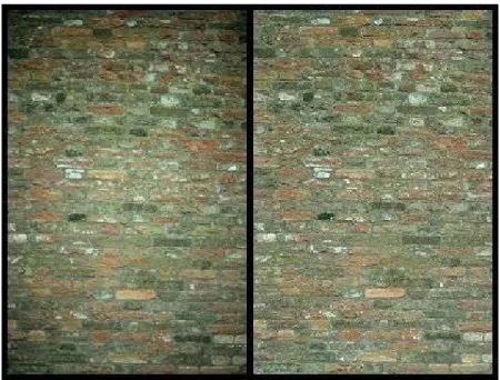
the scene’s appearance in images. The effects of the exposure change and vignetting

on images are shown in Figure 1.1. An image mosaic is created from multiple images,

where each image is taken with a different exposure value to capture the high dynamic

range of the scene, which is much greater than the camera’s dynamic range. While

the scene itself was reflecting light consistently during the image capture, the resulting

mosaic exhibits significant brightness inconsistency due to the exposure changes and

the vignetting effect. Another example of the effect of the exposure change is shown

in Figure 1.2, where pixel values of a point over time recorded with auto-exposure are

compared with those recorded with a fixed exposure value. In such outdoor scenes, the

exposure is adjusted to accommodate the significant lighting variation over the course

(16)

Figure 1.1: Effect of exposure and vignetting on images. Due to vignetting and exposure changes between images, there are significant brightness inconsistency in the image mosaic.

goes on the radiance of the points in the scene decrease, as shown by the pixel values

of the fixed exposure sequence. But the camera compensates for the decrease in the

brightness of the scene by increasing its exposure value, resulting in almost constant

pixel values over time.

While the exposure change (or auto-exposure) is desirable to make optimal use of

the limited dynamic range of most cameras, it has an ill effect on many computer vision

methods along with the nonlinearity of the camera response that rely on the scene

radiance measurement such as photometric stereo, color constancy, and on the methods

that use image sequences or time-lapse data of a long period of time such as in Jacobs

et al. (2006, 2007) and Weiss (2001) since the pixel values do not reflect the actual scene

radiance. The radiometric properties of the camera also affect the synthesis of image

mosaics and texture-maps for 3-D models from multiple images as seen in Figure 1.1. The

goal of this dissertation is to compute the radiometric properties of the cameras including

the radiometric response function, the exposure values, and the vignetting function from

multiple images which explain the relationship between the image brightness and the

(17)

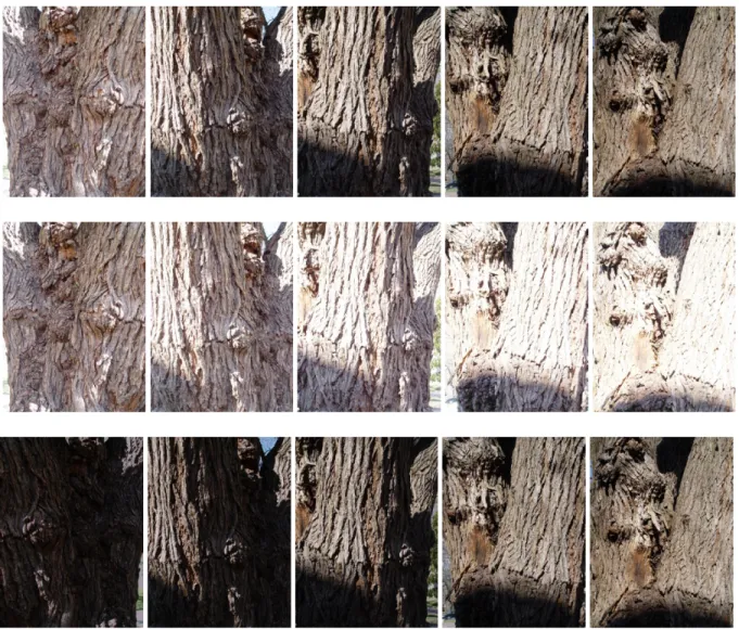
Figure 1.2: Effect of auto-exposure on images. Sample of images taken at different times with (Top) auto-exposure and (Middle) exposure fixed. (Bottom) Pixel values of a point over time.

1.1 Thesis Statement

Given a collection of images of a scene taken under varying conditions, one can

com-pute radiometric properties of the camera (up to some ambiguities) that explain the

relationship between the image brightness and the scene radiance as well as the

radio-metric relationship between multiple images. The radioradio-metric properties include the

radiometric response function, exposures, and vignetting.

1.2 Contribution

My research makes the following contributions:

1. Robust radiometric calibration and vignetting correction from corre-spondence. (Chapter 3)

(18)

func-tion, exposures, and the vignetting effect given multiple images taken with a freely

moving camera. Specifically,

• I present a method to decouple the vignetting effect from the radiometric

response function estimation.

• I introduce a novel method to estimate the radiometric response function from correspondences between images which is robust to noise and outliers

enabling the use of images from a moving camera.

• I present a vignetting estimation method which is also robust to noise and

outliers.

• I demonstrate methods to radiometrically align images and to create high

dynamic range (HDR) mosaics using the estimated radiometric properties of

the camera.

2. Joint feature tracking and radiometric calibration. (Chapter 4)

I present an algorithm suited for video data taken with auto-exposure where the

correspondence (feature tracks) and the radiometric response function along with

the exposure values are computed simultaneously. In detail,

• I present a novel method to simultaneously compute the feature tracks and

the camera exposure values from a video taken with a camera with known

response.

• I present a method to simultaneously compute the feature tracks, the

radio-metric response function, and the exposures from a video taken with a camera

with unknown response.

• I apply the results of the algorithm to build an adaptive stereo system.

(19)

I introduce a new algorithm to compute the radiometric response function and the

exposure of images given a sequence of images of a static outdoor scene taken over

time where the illumination is changing. In detail,

• I present a method to cluster pixels with same illumination conditions.

• I introduce a method to estimate the radiometric response function using the

group of pixels with same illumination conditions.

• I present a novel method to compute the exposure values of images using the illumination model assuming the known motion of the sun.

1.3 Overview

The remainder of the dissertation is organized as follows.

Chapter 2 presents the overview of the image formation process and the related

termi-nology. In addition, previous work on radiometric calibration and vignetting correction

is surveyed.

Chapter 3 describes a novel method for robust radiometric calibration and vignetting

correction that deals with images taken with a moving camera. Applications including

radiometric alignment of images for texture-mapping 3-D models and image mosaics as

well as high dynamic range (HDR) mosaic are shown.

Chapter 4 introduces a new framework for feature tracking where radiometric

cali-bration process is combined with feature tracking. The presented method is applied to

build an adaptive stereo system.

Chapter 5 presents a new algorithm to compute the radiometric response function

and the exposure of images given a sequence of images of a static outdoor scene where

the illumination is changing.

Chapter 6 discusses the contributions of this thesis and suggests directions for future

(20)

Chapter 2 Background

What determines the brightness at a certain point in an image? How is the image

brightness related to the actual scene brightness? These are the key questions asked for

this dissertation. Before presenting novel methods developed to answer those questions,

I first review the related terminology and the image formation process in this chapter. In

addition, a survey of previous work on the topic of radiometric calibration and vignetting

correction is presented.

2.1 Image Formation

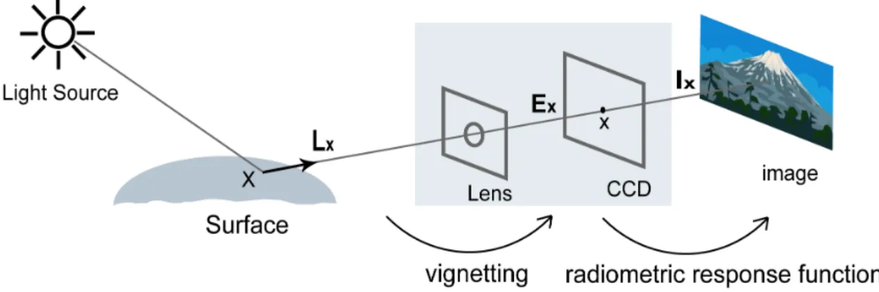
Figure 2.1 summarizes the image formation process. The scene brightness or the amount

of light reflected from a surface point (x) to a direction can be defined by the term

radiance which is the power per unit foreshortened area emitted into a unit solid angle

by a surface (Figure 2.1,L) (Horn, 1986). The unit for radiance is watts per square meter per steradian1 ₍_{W m}−2_sr−1_{). For a Lambertian surface for which the radiance leaving} the surface is independent of the angle, the radiance is proportional to the albedo of the

surface point and the dot product between the illumination direction and the surface

normal. Albedo is a reflectance term for Lambertian (diffuse) surface ranging from 0 to

1 characterizing the ratio of reflected light to incident light.

(21)

Figure 2.1: Radiometric image formation process. Vignetting affects the transformation from the scene radiance (L) to the image irradiance (E). Then the radiometric response function explains the nonlinear relationship between the image irradiance (E) and the image brightness (I).

After passing through the lens system, the power of radiant energy falling on the

image plane is called the image irradiance (Figure 2.1, E). The unit for irradiance is watts per square meter (W m−2_{). Irradiance is then transformed to image brightness (}_I_). These two steps, radiance to image irradiance and image irradiance to image brightness

are explained in more details below.

2.1.1 Radiance to Image Irradiance

The amount of light hitting the image plane (image irradiance,E) is proportional to the scene radiance (L) but varies spatially causing the fade-out in the image periphery due to multiple factors (Figure 2.2). This irradiance fall-off effect often goes unnoticed unless

the object in the image is of uniform color / brightness. However, this image distortion

can be damaging to photometric methods such as shape from shading, appearance-based

techniques such as object recognition, and image mosaicing (Zheng et al., 2006).

One of the factors for the irradiance fall-off in the periphery is the cosine-fourth law

(22)

1986). The following equation shows that the irradiance is proportional to the radiance

but it decreases as cosine-fourth of the angle θ that a ray makes with the optical axis. In the equation, R is the radius of the lens andd denotes the distance between the lens and the image plane.

E = LπR 2_cos4_θ

4d2 (2.1)

A more dominant source for the irradiance fall-off is a phenomenon called vignetting.

The vignetting effect refers to the gradual darkening of an image towards image corners

due to the blocking of a part of the incident ray bundle by the effective aperture size (Yu,

2004). The effect of vignetting increases as the size of the aperture increases and vice

versa (Figure 2.2). The white openings in Figure 2.2 indicate effective apertures. For

a large aperture size (small F-number), the opening is smaller when viewed from an

oblique angle because the view is blocked by the lens barrel. This implies that for large

apertures, the lens will collect less light away from its optical axis making the image

corners darker than its center. The vignetting effect decreases as the aperture size gets

smaller since the opening (effective aperture) gets smaller and no longer blocked.

A phenomenon called the pupil aberration has been described as another cause for

the fall in irradiance away from the image center (Aggarwal et al., 2001). The pupil

aberration is caused by the nonlinear refraction of the rays which results in a significantly

nonuniform light distribution across the aperture.

In this thesis, I view vignetting as the combination of all irradiance fall-off effects

including the effect from the cosine-fourth law and the pupil aberration as it is the most

dominant factor as well as to conform with the previous work and for generality. Rather

than trying to model this radiometric distortion physically by combining the effects from

different sources, we use a model that explains the overall irradiance fall-off behavior.

The following equation shows the mapping from radiance (LX) to image irradiance (Ex)

through the vignetting function (V(rx)) which is radially symmetric with r being the

(23)

(24)

Ex=V(rx)LX (2.2)

2.1.2 Image Irradiance to Image Brightness

The amount of light collected by the imaging sensor (irradiance E) is transformed to image brightness value (I) through a function called the radiometric response function or the camera response function. The relationship can be stated as follows :

Ix =f(kEx) (2.3)

where Ex is the image irradiance at a point x, k is the exposure value with which

the picture was taken, and Ix is the observed image intensity value at the pixel x.

Because increasing the irradiance will result in increasing (or keeping constant) the

image intensity for cameras, the response function is (semi-) monotonic and can be

inverted.

In general, the camera response is a nonlinear function providing means to compress

the dynamic range of the scene that far exceeds the dynamic range of the camera. For

digital cameras, even though the CCD and the CMOS respond linearly to the image

irradiance, nonlinearities are purposely introduced in the cameras electronics to mimic

the nonlinearities of film, to mimic the response of the human visual system, or to create

a variety of aesthetic effects (Grossberg and Nayar, 2004).

As can be seen in Equation (2.3), the exposure valuekplays a big role in deciding the final image intensity value by determining the amount of light exposed on the imaging

sensor. Since the dynamic range of the scene usually exceeds that of a camera, the

exposure value has to be adjusted to capture the dynamic range of interest by controlling

the shutter speed and/or the aperture. The shutter speed controls how long the imaging

(25)

Figure 2.3: Reciprocity : the same amount of light is obtained with an exposure twice as long and an aperture area half as big

1/60, 1/30, 1/15, and 1/8. The shutter speed affects how motions in the scene are

captured in the image: a fast shutter speed will freeze the movement and a slow shutter

speed will blur the motion. The aperture is the diameter of the lens opening which is

expressed as a fraction of focal length (f-number) such as f/2.0, f/2.8, f/4, f/5.6, etc.

Smaller f-numbers represent bigger apertures. The aperture is related to the depth of

field which means the amount of the picture, from foreground to background, that is

in sharp focus. A smaller aperture will give you a greater depth of field and a larger

aperture will give you a more restricted depth of field. Many different combinations of

the shutter speed and the aperture result in identical exposure2 _{and the choice depends} on the motion and the depth of field.

Most of the digital cameras provide several ways to set exposure. In the

auto-exposure mode, the camera automatically determines the appropriate aperture and

shut-ter speed for the scene. In addition, there are two semi-automatic methods called the

aperture priority mode and the shutter priority mode. In case of the aperture priority

(26)

mode, the user manually chooses the size of the aperture while the camera

automati-cally determines the shutter speed appropriate for the shooting condition. In the shutter

priority mode, the decision on the shutter is made by the user and the aperture is

de-termined by the camera. Finally, there is the manual mode in which both the aperture

and the shutter speed is manually chosen by the user.

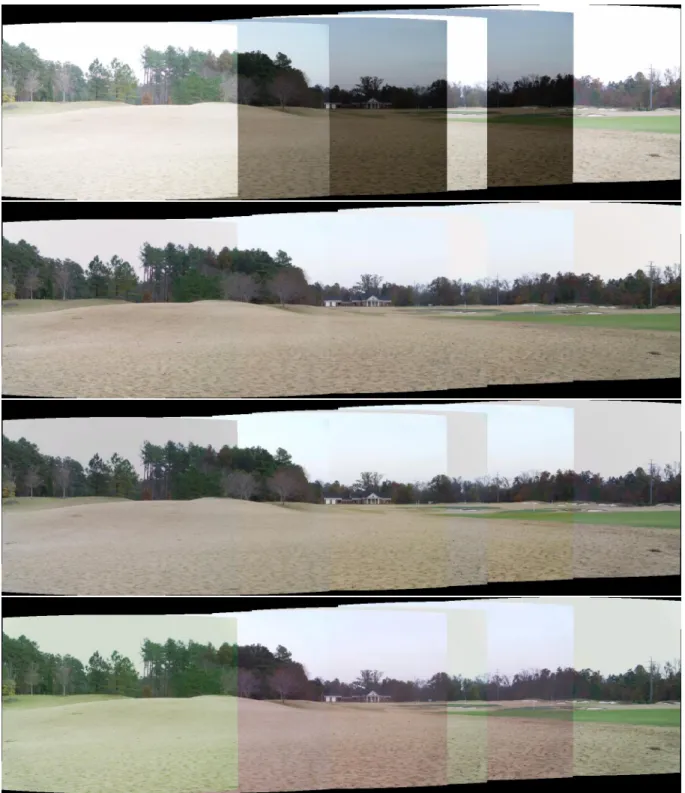
The effect of exposure change on images is illustrated in Figure 2.4. A set of images

were taken around a tree with auto-exposure where some images were taken inside

shadows and some in sunlight (images on top in Figure 2.4). The exposure value was

adjusted to a high value in shadows to allow more light in the camera and to a low

value in sunlight to allow less light. If the images were taken with a fixed low exposure,

the images will look as the images in the second row of Figure 2.4. On the other hand,

the images will look as the images on the bottom of Figure 2.4 if a fixed high exposure

was used. As can be seen, the auto-exposure functionality provides the flexibility of

not having to worry about finding the right 8-bit range to avoid over-exposed or

under-exposed images. However, the exposure change causes the appearance of the object

to change, which may be problematic for some computer vision methods that relate

multiple images, such as image matching, feature tracking, and creating image mosaics

and texture-maps.

There is another step in the imaging process called the white balance that influences

the image brightness. The white balance corresponds to color constancy in human visual

system, which is the ability to perceive color of an object independent of the

illumina-tion condiillumina-tion. The goal of white balance is usually to make sure that a white object

appears white in the image no matter what the illumination condition is (Martinkauppi,

2002). For example, a photograph taken under incandescent illumination will appear

unnaturally orange without proper white balance (Hsu et al., 2008). As with the

expo-sure, digital cameras provide automatic white balancing. One of the basic algorithms

(27)

(28)

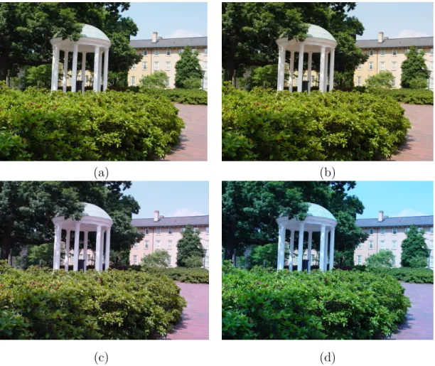
(a) (b)

(c) (d)

Figure 2.5: Effect of white balance. Photographs taken with different white balance set-tings (Sony F717) : (a) automatic white balance, (b) set to sunlight (c) set to fluorescent light (d) set to incandescent light.

average color in a scene is gray (Buchsbaum, 1980). Additionally, users can manually

adjust the white balance by setting the illumination condition to one of camera-provided

presets, such as daylight, cloudy, fluorescent, and incandescent. Figure 2.5 illustrates

the effect of white balancing with images taken with different white balance settings. In

this dissertation, the white balance is modeled with different exposure values for each

(29)

Figure 2.6: Macbeth color chart with 24 color patches with known reflectance.

2.2 Previous Work

While both the radiometric response function and the vignetting problem need to be

addressed to fully explain the radiometric image formation process, works on these two

problems have been developed separately in most cases. Hence, we can classify previous

work on the subject into three categories: methods that deal with the camera response

function only, methods that deal with vignetting only, and those that include both

problems.

2.2.1 Radiometric Response Function Estimation

We first discuss the works that compute the radiometric response function without

considering the vignetting effect. One way to compute the camera response function

is to photograph a color chart with known reflectances, such as the Macbeth chart

(Figure 2.6), in a uniform illumination condition. A mapping from the known reflectance

to the image intensity provides a simple means to find the camera response function.

However, the radiometric calibration using the color chart is not practical since the

method can be used only when the image of the chart is available.

(30)

calibration methods uses multiple images taken with different exposure values to

com-pute the camera response function. Assuming constant irradiance value, which implies

constant illumination while the photographs are taken, the change in intensity is

ex-plained by the change in exposure. Taking the inverse of the response function on both

sides in Equation (2.3), we get

f−1(Ix) =kEx . (2.4)

With two images taken with different exposure values ki and kj, Equation (2.4)

becomes

f−1₍_I

xi)

f−1₍_I

xj)

= ki

kj

, (2.5)

assuming the irradiance of the point stays constant (Exi = Exj). Let g = logf

−1 _and

K = logk, then we get the following relationship in the log-domain :

g(Ixi)−g(Ixj) = Ki−Kj . (2.6)

Equation (2.5) or (2.6) serves as the basis for computing the camera response function

in most of the methods that use multiple images taken with different exposures and the

early radiometric calibration methods concentrated on using different models of the

response function. Mann and Picard (1995) estimated the response curve assuming

that the response is a gamma curve and they know the exposure ratios between images.

While the method is limited due to the model of the response function, the work by Mann

and Picard has significance as the earliest work to introduce radiometric calibration from

images and the concept of extending the dynamic range by combining differently exposed

images. Debevec and Malik (1997) introduced a nonparametric method for response

function recovery by imposing a smoothness constraint and assuming that the exposure

(31)

range (HDR) radiance maps from multiple images with different exposures, and showed

applications of HDR maps such as synthesizing realistic motion blur and simulating the

response of the human visual system. In the work by Mitsunaga and Nayar (1999),

the response curve was assumed to be a low degree polynomial and was estimated

iteratively with rough exposure ratio estimates. In their work, Mitsunaga and Nayar

also introduced a method for automatic rejection of image areas with large vignetting

effects and fused multiple images for HDR imaging. Tsin et al. (2001) also introduced an

iterative method for computing the response function with the nonparametric response

form using a statistical model of the measurement errors. Pal et al. (2004) propose

the use of probability models for the imaging system and prior models for the response

function to estimate the response function that is modeled differently for each image

in the sequence. In Grossberg and Nayar (2004), the authors introduced a new model

for the response function called the empirical model of response (EMoR) which is based

on applying principal component analysis (PCA) to the database of response functions.

This model will be discussed in details later in this chapter. A common limitation of all

the mentioned methods above is that both the camera and the scene have to be fixed

when multiple images are photographed for the calibration.

Several methods were introduced to loosen the scene and the camera movement

re-strictions. Mann and Mann (2001) proposed an iterative method with a non-parametric

model that computes the response function and the exposures that allows camera

ro-tation. Grossberg and Nayar (2003) explained ambiguities associated with the problem

of finding the response function and introduced a response curve estimation method by

recovering intensity mapping functions3 _{between differently exposed images from} his-tograms using histogram specification. The registration process is unnecessary in this

method, allowing small movement of the scene and the camera. In Candocia and

Man-3_{In this dissertation, I use the term} _{brightness transfer function} _{instead of the intensity mapping}

(32)

darino (2005), the authors present an approach for response function computation by

approximating the camera response function with a constrained piecewise linear model.

They also incorporate the framework for spatial and tonal image registration (Candocia,

2003) to allow camera rotation.

Methods described so far use multiple images taken with different exposures and

assume the irradiance for each image point stays constant, which implies that the

illu-mination condition for all the images in the sequence is the same. A couple of methods

were presented for computing the camera response when the illumination is changing.

Manders et al. (2004) proposed a radiometric calibration method by using superposition

constraints imposed by different combinations of two (or more) lights. It is difficult to

apply this method in practice because it requires two or more images, each with

differ-ent lighting direction, and an image with all the lights combined. Shafique and Shah

(2004) also introduced a method that uses differently illuminated images. They estimate

the response function by exploiting the fact that the material properties of the scene

should remain constant and use cross-ratios of image values of different color channels

to compute the response function. The response function is modeled as a gamma curve

and a constrained non-linear minimization approach is used for the computation. This

method is also limited in practice due to the restricted model for the response function

and the algorithm is verified only by synthetic experiments by the authors.

Instead of using multiple images with different exposures or different lighting

con-ditions, there are algorithms that compute the camera response function from a single

image. Farid (2001) treats the radiometric nonlinearity as a gamma correction and

presents a technique for computing the gamma correction from a single image without

any information about the imaging device. His approach exploits the fact that gamma

correction introduces specific higher-order correlations in the frequency domain which

can be detected using tools from polyspectral analysis. The method by Farid is limited in

(33)

Figure 2.7: An image of a flat and textureless Lambertian surface under constant illu-mination can be used as an reference image for vignetting estimation.

In the work by Lin et al. (2004), a single image was used for computing the response

function by looking at the color distributions of local edge regions. Measured colors

across edges should form linear distributions in color space due to blending of distinct

region colors. However, they actually show nonlinear distributions because of the

non-linear camera response function. Using this idea, Lin et al. (2004) compute the response

function which maps the nonlinear distributions of edge colors into linear distributions.

Lin and Zhang further extended the method to deal with a single grayscale image by

using the histograms of edge regions (Lin and Zhang, 2005). While these methods can

be used for cases when multiple images with different exposures are not available, they

are susceptible to high levels of image noise. Matsushita and Lin (2007) presented a

method to complement the methods in Lin et al. (2004) and Lin and Zhang (2005) by

using the asymmetric profiles of measured noise distributions to compute the camera

response function which maps the asymmetric noise distribution to a symmetric

dis-tribution. This method requires the noise distributions for different image irradiances,

which may not be simple, and the assumption on the symmetric noise distribution may

(34)

2.2.2 Vignetting Estimation

We now discuss previous work on vignetting. Conventional methods for correcting

vi-gnetting involve taking a reference image of a non-specular object such as a white paper

with uniform color (Figure 2.7). This reference image is then used to build a correction

lookup table or to approximate a parametric correction function. Asada et al. (2001)

proposed a camera model using a variable cone that accounts for vignetting effects in

a zoom lens system. Parameters of the variable cone model were estimated by taking

images of a uniform radiance field. Yu et al. proposed using a hypercosine function

to represent the pattern of the vignetting distortion for each scanline (Yu et al., 2004).

They expanded their work to a 2D hypercosine model in Yu (2004) and also introduced

an anti-vignetting method based on wavelet denoising and decimation. Other vignetting

models include a simple form using radial distance and focal length (Uyttendaele et al.,

2004), a third-order polynomial model (Bastuscheck, 1987), a first order Taylor

ex-pansion (Sawchuk, 1977), and an empirical exponential function (Chen and Mudunuri,

1986). While above methods rely on a reference image of an object of uniform color,

Zheng et al. introduced a new method for determining the vignetting function given

only a single image of a normal scene (Zheng et al., 2006). To extract vignetting

in-formation from an image, they presented adaptations of segmentation techniques that

locate image regions for vignetting estimation. In all of the works mentioned above,

the radiometric response function was ignored and vignetting was modeled in the image

intensity domain rather than in irradiance domain.

In a related work, Schechner and Nayar (2003) exploited the vignetting effect to

capture high dynamic range intensity values. In their work, they calibrate the ”intended

vignetting” using a linear least-squares fit on the image data itself rather than using a

reference image. Their work assumes either a linear response function or a known

response function. In Kang and Weiss (2000), vignetting effect was used for camera

(35)

addition to the vignetting effect. Using an image of a flat and textureless Lambertian

surface under constant illumination, the camera intrinsics such as focal length, principal

point, aspect ratio, and skew were computed. While the concept was novel, their method

was impractical, since it did not yield accurate calibration results with real images.

2.2.3 Radiometric Response Function and Vignetting

Estima-tion

Recently, works that include both the radiometric response function and the vignetting

effect have been introduced. Litvinov and Schechner presented an unified framework for

simultaneously estimating the unknown response function, exposures, and vignetting

from a normal image sequence taken with camera motion (Litvinov and Schechner,

2005a,b). They achieve the goal by a nonparametric linear least squares method using

common areas (correspondences) between images. Goldman and Chen (2005) also

pre-sented a solution for estimating the response function, the exposures, and vignetting.

Using the empirical model of response (EMoR, Grossberg and Nayar (2004)) for the

re-sponse function and a polynomial model for vignetting, they estimate the model

parame-ters simultaneously by a nonlinear optimization method. In these papers, the recovered

response function, exposure, and the vignetting factors were used to radiometrically

align images for seamless mosaics. The method presented in Chapter 3 falls into this

category and the results will be compared with results from Litvinov and Schechner

(2005a) and Goldman and Chen (2005).

2.3 Radiometric Response Function Model

Before introducing different methods for radiometric calibration, I will first introduce the

model of the radiometric response function used through out the dissertation. To model

(36)

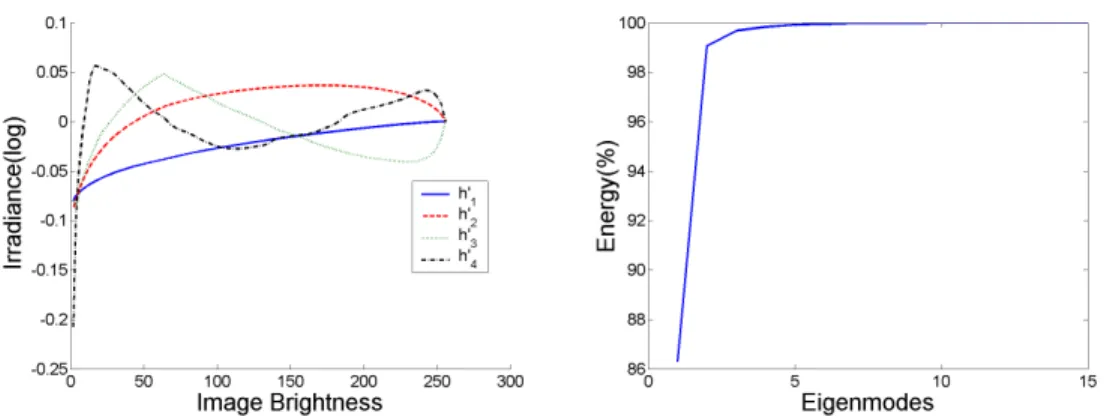
Figure 2.8: EMoR Basis. (Left) First four basis of the DoRF (log space), (Right) The cumulative energy occupied by the first 15 basis

Grossberg and Nayar (2004) will be used. In their work, Grossberg and Nayar first show

that all response functions must lie within a convex set that results from the intersection

of a hyperplane and a positive cone in function space. They also collected a Database

of Response Functions (DoRF) of a variety of imaging systems including film, CCD,

and solid-state camera components that are currently used. The database includes a

total of 201 real-world response functions. Then they combine the constraints from the

theoretical analysis and the data from DoRF to formulate a new model for the camera

response function called the Empirical Model of Response (EMoR) which is a low (Mth₎

order approximation :

f(E) = f0(E) +

M X

n=1

cnhn(E), (2.7)

wherehn’s are basis functions found by applying PCA to the DoRF and f0 is the mean function.

In log space, Equation (2.7) becomes :

g(I) =g0(I) +

M X

n=1

cnh0n(I), (2.8)

where g(I) = lnf−1₍_I_{) and} _h0

(37)

the database. The h0_n’s are found by applying PCA to the log space of the DoRF. One thing to notice is that elements of the first column and the first row of the covariance

matrix of DoRF in log space are -∞ since data are normalized from zero to one. So,

we remove the first column and the first row from the matrix for the PCA. Figure 2.8

shows the first four basis functions of the log space of DoRF and the cumulative energy

occupied by first 15 basis. The first three eigenvalues explain more than 99.6%, which

(38)

Chapter 3 Robust Radiometric Calibration and

Vignetting Correction from

Correspondence

3.1 Introduction

In this chapter, I introduce an algorithm to compute the vignetting function, the

re-sponse function, and the exposure values that fully explain the radiometric image

forma-tion process from a set of images of a scene taken with different and unknown exposure

values. One of the key features of the method is that the movement of the camera is not

limited when taking the pictures whereas most existing methods limit the motion of the

camera. The main application of interest is to radiometrically align images for image

mo-saics and for texture mapping 3D models where vignetting and exposure changes cause

color inconsistency. The proposed approach is essentially different from image

blend-ing/feathering methods commonly used in image mosaicing (Brown and Lowe, 2003;

Burt and Adelson, 1983; Levin et al., 2004) and other texture correction methods such

as the method in Jia and Tang (2005) where the global and the local intensity variation

were corrected using tensor voting, the method in Agathos and Fisher (2003) where a

(39)

Beauchesne and Roy (2003) where a common lighting between textures was derived to

relight textures. I also apply the method to create high dynamic range (HDR) mosaics

that better represent radiometric measurement of the scene than normal mosaics.

The rest of the chapter is organized as follows. In the next section, a novel method

for computing the radiometric response function is introduced. In Section 3.3, an

al-gorithm for vignetting estimation is presented. Associated ambiguities are explained in

Section 3.4 and methods for radiometrically aligning images and creating HDR mosaic

are presented in Section 3.5. The proposed method is evaluated with various

experi-ments in Section 3.6 and the chapter is concluded with discussions about the algorithm

in Section 3.7.

Versions of this work were published in Kim and Pollefeys (2004) and Kim and

Pollefeys (2008).

3.2 Radiometric Response Function Estimation

We begin by showing the equations for relating radiance (L) to image irradiance (E) and image irradiance (E) to image brightness (I) as introduced in Chapter 2.

Ex=V(rx)LX (3.1)

Ix =f(kEx) (3.2)

Combining (3.1) and (3.2), the radiometric process of image formation can be

mathe-matically stated as follows.

Ix=f(kV(rx)LX) (3.3)

LX is the radiance of a scene point X towards the camera, Ix is the image intensity

(40)

from the center of vignetting. We assume that vignetting is radially symmetric with the

center of vignetting being the center of the image. We also assume that the vignetting

function is the same for all images in the sequence. Equation (3.3) can be rewritten as

follows.

ln(f−1(Ix)) = lnk+ lnV(rx) + lnLx (3.4)

g(Ix) =K+ lnV(rx) + lnLx (3.5)

The goal of our algorithm is to estimate f() (or g()), V(), and k (or K) given a set of differently exposed images taken with a non-stationary camera. Our work

falls under the last group of existing work (Goldman and Chen (2005); Litvinov and

Schechner (2005a)) explained in the previous chapter where both the response function

and the vignetting function are recovered. The difference between those methods and

our method is that while the camera response function and the vignetting function were

estimated simultaneously in Goldman and Chen (2005) and Litvinov and Schechner

(2005a,b), we approach the problem differently by robustly computing the response

function and the vignetting function independently. Separating the two processes is

possible by decoupling the vignetting process from the radiometric response function

estimation. By separating the two processes, we derive a solution for each process that

is robust against noise and outliers. Thus we are able to get robust estimation even

when there is a vast number of outliers due to inaccurate stereo correspondences for

the overlap region on the 3D models as well as non-Lambertian reflection. Previous

least-squares based approaches are not able to deal with this.

3.2.1 Correspondence

Since we are dealing with images taken with a moving camera, the first thing that

we consider is the computation of correspondences. Ideally, only a limited number of

(41)

vignetting parameters. However, because of a certain number of limitations in finding

accurate correspondences, it is best to estimate correspondences for a larger number of

points. First, we want corresponding points to cover as many intensity values as possible

(and this for each R, G and B channel separately). In addition, matching between images

recorded with different exposure settings is in itself hard, thus, we expect a significant

number of wrong matches. Finally, because we deal with a moving camera and not

all pixels correspond to Lambertian surfaces, we can not always expect the radiance to

be constant over varying viewing directions (this would not be a problem for static or

purely rotating cameras). Therefore, it is important to obtain as much redundancy as

possible so that a robust approach can later be used to estimate the desired camera

properties.

If the set of images are captured with a purely rotating camera, we compute the

homographies between images to compute the correspondences. We used the software

”Autostitch” (Brown and Lowe, 2003)1 for computing the homographies.

For images taken with a moving camera, the correspondences are computed by

esti-mating the epipolar geometry for each pair of consecutive images (for video, keyframes

would be selected so that the estimation of the epipolar geometry would be stable) using

tracked or matched features, followed by stereo matching (Pollefeys et al., 2004). To

avoid problems with intensity changes it is important to use zero-mean normalized

cross-correlation. While we do not explicitly deal with independent motions in the scene, our

stereo algorithm combined with our robust joint histogram approach explained in the

next subsection will handle those as outliers.

3.2.2 Estimating the radiometric response function

Equation (3.3) shows that the response function f() cannot be recovered without the knowledge about the vignetting function V() and vice versa. Hence, one way to solve

(42)

the problem is to estimate both functions simultaneously either in a linear (Litvinov and

Schechner, 2005a,b) or in a nonlinear way (Goldman and Chen, 2005) . But if we use

corresponding points affected with the same amount of vignetting, we can decouple the

vignetting effect from the process and estimate the response function without worrying

about the vignetting effect using Equation (3.3). Letxiandxj be image points of a scene

point X in image i and image j respectively. If rxi =rxj then V(rxi) =V(rxj) since we have already made the assumption that the vignetting model is the same for all images

in the sequence. Hence by using corresponding points that are of equal distance from the

center of each image, we can decouple vignetting from the response function. So after

finding all possible correspondences first using the methods described in the previous

subsection (homography for rotating camera and stereo matching for moving camera),

we then compare the distance of the points in each matching pair from the center of

its image in order to select only correspondences with equal distance. In practice, we

allowed some tolerance to the constraint by allowing correspondences that are close to

equal distance from the center rather than strictly enforcing correspondences to be of

exact equal distance. In the case of panoramic images, these correspondences will form

a band between images (Figure 3.1). In the case of stereo images, these correspondences

will form an arbitrarily deformed shape depending on the geometry of the scene and the

motion of the camera (Figure 3.2). Note that while in general there are no problems

finding a sufficient amount of such correspondences in stereo cases, there are some cases

that may not yield enough correspondences particulary in the case of forward (backward)

motion where the radius for all pixels would increase (decrease) (except that even in that

case we might still have far away points that stay approximately fixed and allow for the

exposure changes to be computed while the response function mostly gets constrained

by other images).

By using only those correspondences mentioned above, we obtain the following

(43)

Figure 3.1: Decoupling the vignetting effect (mosaic image) : The figure shows three images stitched to a mosaic. Only corresponding points in the colored band (red for the first pair and blue for the second) are used to decouple the vignetting effect from estimating the radiometric response function .

(a) (b)

(c) (d)

(44)

Figure 3.3: An example of a joint histogram with the estimated brightness transfer function (BTF) overlaid on it.

g(Ixi)−g(Ixj) =Ki−Kj (3.6) While Equation (3.6) is solved for the response function g() in a least squares sense in most previous works, we approach the problem in a robust way to achieve robustness

against noise and mismatches. This is very critical since we are dealing with images

taken with a moving camera where using least squares would not yield accurate results

due to noise and a vast number of outliers. The robust estimation process is explained

in details in the following subsections.

Joint Histogram and Brightness Transfer Function

For a pair of images, all the information relevant to our problem is contained in the

pair of intensity values of corresponding points. As suggested in Mann (2000), these can

all be collected in a two-variable joint histogram which he calls the comparagram. For

(45)

toIxj.

As noted in Grossberg and Nayar (2003), ideally a function should relate the intensity

values between the two images. From Equation (3.6), one immediately obtains

Ixj =τ(Ixi) := g

−1

(g(Ixi) + ∆K) . (3.7)

with ∆K = Kj −Ki. We will call the function τ as the brightness transfer function

(BTF). It was shown in Grossberg and Nayar (2003) that under reasonable assumptions

for g, τ is monotonically increasing,τ(0) = 0 and if ∆K >0, then I ≤τ(I). Inversely, if ∆K < 0 then I ≥ τ(I). Ideally, making abstraction of noise and discretisation, if

Ixj 6= τ(Ixi), then we should have J(Ixi, Ixj) = 0. However, real joint histograms are quite different due to image noise, mismatches, view dependent effects and a non-uniform

histogram as shown in Figure 3.3. In the presence of large numbers of outliers, least

squares solutions for response functions as have been used by others are not viable. We

propose to use the following function as an approximation for the likelihood of the BTF

passing through a pixel of the joint histogram.

P(τ(I1) =I2|J¯) = (G(0, σ1)∗J¯)(I1, I2) +Po (3.8)

where G(0, σ1)∗ represent the convolution with a zero-mean Gaussian with standard deviationσ1 to take image noise into account, ¯J is the normalized joint histogram, and

P0 is a term that represents the probability for τ(I1) = I2 independent of the joint histogram. This term is necessary to be able to deal with the possibility of having the

BTF pass through zeros in the joint histogram which could be necessary if for some

intensity values no correct correspondence was obtained. Based on these assumptions

the most probable solution is the BTF that maximizes

lnP(τ|J¯) =

Z Z

(46)

with Jτ(I1, I2) being a function that is one where I2 =τ(I1) and zero otherwise. Using dynamic programming it is possible to compute the BTF that maximizes Equation (3.9)

under the constraints discussed above, i.e. semi-monotonicity, τ(0) = 0, τ(255) = 255 and τ(I)≥I or τ(I)≤I for all I (Figure 3.3).

3.2.3 Radiometric Response Function Estimation

With the computed BTFs, we now estimate the radiometric response function by using

the low parameter Empirical Model of Response (EMoR) by Grossberg and Nayar (2004)

as the model for the response function which was explained in Section 2.3. The equation

for the model in log space is as follows.

g(I) =g0(I) +

M X

n=1

cnh0n(I), (3.10)

where g(I) = lnf−1(I) and h0_n’s are basis functions for log inverse response function of the database.

We estimate the response function and exposure differences between images by using

the computed BTFs and combining Equation (3.6) and Equation (3.10).

g0(τij(I))−g0(I) +

M X

n=1

cn(h0n(τi,j(I))−h0n(I))−Kji = 0 (3.11)

whereKji =Kj−Ki andτi,j() is the brightness transfer function from the image iwith

exposure Ki to the image j with exposure Kj.

To deal with the white balance, we adopt the simplifying assumption that the effect

of white-balance corresponds to changing the exposure independently for each color band

(Finlayson et al., 1994). Then the unknowns of Equation (3.11) are the coefficientscn’s

and the exposure differencesKji’s for each different color channel. The solution for these

unknowns at this point will suffer from the exponential ambiguity. The exponential

(47)

to Equation (3.6) then so are γg and γK’s. Simply put, there are many response functions and exposures that satisfy the equation as long as they have the same scale

factor. As stated in Grossberg and Nayar (2003), it is impossible to recover both the

response function (g) and the exposures (K’s) simultaneously from BTF alone, without making assumptions on either the response function or the exposures. To resolve this

ambiguity problem, we chose to make an assumption on an exposure value by setting

the exposure difference of a pair to a constant value (α). For simplicity, we will set the exposure difference of the first image pairK12 to a constant value (α) in this work. This serves as fixing the scale of the response function. For many applications including the

tonemapping for high dynamic range imaging and the texture alignment application,

the choice of the constant is not critical which is an advantage over many other methods

which require exact or rough estimate of exposure values. The sign of α should be positive when the exposure increases while it should be negative when the exposure

decreases for the chosen pair. Alternatively, the scale can be fixed by setting the value

of the response curve at an intensity to an arbitrary value. This alternative method is

used in Chapter 4 and Chapter 5 to deal with the ambiguity.

After fixing the value ofK12, we now have to solve for the unknown model parameters (cn) and exposure differences of each image pair for each color channel except the first

pair which amounts toM+ 3(N−2) unknowns. The computed BTF (τ) for each color channel of an image pair yields 254 equations (Equation 3.11) for image values (I) 1 to 254. We do not include the value 0 and 255 to avoid under-exposed or saturated data.

To solve the problem in a linear least squares sense, we first build matrices Al_i (254×(M+ 3(N −2))) and bl

(48)

(2≤i≤N −1) and each color channel (l ∈ {R, G, B} or{0,1,2}).

Al_i(m, n) =

          

w(m)(h0_n(τl

i,i+1(m))−h

0

n(m)); 1≤m≤254,1≤n ≤M

−w(m); 1≤m≤254, n=M+(N −2)×l+i−1 0; elsewhere

(3.12)

bl_i(m) =w(m)(g0(m)−g0(τi,il +1(m))); 1≤m ≤254 (3.13) For the first pair (i= 1),

Al₁(m, n) =



 

 

w(m)(h0_n(τl

1,2(m))−h

0

n(m)); 1≤m≤254,1≤n ≤M

0; elsewhere

(3.14)

bl₁(m) = w(m)(g0(m)−g0(τ1l,2(m)) +α); 1≤m≤254 (3.15) The weight w is as follows.

w(m) =w1(m)w2(m) (3.16)

w1(m) =



 

 

0; if J(m, τ(m))< or τ(m) = 0 or 255 1; else

(3.17)

w2(m) = exp(−

((m−127)/127)2 2σ2

2

) (3.18)

The weights are included for two reasons. First, joint histograms may not contain

data on all the intensity range. So the brightness transfer function (τ) values at the intensity range where there are no data (or very few) may not be accurate. Also, data

that are either saturated or under-exposed should be eliminated from the equation. All

these factors are reflected in the first weight w1.

In addition, the response function will typically have a steep slope near Imax and

Imin, so we expect the response function to be less smooth and fit the data more poorly

(49)

the second weight w2. We used values from 1.0 to 10.0 for σ2 for the examples in this chapter.

To deal with the discretization problem, we also compute BTFs in the opposite

direction (i+1 toi) and build matrices Al0

i and bl

0

i which is similar to Ali and bli except

that τi,i+1 is now changed toτi+1,i along with following few changes.

Al_i0(m, n) =

          

w(m)(h0_n(τl

i+1,i(m))−h

0

n(m)); 1≤m≤254,1≤n ≤M

w(m); 1≤m ≤254, n=M+(N −2)×l+i−1 0; elsewhere

(3.19)

bl_i0(m) =w(m)(g0(m)−g0(τil+1,i(m))); 1≤m ≤254 (3.20)

Al₁0(m, n) =



 

 

w(m)(h0_n(τ₂l_,₁(m))−h0_n(m)); 1≤m≤254,1≤n ≤M

0; elsewhere

(3.21)

bl₁0(m) =w(m)(g0(m)−g0(τ2l,1(m))−α); 1≤m≤254 (3.22) After all the matrices above are built, we can solve for the coefficients of the model

and the exposure differences linearly (Au = b) using the singular value decomposition (Equation (3.25)) by combining all the computed matrices to formA andb as in Equa-tion (3.23) where each Al _and _bl _{are formed by combining} _Al

i and bli for all image

(50)

A=                 AR

AR0

AG AG0 AB AB0

                b =                 bR

bR0

bG bG0 bB bB0

                (3.23)

u=c1, . . . , cM, K23R, . . . , K

G

23, . . . , K

B

23, . . . , K

B N−1N

T

(3.24)

ˆ

u= arg min

u kAu−bk2. (3.25)

3.3 Vignetting Estimation

After estimating the response function and the exposure values, each image intensity

value is transformed to an irradiance value E to compute vignetting function V.

Ex =

f−1₍_I

x)

k =V(rx)LX (3.26)

Since the scene radiance LX is the same for the corresponding points xi and xj, we

get

Exi

V(rxi)

= Exj

V(rxj)

(3.27)

As presented in Section 2.2.2, many models for vignetting exist. In this dissertation,

we chose to use the polynomial model used in Goldman and Chen (2005). In Goldman

and Chen (2005), a third order polynomial was used for the vignetting model and

it was estimated together with the response function simultaneously by a nonlinear

optimization method. By computing the response function independent of vignetting in

(51)

a great deal of computational time compared to the nonlinear optimization scheme used

in Goldman and Chen (2005), avoids issues with potential local minima, and it also

enables us to easily use much higher order polynomial function for more accuracy. The

vignetting model is given by

V(r) = 1 +

D X

n=1

βnr2n. (3.28)

Let a = Exi

E_xj, then combining the model with Equation (3.27) yields the following

equation.

D X

n=1

βn(ar2xnj −r

2n

xi) = 1−a (3.29)

One obvious choice for solving for the D unknown βn’s is to use least squares since

each corresponding pair of points in given image pairs provides additional equation in

the form of (3.29). But in the presence of many outliers, the least squares solution will

not give us a robust solution to the problem.

We propose to approach the problem similar to the way we computed the response

function in the first stage. Rather than solving the problem in a least squares sense, we

once again solve the problem in a robust fashion. For a pair ofrxi and rxj (discretized),

we estimate ˆa(rxi, rxj) which is the robust estimate of the ratio a for the given rxi and

rxj. For each matching pair of points in the image sequence with radius rxi and rxj

respectively, the irradiance ratio a is computed and stacked at s(rxi, rxj) (Figure 3.4).

We only use correspondences where the image intensity of each pixel is within certain

range, from 10 to 245 for example. The purpose of this is to exclude saturated or

under-exposed pixels as well as pixels in the intensity range where estimate of the response

function tends to be less accurate. Also, only pairs with similar ratio for each color

channel are added to the stack since the vignetting effect is the same for all color

channels. In the end, ˆa(rxi, rxj) is computed as the median of stacked values s(rxi, rxj) .

(52)

Figure 3.4: Estimating the irradiance ratio ˆa. For every matching pair with rxi = r1,

rxj = r2, the value a is stacked in s(r1, r2). ˆa(r1, r2) is computed as the median of stacked values.

the discretisation of 100×100, we have less then 5000 equations in the form of Equation (3.29) instead of having one equations per matching pair of points.

The model coefficients (v = [β1, β2, ..., βD]T) are estimated by solving the linear

equation of the form Yv = z. The mth _r

xi and rxj pair adds one equation (Equation (3.29)) to the linear equation as follows.

Y(m, n) = wv(m)(ˆa(rxi, rxj)r

2n

xj −r

2n

xi) (3.30)

z(m) =wv(m)(1−ˆa(rxi, rxj)), 1≤n ≤D

Note that we weight (wv) each row of the matrixY andzby the number of elements

in the stack s(rxi, rxj). Finally, the model parameter vector v is the solution to the

following least squares problem Equation (3.31) which can be solved using the singular

value decomposition (SVD).

ˆ

v= arg min

(53)

Once we have the estimates of the response, the exposures, and the vignetting

func-tion from the given set of images, we can add other images that may have different

exposure value and vignetting such as zoomed-in images to capture more dynamic range

and details. Assuming that the center of vignetting stays at the center of the image,

we can first compute the exposure of the added image using the pixels close to the

cen-ter that are not affected by vignetting (we used pixels within 10% from the cencen-ter) by

Equation (3.5). Then the vignetting function is computed robustly in a similar way as

the vignetting estimation described in the previous section. From Equation (3.27), the

vignetting function for the zoomed-in image (Mz) is computed with the known response

function (f), the vignetting function of the original image (Mi), the exposure of the

original image (ki), and the exposure of the zoomed-in image (kz) as follows.

Vz(rxz) =

f−1(Ixz)kiVi(rxi)

f−1₍_I

xi)kz

(3.32)

Again for the robustness against outliers and noise, we use the median of the

right-hand side value of Equation (3.32) for each radius to fit the vignetting model instead of

fitting the model to all possible data. An example of adding a zoomed-in image to the

sequence is shown in the experiments section (Figure 3.15).

3.4 Ambiguities

As mentioned earlier, the process of radiometric calibration explained thus far is subject

to the exponential ambiguity, sometimes called the γ ambiguity as in Grossberg and Nayar (2003) and Litvinov and Schechner (2005a). This ambiguity basically means that

if ˆf, ˆk, and ˆV are the solutions for Equation (3.3), then the whole family of ˆfγ_{, ˆ}_kγ_{, and}

ˆ

Vγ _{are also solutions to the problem. In this work, this ambiguity is dealt by setting an}

exposure ratio of an image pair to a constant value.

(54)

2005a) corresponding to arbitrary offsets in Equation (3.5) : g + Sg, K +SK, and

lnV(rx) +SV would all satisfy the equation with the radiance value being offset

ac-cordingly. This ambiguity is dealt with in this dissertation by normalizing the response

function and the vignetting function.

Due to these ambiguities, the radiance value ˆLx that we recover using Equation

(3.33) with the estimates f(), V(), and k would not be the true radiance value (Lx).

It would be related to the true radiance by an exponential function. However, this

is not a problem for many applications including the radiometric alignment and the

high dynamic range display explained in the next subsection unless absolute or linearly

proportional quantitative measurements are required such as in the simulation of motion

blur or lens glare effects (Debevec and Malik, 1997).

ˆ

Lx =

f−1(Ix)

kV(rx)

(3.33)

3.5 Radiometric Alignment and High Dynamic Range

Mosaic Imaging

After computing the response function (f()), the vignetting function (V()), and exposure values (k) for each image, we can radiometrically align images in the sequence so that the vignetting is corrected and all images have a common exposure setting as follows.

I_xnew =f(knewLˆx) (3.34)

The ambiguities mentioned above will not have any effect on the alignment since

the solutions with different γ values will still generate the same intensity values. By radiometrically aligning images, we can make mosaics and textures of 3D models look

(55)

under-exposed may still look inconsistent in the resulting mosaic or the 3D model depending on

the new exposure value. We cannot find the radiance value if a pixel is either saturated

or under-exposed.

Another application of our method is the high dynamic range (HDR) imaging,

specif-ically creation of the high dynamic range mosaic. Radiometrspecif-ically aligning images has

the effect of fixing the exposure which limits the showing of the full dynamic range of the

scene. By displaying the estimated scene radiance values ( ˆLx), we can represent the high

dynamic range scene more realistically. While we are not displaying the actual radiance

value due to ambiguities, we can alleviate the problem by tuning the value of γ for vi-sual plausibility (Litvinov and Schechner, 2005b). Since most of the displaying systems

cannot show high dynamic range images, we have to compress the estimated radiance

values ( ˆLx) appropriately using a method called tonemapping. In this dissertation, we

used a software called Photomatix2 for tonemapping.

For high dynamic range mosaics, we scan the scene changing the exposure

accord-ingly. We have to make sure that every point in the mosaic is at least once correctly

exposed meaning it is neither underexposed or saturated. The response function,

ex-posures, and vignetting are computed using our method and the approximate radiance

value in Equation (3.33) for each point is computed by averaging the estimated radiance

value ( ˆLx) of the point in multiple images. Pixels that are either saturated or

under-exposed are excluded in the averaging process. An HDR mosaic example is shown in

the next section.

3.6 Experiments

In this section, we evaluate the performance of our proposed method. We test our

algorithm by performing experiments with real data as well as synthetic data.

Radiometric calibration methods from image sequences