Queueing Approaches to Appointment System Design
Jianzhe Luo
A dissertation submitted to the faculty of the University of North Carolina at Chapel Hill in partial fulfillment of the requirements for the degree of Doctor of Philosophy in the Department of Statistics and Operations Research.
Chapel Hill 2012
Approved by:
Vidyadhar G. Kulkarni
Serhan Ziya
Scott Provan
Nilay T. Argon
c
2012
Jianzhe Luo
ABSTRACT
JIANZHE LUO: Queueing Approaches to Appointment System Design (Under the direction of Vidyadhar G. Kulkarni and Serhan Ziya)
We develop useful queueing models to analyze appointment-based service systems. There
are many factors that make appointment scheduling in service systems extremely complex.
For example, scheduled customers may not arrive on time or show up at all, customers with
different priorities may have conflict of service access, service may last shorter or longer than
expected, and so on. These kinds of uncertainties make stochastic modeling a perfect tool
to be used to analyze and improve the performance of such systems. The objective of our
research is to identify appointment scheduling policies that balance the utilization of
expen-sive service resources and customer waiting. We specifically consider two problems that have
been commonly observed in practice but received little attention from the past
appointment-scheduling literature. The first problem is how to schedule appointments when scheduled
services may be interrupted by service requests with higher priority. We generate the optimal
scheduling policies under various scenarios: finite and infinite time horizon, equally spaced
and non-equally spaced scheduling, constant and time-dependent interruption rate, and
pre-emptive and non-prepre-emptive service interruptions. In the second problem, we consider the
appointment system as two queues in tandem: the appointment queue followed by the service
queue. The customers join the appointment queue when they call for an appointment, stay
there (not physically) until the appointment time comes, and then leave the appointment
queue and physically join the service queue, and wait there until served. We explicitly
cap-ture the dependence between these two queues and derive important performance measures
of interest, such as service utilization and customer long-run average waiting times in both
ACKNOWLEDGEMENTS
I owe my deepest gratitude to my research advisors, Prof. Vidyadhar G. Kulkarni and
Prof. Serhan Ziya, whose guidance, encouragement, and support enabled me to develop a
comprehensive understanding of the subject.
I would also like to express my appreciation to my dissertation committee members, Prof.
Nilay T. Argon, Prof. J. Scott Provan, and Prof. Haipeng Shen, for their valuable comments
and suggestions.
Lastly, it is my great pleasure to thank my wife, parents, friends, and colleagues for their
continuous help and moral support in any respect during the completion of my dissertation.
Contents
ACKNOWLEDGEMENTS . . . iv
List of Figures . . . viii
List of Tables . . . ix
1 Introduction . . . 1
1.1 Appointment Scheduling in the Presence of Service Interruptions . . . 1
1.2 Appointment Delay and Service Delay in An Appointment System . . . 4
2 Literature Review . . . 6
2.1 Queueing Models of Appointment Systems . . . 6
2.1.1 Direct Waiting . . . 7
2.1.2 Indirect Waiting . . . 8
2.2 Appointment Scheduling in the Presence of Interruptions . . . 9
3 Appointment Scheduling Under Service Interruptions . . . 11
3.1 Introduction . . . 11
3.2 Model Description . . . 13
3.2.1 Model I: Restricted scheduling horizon . . . 13
3.2.2 Model II: Unrestricted scheduling horizon . . . 14
3.3 Complete Description of the Optimization Problem . . . 15
3.3.1 Formal Statement of the Optimization Problem . . . 15
3.3.2 Effective Service Time . . . 16
3.4 Two Methods for Computing the Objective Function . . . 20
3.4.1 Method I: Using Laplace Transforms . . . 20
3.4.2 Inverting ˜Rkn(s) . . . 22
3.4.3 Method II: Using an Integrating Factor . . . 23
3.5 Computing the Expected Patient Waiting Time and Server Overtime . . . 27
3.6 An Extension on the Interruption Time Distribution . . . 28
3.7 Appointment Scheduling with Non-preemptive Interruptions . . . 32
3.8 Numerical Results . . . 34
3.8.1 Numerical Results for Model I . . . 36
3.8.2 Numerical Results for Model II . . . 38
3.8.3 Simulation Study: Systems with Nonexponential Service and Interrup-tion Times . . . 42
3.9 Explanation of the Error in Wang (1994) . . . 45
3.10 Concluding Remarks . . . 46
4 A Single Queue Model of Appointment System . . . 49
4.1 Introduction . . . 49
4.2 Model Description . . . 50
4.3 Service Queue Analysis . . . 50
4.4 Sensitivity Analysis . . . 55
4.5 Concluding Remarks . . . 58
5 A Two-Coupled-Queue Model of Appointment System . . . 60
5.1 Introduction . . . 60
5.2 Problem Description . . . 61
5.3 Appointment Queue . . . 62
5.4 Service Queue . . . 66
5.5 Approximation of Direct Waiting . . . 73
5.5.1 An Interpolation Approximation . . . 74
5.5.3 Approximation with General Service Time Distribution . . . 78
5.6 Numerical Study . . . 80
5.6.1 Verification of Two-Coupled-Queue Model . . . 80
5.6.2 Comparison of Approximation Methods . . . 83
5.7 Conclusions . . . 89
6 Future Work . . . 91
List of Figures
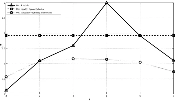
3.1 Optimal Schedules under Different Policies . . . 39
4.1 Optimal Solution of Single Service Queue Model . . . 58
5.1 Two-Coupled-Queue Model . . . 62
5.2 Direct & Indirect Delaysvs. IAT: Scenario 1 . . . 82
5.3 Direct & Indirect Delaysvs. IAT: Scenario 2 . . . 82
5.4 Direct & Indirect Delaysvs. IAT: Scenario 3 . . . 83
5.5 Direct & Indirect Delaysvs. IAT: Scenario 4 . . . 83
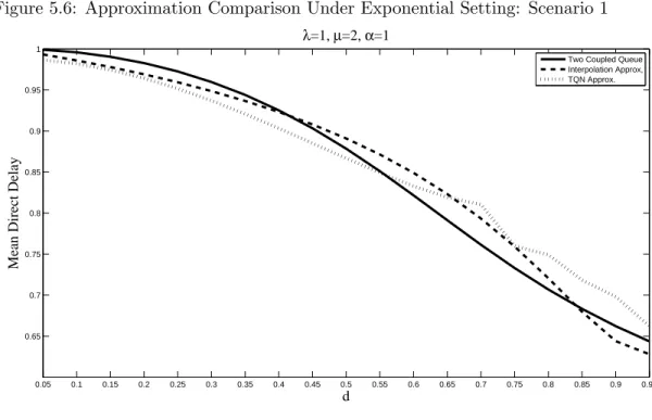
5.6 Approximation Comparison Under Exponential Setting: Scenario 1 . . . 84
5.7 Approximation Comparison Under Exponential Setting: Scenario 2 . . . 85
5.8 Approximation Comparison Under Exponential Setting: Scenario 3 . . . 85
5.9 Approximation Comparison Under Exponential Setting: Scenario 4 . . . 86
5.10 Performance Comparison Under Lognormal Setting: Scenarios 1–4 . . . 87
5.11 Performance Comparison Under Lognormal Setting: Scenarios 5–8 . . . 87
List of Tables
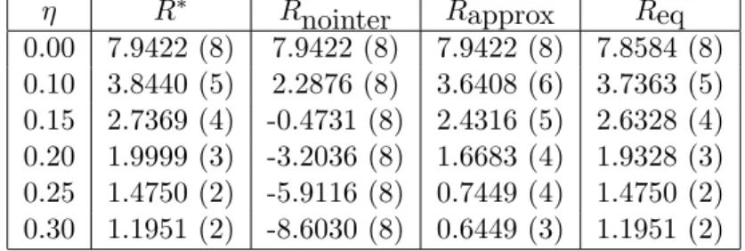
3.1 Numerical Results for Scenario 1 - Numbers in parentheses indicate N∗, the
optimal number of appointments to be scheduled in each setting . . . 37
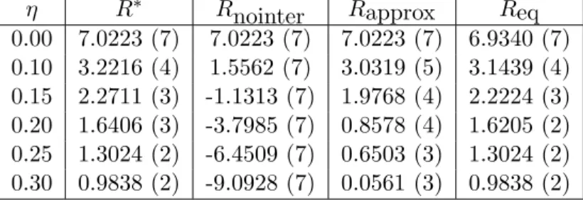
3.2 Numerical Results for Scenario 2 - Numbers in parentheses indicate N∗, the
optimal number of appointments to be scheduled in each setting . . . 38
3.3 Numerical Results for Scenario 3 - Numbers in parentheses indicate N∗, the
optimal number of appointments to be scheduled in each setting . . . 38
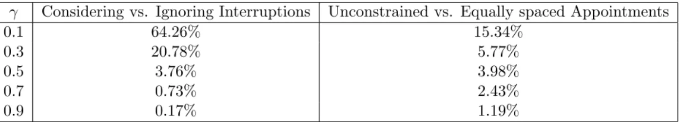
3.4 Benefits of Considering Interruptions and Allowing Flexible Appointment Times
under Scenario 1 . . . 41
3.5 Benefits of Considering Interruptions and Allowing Flexible Appointment Times
under Scenario 2 . . . 41
Chapter 1
Introduction
Appointment systems mainly work to regulate customer demand for various services with
limited capacity. They help balance the basic trade-off between service utilization and
cus-tomer waiting (delays) by reducing the variability in the cuscus-tomer arrival process to service
systems. However, it is not possible to eliminate the variability completely. Customers may
arrive earlier or later than their scheduled appointment times, or they may simply not show
up at all. It may take longer than expected to serve a particular customer, or the service
can be interrupted for various reasons, including arrivals of emergency customers who need
to be attended to right away. Some of these factors have been investigated within the large
and growing body of work on appointment scheduling, but some of them have been barely
studied by prior work. The objective of this dissertation is to develop a better understanding
of these issues that are commonly observed in practice but are not investigated sufficiently in
the academic literature so far.
1.1
Appointment Scheduling in the Presence of Service
Inter-ruptions
Service interruptions are prevalent in a wide class of appointment-based service systems. The
primary motivation comes from applications in healthcare, where service interruptions are
mostly caused by emergency patients who need immediate attention. For example,
e.g., Kenny and Barrett (2005); Alderman (2011)). Many healthcare clinics of various
spe-cialties and dental offices warn their patients in advance that in case of emergencies, they
may experience longer waiting times (see, e.g., http://www.nwh.org/clinical-centers/
spine-center/patient-faq, http://www.northfultonpediatrics.com/policies, http:
//princetonpediatricdentist.com/faqs). In fact, interruptions to scheduled
appoint-ments are not necessarily caused by patients in need of immediate attention. According
to Klassen and Yoogalingam (2008), such interruptions may include calls from other doctors
or pharmacists and problems that require dealing with the administrative staff. The
inter-rupted process can also be the service provided by a diagnostic machine. Typically, patients
make appointments for access to computerized tomography (CT) scans or magnetic
reso-nance imaging (MRI) machines at hospitals. However, frequently, emergency physicians find
it necessary to use these machines for emergency patients who cannot “afford” to wait. Such
patients, when sent for a diagnostic scan, get higher priority than and cause additional delays
for the regular patients who have scheduled appointments (see, e.g., Green et al. (2006)).
Recent studies suggest that the rate of such emergency use of these machines is quite high
and has been increasing significantly over the last years. For example, Korley et al. (2010)
conducted a national survey of patient visits to emergency departments within the United
States and found that the percentage of emergency department visits that required the use
of CT scan or MRI increased from 6% in 1998 to 15% in 2007. Broder and Warshauer (2006)
analyzed adult patient data from the emergency department of a university hospital. They
found that from 2000 to 2005, the adult emergency department volume increased by 13%;
head CT scans increased by 51%, cervical spine CTs by 463%, chest CTs by 226%, abdominal
CTs by 72%, and miscellaneous CTs by 132%. These numbers clearly show the significant
increase in the use of the CT scan at this hospital over a five-year period. The authors have
also observed that except for the abdominal CT, which seemed to level off over the last year of
the five-year period, the numbers of all types of CT scans have consistently increased at a rate
higher than that for the adult patient volume. Another study carried out at the emergency
department of the HealthAlliance Hospital in Leominster, Massachusetts, found that roughly
department and that these patients were given top priority for access to radiology services
with no delay ( Anderson et al. (2010)). The disruption of regularly scheduled appointments
by emergencies could be prevented if emergency departments had dedicated diagnostic
ma-chines. However, because it is prohibitively costly to have a dedicated diagnostic machine
for the exclusive use of emergency patients, this solution is not feasible for most hospitals.
Hence there is usually a strong incentive to keep diagnostic machines as highly utilized as
possible (see Green et al. (2006)). Therefore, these machines are typically shared by regular
patients, who schedule appointments in advance, and emergency patients, who come without
appointments and get higher priority.
Earlier work on appointment scheduling has provided many useful insights on how
ap-pointments should be scheduled over a given period of time when there are no interruptions
to the service process. However, it is not known whether and how explicit consideration of
in-terruptions (e.g., emergency cases) would change these earlier insights. One of the objectives
of this research is to investigate this question. For example, we know that when the service
times are independent and identically distributed, and there are no interruptions to the service
process, the optimal scheduling policy has a “dome” shape, meaning that the times between
consecutive appointments that are scheduled early or late in the day are small, whereas the
times between those scheduled midday are larger (see Hassin and Mendel (2008)). We also
know that requiring the time between any two consecutive appointments to be the same does
not degrade the policy performance significantly (see Stein and Cˆot´e (1994)). The question is
whether these observations are valid in the presence of interruptions as well. When there are
interruptions, does the optimal policy still have a dome shape, and does the optimal policy
under the restriction that appointments are scheduled at equally spaced intervals perform
suf-ficiently well? Perhaps there is no good reason to suspect that the answers to these questions
would be any different when emergency cases arrive with some fixed rate, but what if the rate
changes depending on the time of the day? For example, the rate of arrivals to emergency
departments is known to be time dependent, which means that the arrival rate of emergencies
to the diagnostic machines is also very likely to be time dependent. In such cases, one can see
make more sense to schedule fewer appointments around the times when the arrival rates of
emergency cases are higher.
1.2
Appointment Delay and Service Delay in An Appointment
System
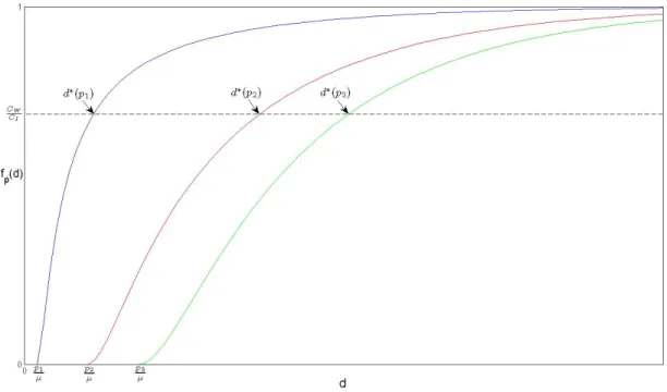
Customers encounter two types of access delays in an appointment system, namely
appoint-ment delay (indirect delay) and service delay (direct delay) (see Gupta and Denton (2008)).
Appointment delay is the difference between the time that a customer requests an
appoint-ment and the actual appointappoint-ment time scheduled for that customer. Service delay is the
difference between the time a customer arrives at the service facility (the appointment time
if he is punctual) and the time when he is actually served. The service providers prefer to
keep appointment intervals short in order to minimize the server idle time. However, short
appointment intervals tend to cause congestion in the waiting room, which results in long
direct waiting time. On the other hand, if appointments are scheduled sparsely, customers
may encounter long indirect delay. Gallucci et al. (2005) point out that the longer the
ap-pointment delay, the more likely that customers will cancel their apap-pointments or become
no-shows. Customer no-show behavior results in the waste of service resources while other
customers encounter long waits in getting appointments. For instance, the time slot assigned
to a customer who becomes a no-show may not be reassigned to another customer but may
be wasted. As a result, while long direct delay might lead to customer dissatisfaction about
the service, long appointment delays may not only cause dissatisfaction, but may also lead
to appointment cancellations, no-shows, or patients choosing to be served elsewhere, which
results in the loss of revenue for the practice (see Green and Savin (2008)).
Despite the significant impact that both direct and indirect delays have on the
perfor-mance of appointment systems, Gupta and Denton (2008) point out that the majority of the
literature on appointment scheduling has concentrated on the problem of balancing customer
direct delay and server utilization over a service session. The typical decision variables in
slot, the number of customers assigned to each slot, and so on (e.g., Mercer (1973), Stein
and Cˆot´e (1994), Wang (1997), and many others). Few papers take customer indirect waiting
into consideration (e.g., Green and Savin (2008) and Liu et al. (2010)). Clearly, however,
appointment scheduling should ideally take into account indirect and direct waiting times
si-multaneously (e.g., Creemers and Lambrecht (2009)) because both of them affect customers’
service experiences significantly. Thus, a portion of this thesis is devoted to the problem of
designing an efficient appointment system that aims to balance the utilization of expensive
service resources and the delays (both direct and indirect) encountered by customers.
The remainder of this thesis is organized as follows: Chapter 2 gives a review of the
related literature. In Chapter 3, we develop analytical methods for determining appointment
schedule in the presence of service interruptions, evaluate the importance of incorporating
service interruptions in the decision models, and identify the structural properties of the
optimal policies. Chapter 4 considers a simple version of the appointment system design
problem by assuming the pool of customers who request service is infinitely large. In Chapter
5, we carry out a steady-state analysis of an appointment system by taking account of both
direct and indirect delays. Finally, Chapter 6 point out several potential research directions
Chapter 2
Literature Review
The operations management literature on appointment scheduling is vast and rapidly
expand-ing. For an extensive review of this literature, as well as discussions on directions for future
research, we refer the reader to Cayirli and Veral (2003) and Gupta and Denton (2008). Here,
we only mention those papers that are either very closely related to the work in this thesis or
very recent.
2.1
Queueing Models of Appointment Systems
Gupta and Denton (2008) propose a useful classification scheme for appointment-scheduling
models depending on the type of waiting that is formulated. They define a patient’s direct
waiting time as the time the patient spends in the clinic on the day of his appointment and
indirect waiting timeas the time between the patient’s call for an appointment and the sched-uled appointment time. There is some relatively recent work on indirect waiting (see Gupta
and Wang (2008), Green and Savin (2008), Liu et al. (2010)), but the vast majority of the
papers focus on performance measures related to direct waiting. The following
appointment-scheduling literature is introduced based on the above categorization proposed by Gupta and
2.1.1 Direct Waiting
Starting from the pioneer work of Bailey (1952), appointment systems have been studied
extensively by using queueing models. When determining appointment times on a given day,
there are a number of objectives, including keeping the server (e.g, physician) busy, keeping
waiting times short, and avoiding or minimizing overtime. Papers that deal with direct
wait-ing time typically consider one or more of these objectives, in many cases by minimizwait-ing an
objective function that is a weighted sum of a subset of these various performance measures
(weighted by their relative “costs”) and/or adding them as constraints into the formulation.
For example, Jansson (1966) models such an appointment system as aD/M/1 queuing system
and obtains the optimal interarrival time. Fries and Marathe (1981) develop a dynamic
pro-gramming approach to obtain the optimal scheduling of finite number of patients into finite
number of appointment slots with equal length. A similar model is considered in Kaandorp
and Koole (2007) that accommodates the patient no-show behavior. A number of articles
study the appointment systems where the interarrival times are not necessarily equal.
Peg-den and Rosenshine (1990) determine the optimal schedule of a finite number of appointment
requests that minimizes the sum of customer direct waiting and server availability costs.
Has-sin and Mendel (2008) extend the model studied in Pegden and Rosenshine (1990) by taking
customer no-shows into consideration. Wang (1999) investigates the problem of scheduling
a finite number of patients who require exponential amount of service time with different
rates. He obtains the optimal schedule that determines the order in which customers are
served as well as their appointment times. Denton and Gupta (2003) develop a two-stage
stochastic linear program to solve the appointment scheduling problem in which customers
arrive punctually with random service demands. All the above research work assumes that
the relative “costs” of the performance measures are known and the objective is to find the
optimal appointment schedule. Robinson and Chen (2011), however, do the opposite by
ob-taining an estimation of the relative costs based on the assumption that the appointment
system is already operated optimally. For more work in this stream of research, see Pegden
(2008).
Multi-priority appointment scheduling has also been studied by a number of research
arti-cles. Green et al. (2006) and Patrick et al. (2008) both formulate the appointment scheduling
of outpatients and inpatients who share the use of a diagnostic medical facility as a discrete
Markov decision process. Gupta and Denton (2008) develop a dynamic programming model
for scheduling regular and same-day patients by taking patient preferences into consideration.
Luo et al. (2012) investigate the appointment scheduling problem in which scheduled service
can be preemptively interrupted by emergencies.
Mercer (1973), Doi et al. (1997), and Jouini and Benjaafar (2012) study the
appointment-driven queueing system by accommodating customer tardiness and no-show behavior.
Over-booking is also a commonly used strategy when scheduling appointments with no-shows
and/or cancellations. LaGanga and Lawrence (2007), Muthuraman and Lawley (2008),
Chakraborty et al. (2010), and Robinson and Chen (2010) develop the appointment scheduling
policies that use overbooking to compensate for patient no-shows with different assumptions
on service demand and service time distribution.
2.1.2 Indirect Waiting
As mentioned in the beginning of this chapter, the majority of the appointment-scheduling
literature has focused on performance measures related to direct waiting. The importance
of consideration of indirect delay has drawn more attention of recent researchers. Gallucci
et al. (2005) point out that the longer the appointment delay, the higher the chances that a
customer will cancel his appointment or become a no-show. Green and Savin (2008) formulate
an appointment scheduling system as anM/D/1/K queue in which the no-show probability
is assumed to be an explicit function of the appointment backlog. Creemers and Lambrecht
(2009) develop a formulation that considers indirect and direct waiting times simultaneously.
Liu et al. (2010) propose heuristic dynamic policies for scheduling patient appointments by
taking into account the fact that patients may cancel or not show up for their appointments
2.2
Appointment Scheduling in the Presence of Interruptions
Limited work on interruptions has appeared within the context of appointment scheduling.
Three papers, Pegden and Rosenshine (1990), Stein and Cˆot´e (1994), and Hassin and Mendel
(2008), are special case of our work discussed in Chapter 3. Specifically, Pegden and
Rosen-shine (1990) obtain a closed-form solution for the optimal schedule for the case where there
are only two appointments; they develop a method to compute the optimal schedule for the
general case with more than two appointments. What is mainly different in the model of
Peg-den and Rosenshine (1990) (with respect to our formulation) is that all customers show up
for their appointments and the service process never gets interrupted. Stein and Cˆot´e (1994)
mainly build on Pegden and Rosenshine (1990) and study the effect of requiring equally
spaced appointment times. On the other hand, Hassin and Mendel (2008) generalize the
model of Pegden and Rosenshine (1990) by allowing no-shows. They carry out a numerical
study and generate insights on the structure of the optimal appointment policy, the
impor-tance of modeling no-shows, the effects of no-shows on the optimal policy and its performance,
and the “cost” of forcing equidistant appointments. We generalize the model of Hassin and
Mendel (2008) by allowing the service of scheduled patients to possibly be interrupted. In
Chapter 3, We mainly investigate the importance of modeling interruptions and how their
existence changes the main insights obtained earlier in the literature, mostly in these three
papers.
In addition, we are aware of three other papers that share our primary motivation, as
they also deal with service interruptions at outpatient clinics and diagnostic machines.
How-ever, these papers use completely different analytical techniques and/or structurally different
formulations. In particular, Klassen and Yoogalingam (2008) study nonemergency physician
interruptions in an outpatient clinic using simulation optimization. Fiems et al. (2012) develop
a queueing model and carry out steady-state analysis to investigate the impact of emergency
requests on the waiting time of regularly scheduled patients in the radiology department.
On the other hand, Vasanawala and Desser (2005) develop a simple mathematical model to
requests.
There are also papers (many from the traditional job-scheduling and queueing literature)
that analyze models in which the service might get interrupted because of a server failure or
vacation. However, with one exception, which we discuss below, these papers make
assump-tions that do not fit well with the appointment-scheduling problem. For example, Federgruen
and Green (1986), Takine and Sengupta (1997), and Gray et al. (2000) all consider queueing
models in which the server can go on and off, but they assume that customers arrive according
to some stationary process (e.g., Poisson) and carry out steady-state analysis. Glazebrook
(1984), Adiri et al. (1989), and Birge et al. (1990), on the other hand, assume that all jobs are
available to be processed at the beginning of the service session and the decision to be made
is the order in which these jobs will be processed. One exception from the job-scheduling
literature is the work of Wang (1994), which develops an algorithm that determines the
op-timal release times of a finite number of jobs to an unreliable machine. His model is in fact
almost the same as ours with one difference being our consideration of the possibility of
no-shows. However, there is one important error in the analysis of Wang (1994) that affects the
resulting expressions and methods significantly. The error is related to the author’s implicit
independence assumption in the derivation of an equation when, in fact, there is dependence.
Chapter 3
Appointment Scheduling Under Service
Interruptions
3.1
Introduction
We consider an appointment-based service system (e.g., an outpatient clinic) for which
ap-pointments need to be scheduled before the service session starts. Patients with scheduled
appointments may or may not show up for their appointments. The service of scheduled
patients can be interrupted by emergency requests that have a higher priority. We develop
a framework that can be utilized in determining the optimal appointment policies under
dif-ferent assumptions regarding rewards, costs, and decision variables. We specifically consider
two different formulations, both of which aim to balance the trade-off between the patient
waiting times and server utilization.
Our proposed appointment-scheduling model differs from prior models mainly in that the
service of regularly scheduled patients can be temporarily suspended because of
interrup-tions. Our model can be seen as a generalization of the model of Hassin and Mendel (2008),
who implicitly assumed that there are no interruptions. We assume that interruptions
oc-cur according to a Poisson process, but we allow the interruption rate to change with time.
This is one of the important features of our formulation, as it fits nicely with our
motivat-ing applications. The complexity of our formulation makes it very difficult if not impossible
simpler case, where there are no interruptions, Hassin and Mendel (2008) resort to numerical
analysis to generate insights on the problem. In fact, even a simple computation of the
objec-tive function for a given appointment schedule is a significant challenge in our optimization
problem; therefore, the core of our analysis is devoted to the question of how this computation
can be done. In particular, the computation requires the solution of a system of differential
equations, which is not readily available. However, we provide two different methods, either
of which can be used to find a solution and thus compute the objective function. After
de-veloping these solution methods, we use them for a numerical study to quantify the potential
benefits of incorporating the interruption process into the formulation, we then investigate
how explicit consideration of interruptions influences the key insights on optimal appointment
scheduling. We find that ignoring interruptions when they are in fact prevalent can result in
appointment schedules that demonstrate significantly worse performances. We also find that
policies that require equally spaced appointments perform reasonably well when the
interrup-tion rate is constant. However, their performance worsens significantly when the interrupinterrup-tion
rate is time dependent.
The remainder of this chapter is organized as follows: In Sections 3.2 and 3.3, we introduce
the formulation of appointment scheduling in the presence of preemptive service interruptions.
In Section 3.4, we develop the two methods that can be used to compute the objective function.
Section 3.5 demonstrates how the method for computing the objective function can also be
used in computing the expected patient waiting time and server overtime. In Section 3.6
we show how our formulation can be generalized to allow the interruption time to have a
phase-type distribution. In Section 3.7, we introduce the model with nonpreemptive service
interruptions. Section 3.8 provides our numerical results. Section 3.9 explains an error we
find in the work of Wang (1994) that develops a similar model as ours in the manufacturing
3.2
Model Description
The methodology we use in this chapter can be used in a variety of formulations that consider
the scheduling of a finite number of appointments over a finite or infinite horizon. We consider
two such formulations, one of which has received significant attention in the literature, but
with the restriction that there are no service interruptions. To keep the presentation simple,
we introduce the models assuming that interruptions occur according to a homogeneous
Pois-son process. In Section 3.8, we explain how our analysis can easily be extended to the case
where interruptions occur according to a nonhomogeneous Poisson process, and we provide
numerical results under that generalization.
3.2.1 Model I: Restricted scheduling horizon
Suppose that there is a predetermined scheduling horizon [0, T] where T < ∞. At time
zero, we need to decide N, the number of appointments to be scheduled over this time
interval, as well as the times for these N appointments. We define dk as the appointment
time scheduled for the kth patient, k = 1,2, . . . , N. The vector d = (d1, d2, . . . , dN), where
0 ≤d1 ≤ d2 ≤ . . .≤ dN ≤ T, is called a schedule for these N patients. Scheduled patients
either show up punctually at their appointment times with probability p or become
no-shows in an independent manner. Patients who show up are served on a come
first-served basis. The service times for patients are assumed to be independent and identically
distributed according to an exponential distribution with mean 1/µ. However, services can
be interrupted by certain events, which we assume to occur according to a Poisson process
with rateη. Once the server is interrupted, it stays in that stage for an amount of time that is
exponentially distributed with rateθ, and during that time any new interruptions are assumed
to have no effect. In Section 3.6, we show how the exponential distribution assumption on
the interruption times can be relaxed by allowing them to have a phase-type distribution,
which also makes it possible to model more explicit connections between interruption events
and the interruption durations (e.g., explicit modeling of emergency patients who queue up).
patient is suspended immediately in the presence of interruptions and resumes with no loss
of work when the server becomes available again.
It might be helpful to think of the whole service horizon as a sequence of “on” and
“off” periods. During the “on” periods, the server is available to work on regularly scheduled
patients. During the “off” periods, the server is not available and is engaged in other activities,
such as attending to emergency patients. At time zero, the server is available for serving
scheduled patients; that is, the service session starts with an “on” period. An interruption
ends this “on” period and starts an “off” period, during which no scheduled patients can be
served. Once this period is over, the server becomes available for scheduled patients again and
another “on” period starts. The server status alternates between these “on” and “off” states
until the services of all the scheduled patients who show up are completed. Even though all
appointments need to be scheduled some time between 0 and T, it is possible that some of
the scheduled patients will be served after timeT. Note that, even after time T, services of
the regular patients can still be interrupted. However, if all the scheduled patients who show
up are served by T, the server is turned off and no more interruptions occur.
The system incurs the waiting cost from scheduled patients (the waiting time of a
sched-uled patient is the total time the patient spends in the system minus the time in service) and
the server overtime cost if the service completion time of all the patients who show up is later
thanT. We use cw to denote the patient waiting cost per unit of time andcl to denote the
server overtime cost per unit of time beyond T. In addition, the system earns a reward r
from each scheduled patient who receives service. The objective is to find the optimal policy
(N∗,d∗) to maximize Π(N,d), the total expected net profit, which is the reward from serving
scheduled patients minus the patient waiting and the server overtime cost.
3.2.2 Model II: Unrestricted scheduling horizon
Model II makes the same assumptions as Model I regarding patients’ service times, no-show
behavior, and service interruption process, but differs from Model I in a few important aspects.
Most importantly, N, the total number of appointments to be scheduled, is not a decision
T = ∞). In other words, the number of appointments to be scheduled is given and the
decision to be made at time zero is at what time to schedule these appointments. The
system keeps operating until the appointment time assigned to theNth patient or the service
completion time of the last patient who shows up, whichever is later. We consider two types
of cost: cw, as defined in Model I, and cs, the cost of operating the system per unit of time
(service availability cost). The objective is to find the optimal scheduled∗for theseN patients
to minimize the total expected cost. Note that this model reduces to the model of Hassin
and Mendel (2008) if we assume that there are no service interruptions and the server is
available at all times; it reduces to the model of Pegden and Rosenshine (1990) if we further
assume that (in addition to the no interruption assumption) all patients show up for their
appointments.
3.3
Complete Description of the Optimization Problem
In this section, we provide a more complete description of the optimization problem for Model
I. It is important to note that the treatment of the optimization problem in Model II is similar,
with some minor differences; therefore, we skip it for brevity.
3.3.1 Formal Statement of the Optimization Problem
Our optimization problem can briefly be stated as follows:
max
N,d Π(N,d)
s.t. 0≤d1 ≤d2≤. . .≤dN ≤T
where Π(N,d) is the total expected net profit.
An analytical characterization of the optimal policy does not appear to be possible because
of the complexity of the problem. Therefore, a more realistic goal, which we pursue in this
chapter, is to develop a numerical solution method. In fact, even the computation of the
expression. We can, however, obtain Π(N,d) by solving a system of differential equations, as we demonstrate in the following.
3.3.2 Effective Service Time
Even though the time it takes to serve a scheduled patient has an exponential distribution,
the time between the start of a given patient’s service and its end, called theeffective service
time, is not exponentially distributed because of the possibility of interruptions. Let X be
the effective service time of a scheduled patient who shows up, and let G(t) = P{X ≤ t}.
Recall that η is the Poisson arrival rate of interruptions, 1/µ is the mean service time, and
1/θ is the mean interruption time. One can show that (see the proof of Proposition 3.6.1 in
Appendix A of the online supplement)
G(t) = (1−β)(1−e−at) +β(1−e−bt), (3.1)
whereβ = µb−−aa, and
a= 1 2
h
η+µ+θ+p(η+µ+θ)2−4θµi>0, (3.2)
b= 1 2 h
η+µ+θ−p(η+µ+θ)2−4θµi>0. (3.3)
Hence,X is a mixture of two exponential distributions and its mean is given by
E(X) = Z ∞
0
(1−G(t)) dt= η+θ
θµ . (3.4)
3.3.3 Recursive Expression for the Objective Function
In this section, we derive the system of differential equations, which needs to be solved to
evaluate the objective function Π(N,d). To that end, first denote the server state by 0 if it
is available for scheduled patients and by 1 if not. Let d0 = 0 and dN+1 = T. Also define
the net profit function associated with each appointment interval [dk, dk+1), k= 0,1, . . . , N
the system over [dk+1−t,∞) if at timedk+1−tthere are nscheduled patients in the system
and the server is in state i, where n= 0,1, . . . , k, andi= 0,1. We assume that the server is
available for scheduled patients at time zero, and thus R00,0(d1) is the net profit the system
earns over [0,∞). Consequently, we have Π(N,d) =R00,0(d1).
To obtain R0
0,0(d1) (or Π(N,d)), we first need to characterize the expected net profit
functionRkn,i(t) for each k= 0,1, . . . , N and for t∈(0, dk+1−dk], that is, between any two
consecutive appointment times, in the interior of the appointment interval. In addition, we
need to establish how Rkn,i(t) for different values of k, n, andi are related. To do this, for
each k= 0,1, . . . , N,n= 0,1, . . . , k, and t ∈(0, dk+1−dk], denote Rkn(t) =
Rkn,0(t)
Rkn,1(t)
, and
dRk
n(t)
dt =
dRk
n,0(t)
dt
dRk
n,1(t)
dt
. Also let A =
µ 0 0 0 , B =
−(η+µ) η θ −θ
, E =
−η η θ −θ
, and
Cw =
cw cw
. We can prove the following theorem:
Theorem 3.3.1. For each k = 0,1, . . . , N, the vector of the net profit functions Rkn(t),
0< t≤dk+1−dk, satisfies the following differential equations:
dRk0(t)
dt =ER
k
0(t), (3.5)
dRkn(t)
dt =−
n−1 0
0 n
Cw+AR
k
n−1(t) +BRkn(t), n= 1, . . . , k, (3.6)
with boundary conditions
R0N,0(0+) =RN0,1(0+) = 0, (3.7)
RNn,0(0+) =−clnE(X)−cw
n(n+ 1)
2 E(X)−
n µ
, n= 1, . . . , N, (3.8)
RNn,1(0+) =−cl(
1
θ +nE(X))−cw
n θ +
n(n+ 1)
2 E(X)−
n µ
, n= 1, . . . , N, (3.9)
Rn,ik (0+) =p(r+Rnk+1+1,i(dk+2−dk+1))
Proof. Depending on the server state and the number of scheduled patients in the system,
the following events might occur during (dk+1−(t+h), dk+1−t) (Kulkarni, 1995, p. 206):
If no patient is in the system and the server is available at dk+1 −(t+h), then at
dk+1−t the server becomes unavailable with probability ηh+o(h), or stays available
with probability 1−ηh+o(h).
If there is at least one scheduled patient in the system and the server is available at
dk+1−(t+h), then atdk+1−tthe number of scheduled patients in the system is reduced
by 1 with probability µh+o(h), or the server becomes unavailable with probability
ηh+o(h), or both the number of scheduled patients in the system and the server state
remain unchanged with probability 1−µh−ηh+o(h).
If the server is unavailable atdk+1−(t+h), then at dk+1−t, the number of patients in
the system does not change, and the server becomes available with probabilityθh+o(h),
or stays unavailable with probability 1−θh+o(h).
Then, fork= 0,1, . . . , N, we have
Rk0,0(t+h) = (ηh+o(h))Rk0,1(t) + (1−ηh+o(h))Rk0,0(t),
Rk0,1(t+h) = (θh+o(h))Rk0,0(t) + (1−θh+o(h))Rk0,1(t),
Rkn,0(t+h) =−(n−1)cwh+ (µh+o(h))Rkn−1,0(t) + (ηh+o(h))Rkn,1(t) + [1−(η+µ)h+o(h)]Rkn,0(t),
Lettingh→0, after some algebra, we have the following:
dR0k,0(t)
dt =−ηR
k
0,0(t) +ηRk0,1(t),
dR0k,1(t)
dt =θR
k
0,0(t)−θR0k,1(t),
dRkn,0(t)
dt =−(n−1)cw+µR
k
n−1,0(t) +ηRkn,1(t)−(η+µ)Rkn,0(t),
dRk n,1(t)
dt =−ncw+θR
k
n,0(t)−θRkn,1(t), n= 1, . . . , k.
(3.5) and (3.6) are then obtained by writing the above differential equations in the matrix
form.
To obtain the boundary conditions, we start with the net profit that would be incurred
afterT. When there are n≥1 scheduled patients in the system just prior toT and the server
is available, the expected amount of time the system will continue to be operated isE(nX),
which is also equal to the expected server overtime. And the expected total waiting time
these nscheduled patients will spend in the system is
E[nX + (n−1)X+· · ·+X]−n
µ =
n(n+ 1)
2 E(X)−
n µ.
If the server is unavailable, the expected overtime and the expected waiting time for each
scheduled patient in the system are increased by 1/θ.
We also need to state the boundary conditions across appointment intervals. Specifically,
at timedk,k= 1,2, . . . , N, if the kth scheduled patient shows up, the system earns a reward
r, the total number of patients in the system is increased by 1, and the number of pending
appointments is decreased by 1. Otherwise, the system earns no reward, the total number
of patients in the system remains unchanged, and the number of pending appointments is
Theorem 3.3.1 states the differential equations that the functions Rkn(·) need to satisfy, but the solution to these equations is not directly available. In Section 3.4, we describe how
to solve them.
3.4
Two Methods for Computing the Objective Function
In this section, we propose two methods, the method of Laplace transform (LT) and the
method of integrating factor, both of which can be used to evaluate the objective function,
Π(N,d), for givenN and d.
3.4.1 Method I: Using Laplace Transforms
For eachk= 0,1, . . . , N,Rkn(t) is defined on t∈(0, dk+1−dk]. To apply the method of LT,
the domain of Rkn(t) is extended to be t ∈ (0,∞). After Rnk(t) is obtained, we only need
its values on t ∈ (0, dk+1−dk]. Let ˜Rkn(s) denote the LT of Rkn(·) for k = 0,1, . . . , N and
n = 0,1, . . . , k. Then we can show that ˜Rkn(s) can be obtained recursively as stated in the following theorem:
Theorem 3.4.1. For each k= 0,1, . . . , N, we have
˜
Rk0(s) = (sI−E)−1Rk0(0+), (3.11)
˜
Rkn(s) =(sI−B)−1An(sI−E)−1Rk0(0+)+
n−1 X
j=0
(sI−B)−1Aj(sI−B)−1
−
n−1−j 0
0 n−j
Cw
s +R
k n−j(0+)
, n= 1, . . . , k,
(3.12)
where Rk0(0+) and Rkn−j(0+),j = 0, . . . , n−1, can be obtained using the boundary conditions
(3.7)–(3.10).
Proof. For eachk= 0,1, . . . , N, taking the LT of (3.5) and (3.6), we have
sR˜kn(s)−Rkn(0+) =−
n−1 0
0 n
Cw
s +AR˜
k
n−1(s) +BR˜kn(s), n= 1, . . . , k.
Thus,
˜
Rk0(s) = (sI−E)−1R0k(0+),
˜
Rnk(s) = [(sI−B)−1A] ˜Rkn−1(s) + (sI−B)−1[−
n−1 0
0 n
Cw
s +R
k n(0+)]
= [(sI−B)−1A]n(sI−E)−1Rk0(0+)
+
n−1 X
j=0
{[(sI−B)−1A]j(sI−B)−1[−
n−1−j 0
0 n−j
Cw
s +R
k
n−j(0+)]}.
For a given schedule d = (d1, d2, . . . , dN), Theorem 3.4.1 suggests a recursive procedure
that can be used to obtain the LT ˜Rkn(s) for each k= 0,1, . . . , N and n= 0,1, . . . , k, which
can then be inverted to obtain Rkn(t). In particular, R00,0(t) is equal to Π(N,d) for t = d1.
The following algorithm is a detailed description of this recursive procedure:
Algorithm 1
Step 1. Initialize: Setk=N. ComputeE(X), the expected length of the effective service
time and use (3.8) and (3.9) to evaluateRNn(0+) for n= 0,1, . . . , N.
Step 2. Apply (3.11), (3.12), and the boundary constraint (3.10) to compute ˜Rk
n(s), the
LT of Rkn(t), forn= 0,1, . . . , k.
Step 3. For each n = 0,1, . . . , k, invert ˜Rnk(s) to obtain Rkn(t) and evaluate its value at
t=dk+1−dk, which will be used in Step 2 of the next iteration.
Step 4. Ifk >0, set k=k−1 and go to Step 2. Otherwise, stop. The objective function
3.4.2 Inverting R˜kn(s)
In Step 3 of the above algorithm, we need to invert ˜Rkn(s) fork= 0,1, . . . , N andn= 0, . . . , k
in order to obtain Rkn(t). Since all the terms appearing in (3.11) and (3.12) are rational
functions ofs, the inversion can be done by the method of partial fraction decomposition (see
Horowitz (1971)). We shall use the term
[(sI−B)−1A]n(sI−E)−1
s , n≥1
that appears in (3.12) as an example to illustrate how this method works. It is easy to verify
that, forn≥1,
[(sI−B)−1A]n(sI−E)−1
s =
1
(s+a)n(s+b)ns2(s+η+θ)
(s+θ)n+1µn η(s+θ)nµn θ(s+θ)nµn ηθ(s+θ)n−1µn
.
(Recall thats2+ (η+µ+θ)s+µθ= (s+a)(s+b).)
Applying the partial fraction decomposition to the upper-right element, it takes the
fol-lowing form:
η(s+θ)nµn
(s+a)n(s+b)ns2(s+η+θ) =ηµ
n[x
s + y s2 +
z s+η+θ +
n
X
j=1
ej
(s+a)j + n
X
j=1
fj
(s+b)j],
where
x= ∂[
(s+θ)n
(s+a)n(s+b)n(s+η+θ)]
∂s |s=0, y= (s+θ)
n
(s+a)n(s+b)n(s+η+θ) |s=0,
z= (s+θ)
n
(s+a)n(s+b)ns2 |s=−(η+θ),
ej =
∂n−j[(s+b)(nss+2(θs)n+η+θ)]
∂sn−j |s=−a,
fj =
∂n−j[ (s+θ)n
(s+a)ns2(s+η+θ)]
To compute ej, j = 1,2, . . . , n, we need to find the mth derivative of (s+θ)
n
(s+b)ns2(s+η+θ) for
m= 0,1, . . . , n−1. This can be done by using the following technique: letg1(s) = (s+θ)n,
g2(s) = 1/(s+b)n,g3(s) = 1/s2, and g4(s) = 1/(s+η+θ). Then we have
∂m[ (s+θ)n
(s+b)ns2(s+η+θ)]
∂sm =
∂m(g1(s)g2(s)g3(s)g4(s))
∂sm
= X
m1+m2+m3+m4=m
m m1, m2, m3, m4
g(m1)
1 (s)g
(m2)
2 (s)g
(m3)
3 (s)g
(m4)
4 (s)
= X
m1+m2+m3+m4=m
m!
m1!m2!m3!m4!
g1(m1)(s)g2(m2)(s)g3(m3)(s)g4(m4)(s),
wheremi is a non-negative integer andg
(mi)
i (s) is themith derivative ofgi(s) with respect to
s, i= 1,2,3,4. Note that gi(s), i= 1,2,3,4 are simple functions. Thus the mith derivative
of gi(s) can be obtained easily. The coefficients fj, j = 1,2, . . . , n, can be obtained in the
same way.
The partial fraction decomposition of the other terms appeared in (3.11) and (3.12) can
be obtained similarly. As a result, ˜Rk
n,i(s) can be written as a linear sum of fractions, each of
which is in one of the following forms:
1
s,
1
s2, 1
s+η+θ,
1 (s+a)j,
1
(s+b)j, j= 1, . . . , n.
Hence by inverting ˜Rkn,i(s), we are able to obtain Rkn,i(t) as a linear sum of terms, each of
which is in one of the following forms:
1, t, e−(η+θ)t, t
j−1e−at
(j−1)!,
tj−1e−bt
(j−1)!, j = 1, . . . , n.
3.4.3 Method II: Using an Integrating Factor
An alternative and more direct way of determining the solution to the system of differential
equations given in Theorem 3.3.1 is to use the method of integrating factor. According to
this method, we multiply both sides of (3.6) by e−Bt, the “integrating factor”, and solve the
to the following theorem, which suggests a recursive procedure that can be used to determine
Rkn(t),k= 0,1, . . . , N andn= 0, . . . , k.
Theorem 3.4.2. Let
H=
−a+θ θ
η θ
1 b−θθ
, J =
b−θ θ
−η θ
−1 −aθ+θ
, and L= θ η θ η ,
where aandbare given by (3.2)and (3.3), respectively. For eachk= 0,1, . . . , N, and η >0,
Rkn(t) =Dkn(t) +znk, n= 0,1, . . . , k.
where zkn and Dnk(t) are given as follows:
z0k= [0,0]0, zkn=B−1(
n−1 0
0 n
Cw−Az
k
n−1), n= 1,2, . . . , k,
Dk0(t) =u00,k+v00,ke−(η+θ)t+m00,k,0e−at+q00,,k0e−bt, Dnk(t) =
n
X
j=−n
un,kj ej(a−b)t+
n
X
j=−n
vjn,ke[−(η+θ)+j(a−b)]t
+
n−1 X
j=0
n−1−j
X
i=0
mn,ki,j tie−[a+j(a−b)]t+
n−1 X
j=0
n−1−j
X
i=0
qi,jn,ktie−[b+j(b−a)]t, n= 1,2, . . . , k.
In the above equations, m00,k,0 = q00,,k0 = [0,0]0, u00,k = LR0,k(0+)
η+θ , v
0,k
0 =
−ER0,k(0+)
η+θ , and u n,k j ,
vn,kj , mn,ki,j , qi,jn,k, n= 1, . . . , k, can be obtained recursively, as described in Appendix A of the online supplement.
Proof. For eachk= 0,1, . . . , N, defineDk0(t) =eEtRk0(0+), andDnk(t) =eBt[Rt
0e
−BsADk
n−1(s)ds+
Rkn(0+)−znk], n= 1, . . . , k. From Theorem 1, it is easy to verify that Rk0(t) = eEtRk0(0+) =
D0k(t) +zk0. Let ¯Rnk(t) =e−BtRkn(t) and take the derivative on both sides, we then have
d ¯Rnk(t)
dt =e
−Bt[ARk
n−1(t)−
n−1 0
0 n
Cw] =e
−Bt[ADk
n−1(t) +Aznk−1−
n−1 0
0 n
Note that the induction Rkn−1(t) = Dnk−1(t) +znk−1 is used in the above derivation. Now integrating both sides of the above equation, we have
¯
Rkn(t) = Z t
0
e−BsADkn−1(s)ds+Rkn(0+) + (e
−Bt−I)B−1(
n−1 0
0 n
Cw−Az
k n−1),
Rkn(t) =eBt[ Z t
0
e−BsADnk−1(s)ds+Rkn(0+)−znk] +zkn=Dkn(t) +znk.
To obtain the explicit recursive expression of Dnk(t), we expand eBt, e−Bt, and eEt in the
matrix form. First, we can write matricesB and E as follows:
B= θ
b−a
−a+θ θ
−b+θ θ 1 1
−a 0
0 −b
1 b−θθ
−1 −aθ+θ
,
E= 1
η+θ
1 η
1 −θ
0 0
0 −(η+θ)
θ η
1 −1
.
Hence,
eBt= θ
b−a
−a+θ θ
−b+θ θ 1 1
e−at 0
0 e−bt
1 b−θθ
−1 −aθ+θ
=
θ b−a(He
−at+J e−bt),
e−Bt= θ
b−a
−a+θ θ
−b+θ θ 1 1
eat 0
0 ebt
1 b−θθ
−1 −aθ+θ
=
θ b−a(He
at+J ebt),
eEt= 1
η+θ
1 η
1 −θ
0 0
0 e−(η+θ)
θ η
1 −1
=
1
η+θ(L−Ee
−(η+θ)t).
Having the above expansions, we can further write
D0k(t) =eEtRk0(0+) = (L−Ee−(η+θ)t)R
k
0(0+)
η+θ , Dnk(t) = θ
b−a(He
−at+J e−bt)(Rk
n(0+)−zkn)
+ ( θ
b−a)
2(He−at+J e−bt)
Z t 0
Now fork= 0,1, . . . , N, and n= 1, . . . , k, define
m00,k,0 =q00,,k0 = [0,0]0, u00,k = LR
k
0(0+)
η+θ , v
0,k
0 =
−ERk0(0+)
η+θ , un,kj = ( θ
b−a)
2[H2A u
n−1,k j
a+j(a−b)+J
2A u
n−1,k j
b+j(a−b)], j=−n, . . . , n,
vjn,k= ( θ
b−a)
2[H2A v
n−1,k j
a+j(a−b)−(η+θ) +J
2A v
n−1,k j
b+j(a−b)−(η+θ)], j=−n, . . . , n,
mn,k0,0 = θ
b−aH(R
k
n(0+)−znk) + (
θ b−a)
2{H2A[
n−2 X
j=1
n−2−j
X
i=0
i!
[j(a−b)]i+1m
n−1,k i,j
−
n−1 X
j=−n+1
unj−1,k a+j(a−b) −
n−1 X
j=−n+1
vjn−1,k
−η−θ+a+j(a−b)
+
n−2 X
j=0
n−2−j
X
i=0
i!
[(j+ 1)(b−a)]i+1q
n−1,k i,j ]−J
2A
n−2 X
i=0
i!(a−b)−(i+1)mni,−01,k},
mn,ki,0 = ( θ
b−a)
2[H2Am
n−1,k i−1,0
i −J
2A
n−2 X
s=i
s!
i!(a−b)
i−s−1mn−1,k
s,0 ], i= 1,2, . . . , n−1,
mn,ki,j = ( θ
b−a)
2{−H2A
n−2−j
X
s=i
s!
i![j(a−b)]
i−s−1mn−1,k s,j
−J2A
n−2−j
X
s=i
s!
i![(j+ 1)(a−b)]
i−s−1mn−1,k
s,j }, j= 1, . . . , n−1, i= 0, . . . , n−1−j,
q0n,k,0 = θ
b−aJ(R
k
n(0+)−zkn) + (
θ b−a)
2{J2A[
n−2 X
j=1
n−2−j
X
i=0
i! [j(b−a)]i+1q
n−1,k i,j
−
n−1 X
j=−n+1
unj−1,k b+j(b−a) −
n−1 X
j=−n+1
vjn−1,k
−η−θ+b+j(b−a)
+
n−2 X
j=0
n−2−j
X
i=0
i!
[(j+ 1)(a−b)]i+1m
n−1,k
i,j ]−H2A n−2 X
i=0
i!(b−a)−(i+1)qi,n0−1,k},
qi,n,k0 = ( θ
b−a)
2[J2Aq
n−1,k i−1,0
i −H
2A
n−2 X
s=i
s!
i!(b−a)
i−s−1qn−1,k
s,0 ], i= 1,2, . . . , n−1,
qi,jn,k= ( θ
b−a)
2{−J2A
n−2−j
X
s=i
s!
i![j(b−a)]
i−s−1qn−1,k s,j
−H2A
n−2−j
X
s=i
s!
i![(j+ 1)(b−a)]
i−s−1qn−1,k
Note that in the above recursions, un,kj and vn,kj , n = 0,1, . . . , k exist only if −n ≤ j ≤ n.
Otherwise, their values are defined to be 0. In the recursions formn,ki,j andqi,jn,k, if a sum interval
does not exist, the corresponding sum is defined to be 0. Using the fact thatHJ =J H = 0,
it can be shown that (the detailed algebra is omitted for brevity)
D0k(t) =u00,k+v00,ke−(η+θ)t+m00,k,0e−at+q00,k,0e−bt,
Dkn(t) =
n
X
j=−n
un,kj ej(a−b)t+
n
X
j=−n
vn,kj e(−(η+θ)+j(a−b))t+
n−1 X
j=0
n−1−j
X
i=0
mn,ki,j tie−(a+j(a−b))t
+
n−1 X
j=0
n−1−j
X
i=0
qi,jn,ktie−(b+j(b−a))t, n= 1,2, . . . , k.
3.5
Computing the Expected Patient Waiting Time and Server
Overtime
The expected waiting time of each patient with a scheduled appointment and the expected
server overtime are not obtained explicitly when the optimization problems for Model I and
Model II are solved. However, one could easily come up with alternative formulations in which
one may want to put constraints such as keeping the maximum expected waiting time or the
server overtime below a certain level while maximizing or minimizing a particular objective.
Here we show that our methodology can be used to compute such performance measures as
well, because our reward function reduces to the patient waiting time or the server overtime
when model parameters are set appropriately.
Given a scheduled= (d1, d2, . . . , dN), suppose we want to compute the expected waiting
time of the kth scheduled patient if he shows up, 1≤k≤N. Note that the waiting time of
thekth patient depends only on the schedule of the firstk−1 patients. Hence, the problem of
finding the mean waiting time of the kth patient (assuming he shows up) can be formulated
as a modified version of the original problem. Specifically, consider the first k patients, the
and change boundary constraints (3.8) and (3.9) to Rkn,−01(0+) = (n+ 1)E(X) − 1
µ, n =
0,1, . . . , k−1, andRn,k−11(0+) = 1θ + (n+ 1)E(X)− 1µ, n= 0,1, . . . , k−1, respectively. By making the above changes and keeping everything else in Model I unchanged, the
system incurs no cost or reward from the firstk−1 patients, but only from the waiting time
of thekth patient at rate 1. Thus, in this case, R0
0,0(d1) is the expected waiting time of the
kth patient if he shows up.
To compute the expected server overtime, we need to setr =cw = 0 and cl =−1 in the
original model. Then R00,0(d1) is equal to the expected server overtime.
3.6
An Extension on the Interruption Time Distribution
Models I and II, both assume that once the server is interrupted, it stays “off” for an
ex-ponentially distributed amount of time. In this section, we show how we can generalize our
formulation so that the length of each “off” period has a phase-type distribution (see Fackrell
(2009)). To keep the presentation simpler and highlight one way of using this generalization,
we focus on a specific phase-type distribution. However, generalization to any phase-type
distribution would be similar.
Specifically, each “off” period is modeled as a continuous-time Markov chain with the
state space {0,1,2, . . . , m}, where state 0 represents the absorbing state that indicates the
end of an “off” period. The “off” period starts at state 1 and has the following rate matrix:
Q=
0 0 0 0 0 . . . 0 0
θ −(θ+η) η 0 0 . . . 0 0 0 θ −(θ+η) η 0 . . . 0 0 0 0 θ −(θ+η) η . . . 0 0
..
. ... ... ... ... . .. ... ...
0 0 0 0 0 . . . θ −θ
.
The reason for choosing this particular matrix is that this transition rate matrix naturally
distribution and emergency patients who find the server busy with another emergency patient
join the emergency queue which has some finite capacity ofm. We can in fact choose a more
general form for this matrix and thus allow the interruption time to have any phase-type
distribution. In particular, we can easily generalize our analysis to the case where the rateθ
becomes phase dependent, which would allow us to capture possible changes in service speed
depending on the number of emergency patients waiting.
Then the length of the “off” period has a phase-type distribution denoted by (α, M), where
α= [1,0, . . . ,0], being anm-dimensional vector, andM is the submatrix ofQ, corresponding
to the states in{1,2, . . . , m}(see Neuts (1981) for more on phase-type distributions). Define
ˆ
X as the effective service time. Its mean is given by the following proposition:
Proposition 3.6.1. We have
E( ˆX) = θ(1−(
η θ)m+1)
µ(θ−η) ,
whereXˆ denotes the effective service time for a random patient with a scheduled appointment.
Proof. Denote the length of an ‘off’ period byY. ThenY has a phase-type distribution with
Laplace-Stieltjes transform α(M −sI)−1M e and mean −αM−1e. Conditioning on whether
or not the service of a scheduled patient is interrupted for at least once, we have
ˆ
X =
exp (η+µ) w.p. η+µµ,
exp (η+µ) +Y + ˆX w.p. η+ηµ,
which yields E( ˆX) = µ1(1−ηαM−1e). It can be shown by induction thatαM−1e= −(1θ +
η
θ2 +. . .+
ηm−1
θm ). Hence E( ˆX) = µ1(1 +
η
θ +. . .+ ηm
θm) =
θ(1−(ηθ)m+1)
µ(θ−η) .
Now, let ˜G(s) = E(e−sXˆ) denote the Laplace-Stieltjes transform of ˆX. Then we have
˜
G(s) = η+µµs+η+η+µµ+ η+ηµs+η+η+µµα(M−sI)−1M eG˜(s). When m = 1, the length of each ‘off’
period is exponentially distributed, therefore α(M −sI)−1M e reduces to θ
s+θ. In this case,
˜
G(s) = s2+(ηµ+(µs++θθ))s+θµ =
µ(s+θ)
(s+a)(s+b), where a and b are given by Equations (2) and (3)
Whenm= 0, which corresponds to the case where there are no interruptions, the expected
effective service time simplifies toE( ˆX) = 1/µ, the mean service time for a scheduled patient.
On the other hand, when m = 1, the expression simplifies to (3.4), the expected effective
service time when the interruption takes an exponentially distributed amount of time.
For eachk= 0,1, . . . , N, define ˆRk
n,i(t), 0< t≤dk+1−dk, as the total expected net profit
over [dk+1−t,∞) if at time dk+1−t there are nscheduled patients in the system, and the
server is in statei, where n= 0,1, . . . , k,i= 0,1, . . . , m. Also define
ˆ
Rkn(t) = ˆ
Rkn,0(t) ˆ
Rk n,1(t)
.. .
ˆ
Rkn,m(t)
and d ˆR
k n(t)
dt =
d ˆRk
n,0(t)
dt
d ˆRk
n,1(t)
dt
.. .
d ˆRk
n,m(t)
dt .
Then we can state the generalized version of Theorem 3.3.1 as follows: