Submitted to the Astrophysical Journal
Preprint typeset using LATEX style emulateapj v. 01/23/15
RELICS: STRONG LENSING ANALYSIS OF THE GALAXY CLUSTERS ABELL S295, ABELL 697, MACS J0025.4-1222, AND MACS J0159.8-0849
Nath´alia Cibirka1*, Ana Acebron1, Adi Zitrin1, Dan Coe2, Irene Agulli1, Felipe Andrade-Santos3, Maruˇsa Bradaˇc4, Brenda Frye5, Rachael C. Livermore6, Guillaume Mahler7, Brett Salmon2, Keren Sharon7, Michele Trenti6,8, Keiichi Umetsu9, Roberto Avila2, Larry Bradley2, Daniela Carrasco6, Catherine Cerny7, Nicole G.
Czakon9, William A. Dawson10, Austin T. Hoag4, Kuang-Han Huang4, Traci L. Johnson7, Christine Jones3, Shotaro Kikuchihara11, Daniel Lam12, Lorenzo Lovisari3, Ramesh Mainali5, Pascal A. Oesch13, Sara Ogaz2,
Masami Ouchi11,14, Matthew Past7, Rachel Paterno-Mahler7, Avery Peterson7, Russell E. Ryan2, Irene Sendra-Server15,16,Daniel P. Stark5, Victoria Strait4, Sune Toft17 and Benedetta Vulcani6
Submitted to the Astrophysical Journal
ABSTRACT
We present a strong-lensing analysis of four massive galaxy clusters imaged with the Hubble Space Telescope in the framework of the Reionization Lensing Cluster Survey (RELICS). We use a Light-Traces-Mass modeling technique to uncover sets of multiply imaged galaxies, and constrain the mass distribution and strong-lensing properties of the clusters. The mass models we present here are the first published for Abell S295 and MACS J0159.8-0849. For Abell 697 (the tenth-highest Sunyaev-Zel’dovich mass cluster in the Planck catalog) and MACS J0025.4-1222 (the “baby bullet” cluster), thanks to RELICS data we are able to improve upon previous models. Our analysis for MACS J0025.4-1222 and Abell S295 shows a bimodal mass distribution following the cluster galaxy concentrations, in support of the merger scenarios proposed in previous studies for these clusters. In addition, the updated model for MACS J0025.4-1222 suggests a substantially smaller critical area than previously estimated. For MACS J0159.8-0849 and Abell 697 we find a single peak and relatively regular mor-phology, suggesting these are fairly relaxed clusters. Despite being smaller and less prominent lenses on average, three of the four clusters we analyze here seem to have lensing strengths similar to the typical Hubble Frontier Fields cluster in terms of the cumulative area above a certain magnification value (e.g., A(µ >5)∼1−3 arcmin2, A(µ >10)∼0.5−1.5 arcmin2), which in part can be attributed
to their merging configurations. We make our lens models publicly available through the Mikulski Archive for Space Telescopes, including mass-density, deflection, shear and magnifications maps.
Subject headings: galaxies: clusters: general— gravitational lensing: strong — clusters: individual: Abell S295, Abell 697, MACS J0025.4-1222, MACS J0159.8-0849
1Physics Department, Ben-Gurion University of the Negev,
P.O. Box 653, Be’er-Sheva 8410501, Israel * [email protected]
2Space Telescope Science Institute, 3700 San Martin Drive, Baltimore, MD 21218, USA
3Harvard-Smithsonian Center for Astrophysics, 60 Garden Street, Cambridge, MA 02138, USA
4Department of Physics, University of California, Davis, CA 95616, USA
5Department of Astronomy, Steward Observatory, University of Arizona, 933 North Cherry Avenue, Rm N204, Tucson, AZ, 85721, USA
6School of Physics, University of Melbourne, VIC 3010,
Aus-tralia
7Department of Astronomy, University of Michigan, 1085
South University Ave, Ann Arbor, MI 48109, USA
8Australian Research Council, Centre of Excellence for All
Sky Astrophysics in 3 Dimensions (ASTRO 3D)
9Institute of Astronomy and Astrophysics, Academia Sinica,
PO Box 23-141, Taipei 10617,Taiwan
10Lawrence Livermore National Laboratory, P.O. Box 808
L-210, Livermore, CA, 94551, USA
11Institute for Cosmic Ray Research, The University of
Tokyo,5-1-5 Kashiwanoha, Kashiwa, Chiba 277-8582, Japan 12Leiden Observatory, Leiden University, NL-2300 RA
Lei-den, The Netherlands
13Geneva Observatory, University of Geneva, Ch. des
Mail-lettes 51, 1290 Versoix, Switzerland
14Kavli Institute for the Physics and Mathematics of the
Uni-verse (Kavli IPMU, WPI), The University of Tokyo, Chiba 277-8582, Japan
15American School of Warsaw, Warszawska 202, 05-520
Bielawa, Poland
16Department of Theoretical Physics, University of Basque
Country UPV/EHU, E-48080 Bilbao, Spain
17Cosmic Dawn Center, Niels Bohr Institute, University of
Copenhagen, Juliane Maries Vej 30, Kbenhavn , DK-2100, Den-mark
1. INTRODUCTION
Our current understanding of early cosmic history is based on two main pictures: the first provides a view of the early Universe through measurements of the Cosmic Microwave Background (CMB) (Komatsu et al. 2011;
Planck Collaboration et al. 2016b), last scattered about
400,000 years after the Big Bang, while the second relies on observations of the first galaxies, which formed a few hundred million years later (Rees 1998;Barkana & Loeb 2001). At that era the Universe was filled with neutral hydrogen, which was then gradually reionized byz ∼6
(Fan et al. 2006; Robertson et al. 2015; Dijkstra 2014).
During this reionization epoch, lasting only a few hun-dred Myr, the Universe went through a particularly rapid evolution (seeStark 2016;Zaroubi 2013, for reviews).
One way to explore the reionization epoch is based on the statistics of high-redshift galaxies, expressed in terms of the galaxy luminosity function (Bromm & Yoshida 2011and references therein,McLure et al. 2013;
Finkel-stein et al. 2015;Bouwens et al. 2017b;Livermore et al.
2017), which can be then translated to an ionizing photon budget (Atek et al. 2015;Mason et al. 2017;Morales &
Wyithe 2010;Robertson et al. 2015). This is of particular
interest, since it is currently uncertain whether galaxies could fully account for reionization. The detection of in-creasing numbers of high-redshift galaxies is thus crucial. Observing high-redshift galaxies, however, is challeng-ing. Moreover, current observations of galaxies atz&6 correspond typically to the brighter (L & L∗) objects,
hence conclusions about the faint end of the luminos-ity function, representing the more abundant population of galaxies, cannot be directly obtained. Over the past decade there have been growing efforts to observe sam-ples statistically representative of the underlying, fainter high-redshift galaxy population that may have been re-sponsible for reionization. Significant progress has been achieved with deep and high resolution observations car-ried out by theHubble Space Telescope (HST) under var-ious programs (e.g. Beckwith et al. 2006;Scoville et al.
2007;Grogin et al. 2011; Bradley et al. 2012;Ellis et al.
2013; Bouwens et al. 2015; Finkelstein 2016; Livermore
et al. 2017; seeStark 2016 for a review).
A second route to studying galaxies at high redshifts and their contribution to reionization is via spectroscopy. However, spectroscopy of Lyman-α or other UV metal lines from very distant objects in the reionizaton era is extremely challenging (Stark et al. 2010; Pentericci
et al. 2011; Schenker et al. 2014; Schmidt et al. 2016;
Laporte et al. 2017; Hoag et al. 2017). As bright
galax-ies at high redshifts are scarce, there has been a growing need to discover more high-z candidates that are appar-ently bright enough to be studied spectroscopically (e.g.
Roberts-Borsani et al. 2016).
The discovery of galaxies at high redshift is enhanced by strong gravitational lensing. Acting as natural tele-scopes, massive galaxy clusters magnify background sources that are intrinsically faint and would otherwise remain undetectable (e.g.,Zheng et al. 2012; Coe et al.
2013; Zitrin et al. 2014). Indeed, recent cluster
lens-ing campaigns have been detectlens-ing increaslens-ing numbers of magnified high-redshift sources (e.g.,Bradley et al. 2014;
Monna et al. 2014;Jauzac et al. 2015;Huang et al. 2016;
Zitrin et al. 2017), enabling the community to probe the
fainter-end of the luminosity function, up to z∼9−10
(McLure et al. 2013;Oesch et al. 2014;Atek et al. 2015;
McLeod et al. 2016;Livermore et al. 2017;Bouwens et al.
2017b;Ishigaki et al. 2017; Kawamata et al. 2017).
Apart from the magnification effect useful for study-ing lensed galaxies, gravitational lensstudy-ing also provides a unique way to map the total mass content of clusters, including both the baryonic and dark matter (DM) com-ponents (Schneider et al. 1992;Clowe et al. 2006;
Bartel-mann 2010;Kneib & Natarajan 2011).
Following the success of previous lensing surveys like the Cluster Lensing and Supernovae Survey with Hubble (CLASH Postman et al. 2012; Coe et al. 2013; Bradley
et al. 2014) and the Hubble Frontier Fields (HFF Coe
et al. 2015; Lotz et al. 2017), the Reionization Lensing
Cluster Survey (RELICS; Coe et al. in prep) was de-signed to study 41 clusters and reveal high-redshift galax-ies (z∼6−12), in particular, apparently bright, highly magnified examples that could be followed up spectro-scopically from the ground or with the James Webb Space Telescope (JWST) (e.g.Salmon et al. 2017).
In order to account for the strong lensing (SL) effect and correctly interpret the results, such as the intrinsic properties of lensed and high-redshift galaxies, it is nec-essary to derive a detailed lens model, which is our goal here. We present a SL analysis of four clusters observed in the framework of the RELICS18 program. We briefly introduce the program and the observations in Section
2, where we also provide an overview of the clusters ana-lyzed in this work. In Section 3we describe the adopted strong-lens modeling technique. We present the individ-ual lens modeling for each of the clusters in Section 4. Our findings are presented and discussed in Section 5, and summarized in Section6.
Throughout this work we adopt the standard ΛCDM flat cosmological model with a Hubble constant ofH0=
70 kms−1Mpc−1 and ΩM= 0.3. Magnitudes are quoted
in the AB system. Errors correspond to the 68.3% con-fidence level unless otherwise specified. The errors we quote for the Einstein radius and mass throughout are 10% and 15%, respectively. These were found to also en-compass typical differences between different lens mod-eling techniques (e.g.Zitrin et al. 2015).
2. DATA AND OBSERVATIONS
Our strong lensing analysis is based on observations from the RELICS program (PI: D. Coe). The RELICS is a 188-orbit Hubble Space Telescope (HST) Treasury Pro-gram (GO 14096; PI: Coe), that has observed 41 galaxy clusters. The goal of the project is to analyze these mas-sive clusters and find magnified, high-redshift galaxies. A Spitzer imaging campaign (PI: Bradac, PI: Soifer) of more than 500 hours accompanies the program, and is intended to improve the search for high-redshift galax-ies and complement the studgalax-ies on the observed galaxy properties. A detailed description of the RELICS pro-gram and the sample selection will be presented in an upcoming paper (Coe et al., in preparation).
The selection of clusters for the program was mainly based on the Sunyaev Zeldovich effect (SZ). The first half of the sample consists of 21 of the 34 most massive Planck clusters (Planck Collaboration et al. 2016a) for which the
SL models for four RELICS clusters 3
TABLE 1
Properties of RELICS clusters considered in this work
Cluster R.A. Dec Redshift Planck SZ mass [J2000] [J2000] M500 [1014M]
MACS J0025.4-1222 00:25:29 -12:22:54 0.586 -MACS J0159.8-0849 01:59:54 -08:51:32 0.405 7.20
Abell S295 02:45:28 -53:02:32 0.300 6.78 Abell 697 08:42:59 +36:21:09 0.282 11.00
SZ-masses are similar to or greater than those of the HFF clusters and for which no HST/IR imaging was avail-able. The remaining clusters were selected based on sev-eral criteria such as mass estimates from X-ray (MCXC
Piffaretti et al. 2011; Mantz et al. 2010) and weak
lens-ing (Sereno & Paraficz 2014; Applegate et al. 2014;von
der Linden et al. 2014; Umetsu et al. 2014; Hoekstra
et al. 2015), SZ mass estimates from South Pole
Tele-scope (SPT,Bleem et al. 2014) and Atacama Cosmology Telescope (ACT,Hasselfield & ACT Collaboration 2013) data, as well as following an analysis of clusters from the Sloan Digital Sky Survey (SDSS,Wong et al. 2013;Wen
et al. 2012). This combined selection based primarily on
mass was aimed at increasing the probability of detect-ing high-redshift galaxies since, overall, massive clusters tend to be more efficient lenses.
The 41 clusters were observed in the optical and near-infrared. The images were obtained using three Advanced Camera for Surveys filters (ACS – F435W, F606W, F814W) for one orbit each, and four Wide Field Camera 3 filters (WFC3/IR – F105W, F125W, F140W, F160W), for half an orbit each. In total each cluster was thus observed for 5 orbits, with the exception of some cases where HST archival data was available. All sub-exposures in each filter were combined to create a deep image in that band. The final drizzled images were pro-duced in pixel scales of 0.03” and 0.06”, after matching the filters to the same pixel frame and correcting the astrometry to the Wide-field Infrared Survey Explorer (WISE) point source catalog (Wright et al. 2010). An interval of about one to two months between observa-tions of the same cluster was typically designed to allow the identification of variable sources.
RELICS has delivered reduced HST images, photom-etry, and photometric redshift catalogs for all of the ob-served fields (see also Cerny et al. 2017). Source cata-logs are produced by running SExtractor (Bertin &
Arnouts 1996) in dual-image mode, where a weighted,
stacked dataframe combined from all near-infrared, and one combined from all optical and near-infrared bands, are used as reference. Most of the multiple images we identify or consider are detected by SExtractor with the initial chosen parameters, but for some fainter or blended objects we independently rerun SExtractor after manually varying the parameters until our objects of in-terest are detected and measured (typically this entailed increasing the number of deblending sub-thresholds by a factor ×2 − ×4, lowering the deblending minimum contrast by a factor ×5− ×10, or changing the back-ground mesh size by a factor ×2). Photometric red-shift estimates (also referred to here as photo-z) are then derived using theBayesian Photometric Redshifts algo-rithm (BPZ,Ben´ıtez 2000;Ben´ıtez et al. 2004;Coe et al.
2006) with 11 templates for the spectral energy distribu-tion including ellipticals, late types and starbursts (
Ben-itez et al. 2014; Rafelski et al. 2015). RELICS also
gen-erates several color-composite images for each cluster, which we use here, constructed from optical and near-infrared bands as indicated in Figures1-4(we sometimes refer to the colors of multiple images with respect to these composite images). The reduced data and catalogs are available for the community through the Mikulski Archive for Space Telescopes (MAST)19.
Out of the four clusters analyzed in this work (Ta-ble 1), two are Abell clusters (Abell et al. 1989), one of which belongs to the supplementary Abell catalog. The other two clusters are part of the MAssive Cluster Survey (MACS, Ebeling et al. 2001). Throughout the work we discuss the four clusters in an increasing Right Ascension order.
The first cluster we analyze is MACS J0025.4-1222 (MACS0025 hereafter). This is a massive, major merger cluster at z = 0.586 with the collision taking place ap-proximately in the plane of the sky (Bradaˇc et al. 2008;
Ma et al. 2010). It is also among the most X-ray luminous
clusters at z >0.5 (Ebeling et al. 2007). A clear separa-tion between the DM component and the intracluster gas can be observed, in a similar way to the “Bullet Cluster” (1E 065756, Clowe et al. 2004). While both the galaxy and DM components show a bimodal distribution corre-sponding to two subclusters with similar masses, the gas shows a single peak located between the two substruc-tures. Bradaˇc et al. (2008) studied the distribution of the different components using strong and weak lensing information obtained from multi-color HST images (ob-served with the ACS - F555W and F814W filters and WFPC2 - F450W filter) and X-ray data from Chandra. They found that the observed offset between the hot gas and the mass distribution based on the galaxies and lens-ing maps are in agreement with what is expected for col-lisionless cold DM (CDM). Approximately 200 objects in the cluster were targeted as part of the DEIMOS/KECK spectroscopic campaign for the MACS survey (Ebeling
et al. 2007), providing a precise measurement of the
cluster redshift and its velocity dispersion. Addition-ally, multiple-image candidates selected from the HST data available at the time (GO 9722, 10703, PI: Ebeling; GO 11100, PI: Bradaˇc) were observed with LRIS/KECK
(Bradaˇc et al. 2008), and a couple of lens models for
this cluster have been published prior to RELICS data
(Bradaˇc et al. 2008;Zitrin et al. 2011).
The second cluster is MACS J0159.8-0849
(MACS0159), a hot and luminous X-ray cluster at
z = 0.406, showing a regular X-ray morphology
(Maughan et al. 2008). This cluster is part of the sample
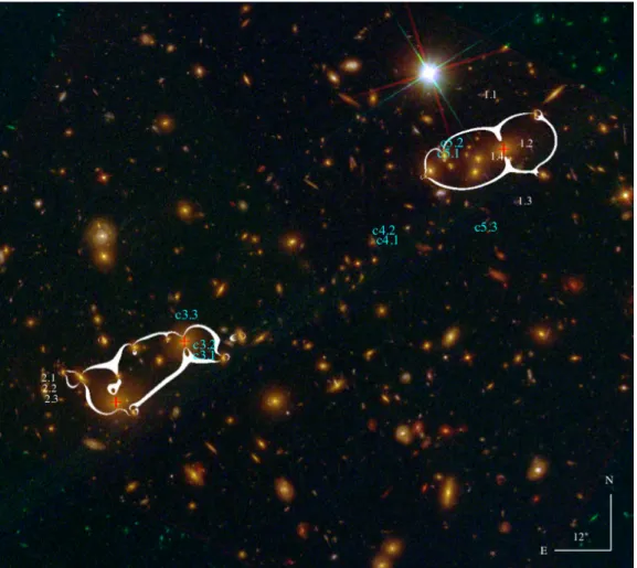
Fig. 1.—RELICS color image of MACS J0025.4-1222 (Blue=F435W, Green=F555W+F814W, Red=F105W+F125W+F140W+F160W). The white contours show the critical curves from our best-fit model, for a source atzspec= 2.38 (system 1). Multiple images considered in the modeling are labeled in white, while candidate systems (not used in the fit) are shown in cyan (see also Table3). The positions of the three main BCGs are marked with a red cross. We sometimes refer to the colors of multiple images with respect to these composite images.
comprising the 34 brightest MACS clusters (Ebeling
et al. 2010). MACS0159 is also one of only two RELICS
clusters that are part of theWong et al.(2013) rank of prominent lenses, based on SDSS luminous red galaxy data. The presence of an extended X-ray source detected as a filamentary structure was reported by Kotov &
Vikhlinin (2006), who analyzed the mass-temperature
relation of clusters atz ∼0.5. An extended and diffuse emission around the BCG was also observed in the radio
byGiacintucci et al.(2014), in an analysis searching for
radio minihalos in a sample of X-ray luminous clusters. For this cluster we made use of the available archival HST data from GO programs 11103 and 12166 (PI: Ebeling).
Abell S295, the third cluster we analyze, (AS295,Abell
et al. 1989), is located at z = 0.30. This cluster is also
known as SPT-CL J0245-5302 and ACT-CL J0245-5302, and is part of the sample comprising the 26 most massive clusters detected by their SZ effect in the SPT Survey
(Williamson et al. 2011). Edge et al. (1994) reported
the discovery of a giant arc, dubbed “the Mexican hat”, in the North-West region of the cluster, detected during optical follow-up of the ROSAT All-Sky Survey as part of an ESO Key Program. At that time the data revealed the presence of three knots in the arc. AS295 was also studied byMenanteau et al. (2010), who discussed
opti-cal and X-ray properties of the first ACT cluster sample and noted that this cluster is likely a merger. Further works which have included AS295 are the ones by Ruel
et al.(2014) andBayliss et al.(2016), who presented and
analyzed spectroscopic data for a sample of clusters de-tected in the SPT survey. For this cluster we used the available archival HST data from GO program 13514 (PI: Pacaud).
The last cluster we analyze here is Abell 697 (A697 hereafter,Abell et al. 1989;Crawford et al. 1995), a rich and massive cluster located at z = 0.282. This cluster is part of the ROSAT Brightest Cluster Sample (BCS,
Ebeling et al. 1998), being a hot and luminous cluster
in the X-ray. Kempner & Sarazin (2001) suggested the presence of a diffuse cluster-scale radio emission, later classified as a giant radio halo (Venturi et al. 2008). Sub-sequent radio, optical and X-ray analyses hint that A697 is the result of a complex multiple merger history occur-ring along the line-of-sight (Girardi et al. 2006;Macario
et al. 2010). This finding is supported by the first lens
SL models for four RELICS clusters 5
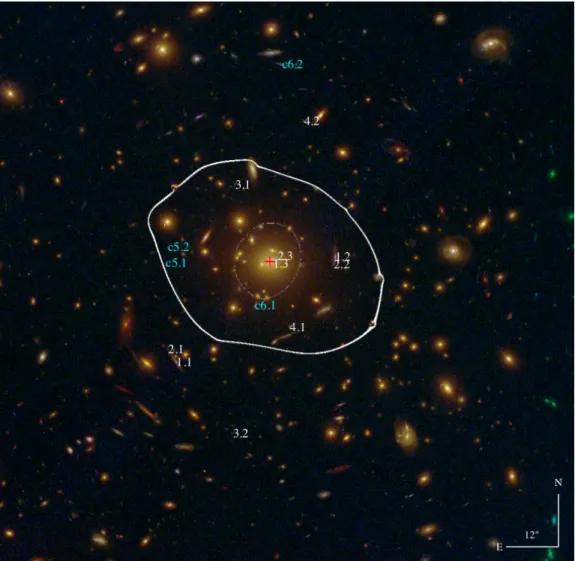
Fig. 2.—RELICS color image of MACS J0159.8-0849 (Blue=F435W, Green=F606W+F814W, Red=F105W+F125W+F140W+F160W). The white contours show the critical curves from our best-fit model, for a source atz= 1.55. Multiple images considered in the modeling are labeled in white, while candidate systems (not used in the fit) are shown in cyan (see also Table4). The BCG position is marked with a red cross.
3. LENS MODELING FORMALISM
We adopt a Light-Traces-Mass approach to model the projected central mass distribution of the clusters. One of the advantages of this approach is its prediction power, guiding the identification of multiple-image systems. The method relies on the simple assumption that the distri-bution of the observed galaxies traces the overall DM distribution of the cluster. In the following we give an overview of the method. For a detailed description we re-fer toZitrin et al.(2009,2015, see alsoBroadhurst et al.
2005).
The modeling starts with the construction of a cata-log of cluster members using the red sequence method
(Gladders & Yee 2000). For each cluster, we use the
magnitudes measured from the F606W and F814W fil-ters to draw the color-magnitude diagram, and identify the location of the red sequence. We typically consider galaxies to be cluster members when lying within ±0.3 mag of the sequence, selecting galaxies down to 23 AB. We follow this first selection with a visual inspection of the HST color image and manually exclude objects with a doubtful morphology or color. Similarly, we sometimes manually include galaxies that may have been lost in the initial selection. Additionally, the flux of a few galaxies,
typically, has to be reduced manually; especially galaxies that are designated as cluster members but show bright spiral structure, and so have in practice a significantly lower M/L than the one effectively adopted for cluster ellipticals. We discuss this point in some more detail in §5.
The next step is to construct the mass distribution based on the final catalog of selected cluster galaxies. We start by assigning a power-law surface mass-density radial profile to each galaxy:
Σ(r) =Kr−q. (1)
The amplitude of this profile,K, is linearly scaled with the observed luminosity. The power-law exponent q, is the same for all galaxies, and is a free parameter of the model. The enclosed mass of a galaxy within an angular distance θis then given by:
M(< θ) = 2πK 2−q(Dlθ)
2−q, (2)
and its deflection field is:
α(θ) = 4GM(< θ)
c2θ
Dls DlDs
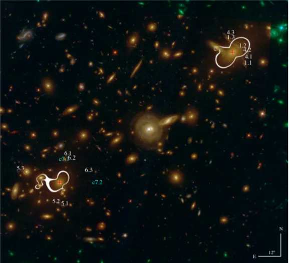
Fig. 3.—RELICS color image of Abell S295 (Blue=F435W, Green=F606W+F814W, Red=F105W+F125W+F140W+F160W). The critical curves for our best-fit model are shown in white, corresponding to a source at z = 1. Multiple images used in the modeling are labeled in white, while candidate systems (not used in the fit) are shown in cyan (see also Table5). For clarity we have omitted subset-systems 2 and 3 which are located in the giant arc very close to systems 1 and 4. The positions of the two BCGs are marked with red crosses.
whereDls,DlandDsare the angular diameter distances
between lens-source, observer-lens and observer-source respectively. The last equation can be rephrased and written as:
α(θ) =KqF θ1−q, (4)
where F is the measured flux, and Kq is a constant
that depends on the power-law indexqand encompasses all the previous constants and proportion relations. The deflection angle at a certain position due to all cluster member galaxies, α~gal, is given by a linear sum of all
individual galaxy contributions. The sum of all galaxy mass-density distributions therefore defines the galaxy component of the model, which should now be supple-mented by a DM distribution.
As the DM distribution should be smoother than the contribution of the galaxies, we apply a 2D Gaussian smoothing to the co-added galaxy component. We define
Sto be the width of the 2D Gaussian and the second free parameter of the model. The deflection field resulting from the smooth component is defined as ~αDM. The
overall normalization (essentially Kq) and the relative
weight of the galaxies to the DM component (which we denoteKgal), are two other free parameters of the model.
Since some difference is expected between the
distribu-tion of galaxies and DM, a two-parameter external shear is added to the deflection field for further flexibility (also, the external shear effectively introduces ellipticity to the magnification map). The external shear is described by its amplitude and its position angle, which are also free parameters of the model. The deflection field from the external shear is marked as α~ex. The basic model has
thus a total of six global free parameters.
The total deflection field is then obtained by adding the three components up and accounting for their relative contributions:
~
αT(~θ) =Kgal~αgal(~θ) + (1−Kgal)~αDM(~θ) +~αex(~θ). (5)
The model can be further improved, typically, by al-lowing the weight of few central, brightest cluster galax-ies (BCGs) to vary as free parameters. Similarly, a core radius and ellipticity can be intorduced to these BCGs, in order to improve the fit. In addition, redshifts of sys-tems lacking spectroscopic measurements can be left as free parameters and optimized in the fitting routine.
SL models for four RELICS clusters 7
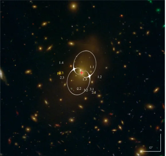
Fig. 4.—RELICS color image of Abell 697 (Blue=F435W, Green=F606W+F814W, Red=F105W+F125W+F140W+F160W). The white
contours show the critical curves for our best-fit model, for a source atz= 2. Multiple images displayed in white are labeled according to Table6. The position of a third counter image for system 3 predicted by the best-fit model is indicated in yellow. The BCG is marked with a red cross.
χ2=
n
X
i=1
(xmi −xobsi )2+ (yim−yiobs)2
σ2
i
, (6)
where xobsi , yobsi are the observed multiple-image posi-tions, xm
i , yim the corresponding coordinates predicted
by the model and σi the positional uncertainty. This
minimization quantifies the distance of the multiple im-age positions inferred by the model with respect to the observed ones (we assume here a positional uncertainty of 0.5”, e.g. Newman et al. 2013). To assess the uncer-tainty of the best-fit model we consider the rms of the reproduced images in the image plane:
rms=
v u u t
1
N n
X
i=1
(xm
i −x
obs
i )2+ (y
m
i −y
obs
i )2, (7)
given the predicted (xm
i , yim) and observed (xobsi , yiobs)
positions and the total numberN of multiple images. With only six global parameters, and relying on a sim-ple assumption, the Light-Traces-Mass method is a pow-erful tool to identify multiple images and probe the clus-ter mass distribution.
We start by constructing a preliminary model (using typical parameter values) based on the red-sequence clus-ter member selection and photometry. Thanks to the LTM assumption, this initial guess is sufficiently success-ful to guide the identification of multiple images, which are ultimately identified by eye, based on the morphol-ogy, position, and color information obtained from the HST images and compared with the model’s prediction. We search for new multiple-image candidates predicted by the model in an iterative way, refining the model in each step. For the final model, we only use the most secure systems, i.e. those that agreed with the model’s prediction and are conspicuously similar to the prediction and to each other in terms of symmetry, color, internal details, photometric redshift, etc.
a very good photo-z estimate, and leave the redshift of the other systems to be optimized in the minimization around the best-fit value of their photo-z probability dis-tribution function. This will be detailed for each cluster individually in§4.
4. INDIVIDUAL LENS MODELS
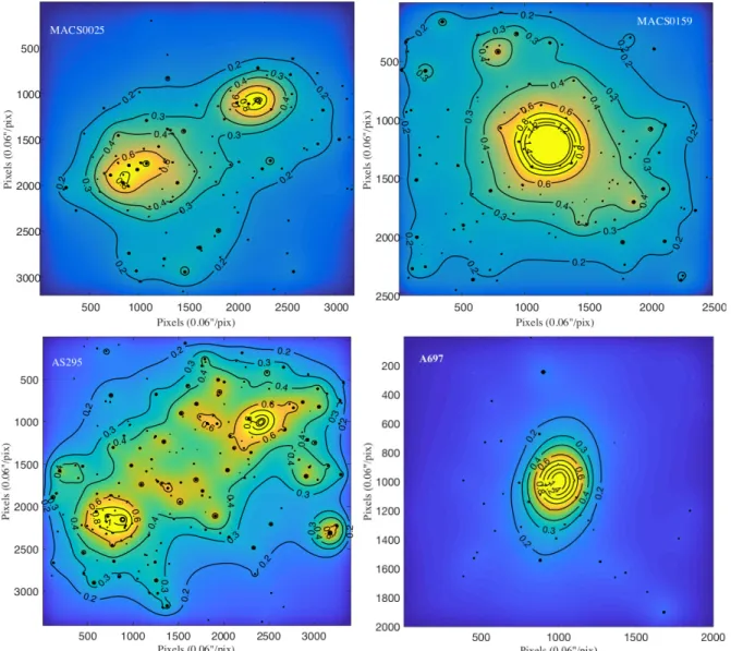
In the following subsections we present for each cluster the strong lens modeling and some of its immediate re-sults. The projected mass-density distributions from the best-fit models, for a source located atzs= 2, are shown
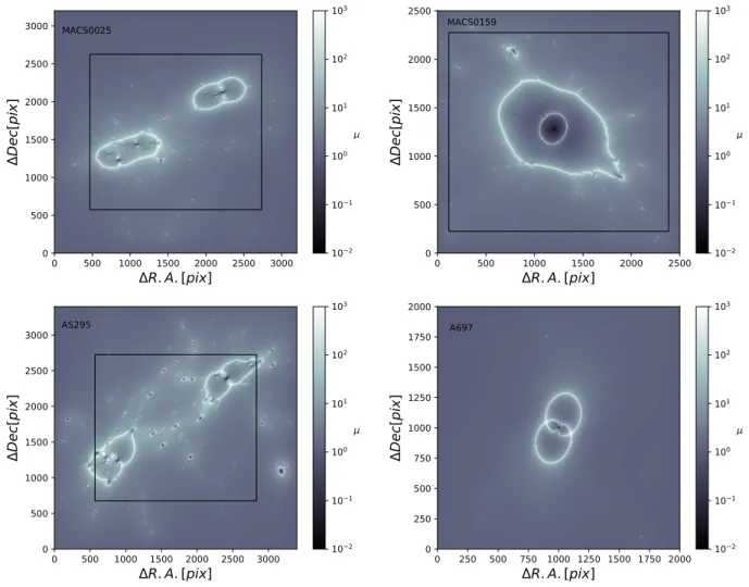
in Fig. 5, and the corresponding mass-density profiles are presented in Fig. 8. High-redshift magnification maps, scaled to a source redshift ofzs= 9, are shown in Fig. 6.
A list of the multiple image systems used as constraints can be found in AppendixA. We also list therein candi-date multiple images (labeled with a c). These are im-ages or systems whose identification was more ambiguous and were not included as SL constraints (for example, im-ages with similar color and/or morphology, but notable discrepancy between the observed and model-predicted location or orientation).
4.1. MACS J0025.4-1222
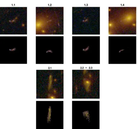
Our model for MACS0025 is constructed based on two systems of multiple images. System 1 forms at the North-Western subcluster and is composed of four counter im-ages showing a two-component morphology, which in-cludes a blue bright spot and a diffuse feature. Three images of this system were identified in Bradaˇc et al.
(2008) as system AB. Bradaˇc et al. (2008) also mea-sured a spectroscopic redshift for this system ofz= 2.38 using Keck/LRIS data. A second lens model by Zitrin
et al.(2011) has predicted a fourth image for this system,
which they also identified in the data and is used here. The second system we consider here was labeled system
C in Bradaˇc et al. (2008), and we define three multiple
images located on the east side of the main BCGs as con-straints. This system was also spectroscopically targeted
byBradaˇc et al.(2008), but did not yield a spectroscopic
redshift. Bradaˇc et al. (2008) estimated a photometric redshift ofzphot= 1.0+0−0..52for this system, due to the 4000
˚
A break possibly lying between the F555W and F814W bands. The BPZ estimate from RELICS gives a higher
zphot = 3.8 (corresponding to the value for the counter
images denoted as 2.2 and 2.3 here), a redshift which we fix for this system in our modeling. We note that this es-timate uses information from the seven HST band obser-vations available for RELICS, whileBradaˇc et al.(2008) used the information from the F450W/F555W/F814W bands available at the time. This choice of fixing both redshifts in our model was made in order to constrain both mass clumps.
Bradaˇc et al. (2008) also included a third system in
their SL model, labeled system D. Here we do not in-clude this as constraints. Based on the new information from our multi-band observations, the northern counter image in the region of the second BCG (labeled c3.3) does not seem to match the southern arc-shaped images (c3.1-2) in terms of color. In addition, our model does not precisely predict the northern counter image, nor the unexpected orientation of the southern arc. So we des-ignate this system as a candidate system only (labeled
as system c3). We note also that Zitrin et al.(2011) in-cluded a fourth two-image system that their older model agreed with. We decided to discard this system from our analysis as it appears to be a single elongated image with no counter image predicted by our model, and only mention for completeness as a candidate system (c4).
In our modeling we include the weight of the north-western BCG as a free parameter to be optimized, al-lowing it to vary with respect to the original M/L ratio. We set the ellipticity and position angle for this BCG to the values given by SExtractor. The resulting criti-cal curves, computed for a source at z = 2.38, and the location of the multiple images, can be seen in Fig. 1.
The multiple image reproduction is shown in Fig. 9. Our model precisely predicts the four counter images of system 1 with respect to the position and orientation. The prediction for system 2 returns an arc-shaped image with the orientation matching the observed disposition of the system counter images, although the specific po-sition of the predicted images is less accurate, and likely influenced by the local cluster member around which the arc partially revolves. We acknowledge that given the lack of internal details in system 2, its exact configura-tion remains ambiguous. The final rms of the best-fit model is 0.57”.
Due to the small number of constraints, i.e., multiple images that could be reliably identified, the model for MACS0025 is in a sense, a simple model, with a minimum number of free parameters. Future use of the presented lens model should thus acknowledge its limitations.
4.2. MACS J0159.8-0849
We identify four multiple-image systems in MACS0159, with which we construct our model. The first and the second systems represent different constraints related to the same source (although it is unclear if the source is one or, e.g., two merging galaxies). The third system shows a distinctive green color – in the color-composite RELICS HST image – that aided in its identification, and the fourth system corresponds to a small, relatively bright source.
We set the main source to be atz= 1.55, correspond-ing to the mean zphotfrom the counter images 1.1 and 1.2
(the more reliable BPZ estimates, since image 1.3 suffers contamination from the BCG light), and fix the redshift of systems 1 and 2 to this value. The redshifts of systems 3 and 4 are left as free parameters to be constrained by the model.
The mass distribution of the cluster is modeled with both the weight and the core radius of the BCG as free parameters, where the latter can reach values up to 100 kpc. Our best-fit model does not include an ellipticity for the BCG, which seems to be fairly spherical.
SL models for four RELICS clusters 9
Fig. 5.— Convergence map of each cluster produced from our best-fit models. The maps show the projected surface mass-density distribution in units of the critical density for lensing, for a source atz= 2. The orientations are the same as in Figures 1-4.
4.3. Abell S295
The modeling of AS295 is based on the identification of six sets of constraints. The first four are part of a known giant arc located in the north-west region of the cluster, close to the BCG. These four subsets can be dis-tinguished by the differences in their color and relative positions, where we identify three multiple images for each set. The arc has a spectroscopic redshift of 0.93 re-ported in the literature (Edge et al. 1994), and we adopt this value for all four subsets related to the arc.
The two other systems (Systems 5 and 6) are found in the south-east concentration of galaxies. These are new identifications, with three multiple images each. System 5 has an elongated image on the east and two counter images lying close to each other, south of the BCG. Be-tween these two images there is an additional faint galaxy that might locally contribute somewhat to the lensing as well. System 6 is a faint and long arc, north-west of the respective BCG. For these systems there is no spectro-scopic redshift measurements available, so we leave their redshifts as free parameters of the model. We note that while we refer to systems 5 and 6 as secure here since they match the model’s prediction, they lack clear
inter-nal details and thus their identification should be taken with slightly more caution.
Our model for AS295 has the weight of the two BCGs as free parameters to be optimized in the minimiza-tion. For the Northern BCG we set the ellipticity and position angle to the values given by
SExtrac-tor. The Southern BCG presents a spherical
mor-phology and so we decided not to apply an ellipticity. The weight of two bright, spiral-looking cluster mem-bers (RA = 02:45:25.710, Dec = -53:01:43.031 and RA = 02:45:37.573, Dec=-53:02:58.595) lying near the two BCGs, was reduced by factor of 2 (this slightly improved the reproduction of multiple images; see also discussion in §5.1 for MACS0025).
0 500 1000 1500 2000 2500 3000
R. A. [pix]
0 500 1000 1500 2000 2500 3000
De
c[p
ix]
MACS0025 102 101 100 101 102 1030 500 1000 1500 2000 2500
R. A. [pix]
0 500 1000 1500 2000 2500De
c[p
ix]
MACS0159 102 101 100 101 102 1030 500 1000 1500 2000 2500 3000
R. A. [pix]
0 500 1000 1500 2000 2500 3000
De
c[p
ix]
AS295 102 101 100 101 102 1030 250 500 750 1000 1250 1500 1750 2000
R. A. [pix]
0 250 500 750 1000 1250 1500 1750 2000
De
c[p
ix]
A697 102 101 100 101 102 103Fig. 6.—Magnification maps for the four RELICS clusters analyzed in this work. The maps show the expected magnification distribution for a source located atz= 9, from our best-fit models. The orientations are the same as in Figures 1-4. The pixel scale is 0.06”/pixel. Black squares represent the WFC3/IR field-of-view (136”×123”). For A697 our FoV is fully encompassed within the WFC3/IR FoV.
11.
The resulting critical curves from our best-fit model (for a source redshift of z= 1), along with the multiple images, are seen in Fig. 3.
4.4. Abell 697
We construct the model for A697 using three multiple-image systems. Because there is no spectroscopic redshift available for any of the systems, we fix the main source redshift to the value of the system with the most reliable photometric-redshift estimate (corresponding to system 1), leaving the redshift of the remaining systems as free parameters.
The first system corresponds to a blue source showing a distinct morphology, leading to a reliable identifica-tion of four counter images well predicted by our model. The second system is also a blue-looking galaxy and we identify three counter images south and south-east of the BCG. The third is an arc-shaped object lying south of the cluster center, for which we identify two multiple images. This system was previously reported in the literature by
Metzger & Ma (2000), who has estimated a lower limit
for the redshift of the source ofz >1.3 by combining the arc spectrum and its color.
Our model for A697 allows the weight of the BCG to vary as a free parameter, as well as its ellipticity and
position angle. The source redshift for system 1 is set to the mean of thezphotdistributions of images 1.2 and 1.4
(as image 1.1 suffers contamination from the BCG light and for image 1.3 there was no zphot solution found).
Redshifts for systems 2 and 3 are allowed to vary and are optimized by the minimization procedure. Our best-fit model yields a redshift of z= 2.97+0−0..0438for system 3, consistent with the lower limit found byMetzger & Ma
(2000) within 1σ.
The final model reproduces well systems 1 and 2. For system 1 it also predicts a smaller fifth counter image very close to the BCG that we can not identify, possible due to the contamination by the BCG light. The model correctly predicts the arc-shape and orientation of system 3, and as expected from the lensing symmetry it also predicts a third, fainter counter image on the east side of the cluster center that we do not securely identify. The reproduction of multiple images by the best-fit model, which has a final rms of '0.8200, is shown in Fig. 12. The resulting critical curves for a source atz= 2 and the multiple images used as constraints are shown in Fig. 4.
5. RESULTS AND DISCUSSION
5.1. Lens modeling results
SL models for four RELICS clusters 11
distribution (Figs. 1, 5), in agreement with the find-ings by Bradaˇc et al. (2008) and Zitrin et al. (2011). Such morphology supports the picture that this cluster is undergoing a major merger (Bradaˇc et al. 2008; Ma
et al. 2010). The Einstein radius obtained from the
modeling for the North-Western subcluster is θE(z =
2) = 8.1±0.8” and encloses a mass of M = 1.60± 0.24×10¹³M, while for the South-Eastern
substruc-ture we foundθE(z= 2) = 7.2±0.7” and enclosed mass M = 1.18±0.18×10¹³M
. Note thatZitrin et al.(2011)
reported a substantially larger radius for MACS0025, of
θE= 30±2” forz= 2.38. Our model is similar to theirs
around the North-Western subclump, but implies a much smaller critical curve around the main (South-Eastern) clump (as can be seen by comparing Fig. 3 fromZitrin
et al.(2011) to our Fig. 1). Our model was constructed
with two major differences compared with the previous model byZitrin et al.(2011). First, as was implied by the RELICS data, here we assign a significantly higher red-shift for System 2, so that the critical curves of the main mass clump are required to be smaller per given redshift. The second difference is the lower weight manually given by us to some of the bright galaxies around the South-Eastern main clump. Specifically, these are (apparently) cluster galaxies, that show bright spiral structure, and therefore seem to significantly deviate from the general, early-type cluster member M/L ratio, in the sense that they are about an order of magnitude too bright for their actual mass contribution compared to cluster ellipticals
(Maraston 2005;Courteau et al. 2014;Bahcall & Kulier
2014). We therefore manually reduced the mass (i.e. in-put flux) of these galaxies by a factor of 10. 20
MACS0159 is a massive X-ray selected lens and has the largest (single-clump) Einstein radius among the clusters analyzed in this work, corresponding to θE(z = 2) =
24.9±2.5”. The mass inside the critical curves corre-sponds toM = 1.15±0.17×10¹⁴M
. Our model exhibits
a fairly round and regular morphology (Fig. 5), which together with the regular X-ray morphology (Maughan
et al. 2008) might indicate that this is a relaxed cluster.
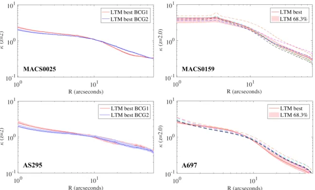
The central flattening in the projected mass density pro-file seen in Fig. 8 (top-right), may be, in part, a result of the superposition of other elliptical cluster members onto the BCG (Fig. 2).
The model for AS295 shows a bimodal mass distribu-tion, following the cluster galaxy concentrations (Figs.
3, 5). The North-Western clump hosting the giant arc has an Einstein radius of θE(z = 2) = 12.6±1.3”, and
mass ofM = 1.96±0.29×10¹³Menclosed by the
criti-cal curves. For the South-Eastern subcluster our best-fit model gives an Einstein radius ofθE(z= 2) = 12.7±1.3”
and an enclosed mass ofM = 2.04±0.31×10¹³M .
Our analysis for A697 implies a rather elliptical mass distribution in projection (Fig. 5), and elongated critical curves (Fig. 6). The Einstein radius given by the model isθE(z= 2) = 11.1±0.1” and the critical curves
encom-pass a total mass of M = 1.45±0.23×10¹³M . The
somewhat-elliptical nature of the lens found in our
anal-20 Note, this estimate is subjective and based on our
experi-ence in a previous analysis of a large sample of clusters, e.g.,Zitrin
et al. (2015). Nonetheless, once their weight has been
substan-tially reduced, their exact mass contribution is not of particular importance.
10
010
110
210
210
110
010
1Cu
m
ula
tiv
e a
re
a (
>
) [
ar
cm
in
2]
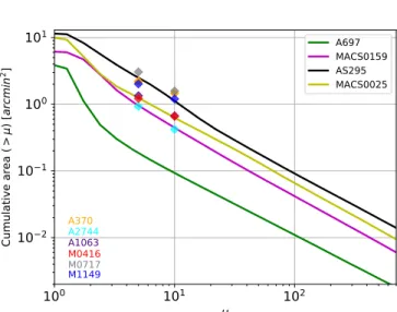
A370 A2744 A1063 M0416 M0717 M1149 A697 MACS0159 AS295 MACS0025Fig. 7.—The image-plane area above each magnification value as a function of magnification value, for each of the analyzed clus-ters. The magnification is computed for a source redshift ofz= 9. Diamonds indicate the cumulative area withµ≥5 andµ≥10 for the HFF clusters (considering the LTM-Gauss models).
ysis agrees with the model from Metzger & Ma (2000), with the BCG orientation, and with the X-ray morphol-ogy reported in Girardi et al. (2006), which reinforces the possible recent-merger scenario.
5.2. Implications for high-redshift studies
5.2.1. Lensing strength
Galaxy clusters with large Einstein radii and those that entail a large area of high magnification are objects of particular interest in the search for high-z galaxies (e.g.,
Zheng et al. 2012; Zitrin et al. 2014; Kawamata et al.
2016). One way to evaluate the lensing strength of a lens is through the total area, A, in the source plane or the image plane, that has a magnification above a certain value, as a function of the magnification value (a plot of
A(> µ) versus µ). This area is sometimes referred to as the cumulative area above a certain magnification (e.g.,
Cerny et al. 2017), a term we use here as well. In Fig. 7
we show such cumulative magnification curves computed from our best-fit models, for a source located at redshift
zs = 9. We also present therein the cumulative areas
of the HFF clusters, specifically, for µ≥ 5 and µ ≥10 (adopting the Zitrin-LTM-Gauss models, as these were constructed with similar formalism as the one used here). Among the four clusters, AS295 shows the largest high magnification area, almost comparable to the largest HFF clusters, as can be seen in Fig. 7(see alsoJohnson
et al. 2014). However, given the lack of spectroscopic
Ein-MACS0025 MACS0159
AS295 A697
Fig. 8.—Radial mass-density profiles scaled toz= 2 for the RELICS clusters analyzed in this work. For MAC0025 and AS295 we show the profile around the BCG of each subcluster, namely BCG1 for the Northern-Western clump and BCG2 for the South-Eastern clump. For the clusters lacking of zspec, MACS0159 and A697, we also present profiles computed by assuming different redshifts for the main system together with the result of the best-fit model, shown by the solid red line together with the 68.3% confidence level represented by the shaded red region. Cyan and green lines corresponds to a change of−10%,+10% in redshift, respectively, magenta and blue lines to
−25%,+25% and orange and black to a variation of−50%,+50% respectively. stein radius, and in addition a smaller area of high
mag-nifications, is not surprising. As can be seen for example in Fig. 6, merging clusters create an area of high mag-nification between the merging subclumps (in addition to, or because of the lensing strength of each subclump individually). This means that although the total criti-cal area (summed over the subclumps) can be modest or even small, merging clusters, projected on the plane of the sky, will often show large areas of high magnification. The fact that the two largest cumulative areas of high magnification found in our analysis correspond to the two clusters showing substructures demonstrates this idea. Note that the HFF clusters are also, similarly, merging clusters. The impact of cluster mergers on lensing prop-erties has been examined before. It has been found that merging clumps boost the critical area - and the number of multiple images in case the subclumps are close enough - forming the most useful strong gravitational lenses (see e.g., Torri et al. 2004; Meneghetti et al. 2007; Redlich
et al. 2012;Zitrin et al. 2013), especially if also the
criti-cal curves are relatively large as is the case for the HFF clusters. In that sense, the lensing strength estimate by the cumulative area alone might be misleading. Merg-ing clusters, such as those of the HFF which have both large enough critical areas and also large high magnifica-tion areas, are preferable at least for two reasons: first, they will be rich in multiple images and are thus much better modeled. Second, if the subclumps are too small or distant so that the critical curves do not merge and the critical area remains effectively small – such as for MACS0025 and AS295 here – the area of high magnifi-cation, even if large, will also be highly sheared, so that background galaxies will be significantly stretched
per-pendicular to the axis connecting the two subclumps. It has been found that high shear can significantly hinder the detection of magnified high-redshift galaxies (Oesch
et al. 2015;Bouwens et al. 2017a). If the critical area is
large enough, multiple images of the background sources will typically appear, and so the combination of a large high magnification area and large enough critical area seems crucial for maximizing the detection of intrinsi-cally faint high-redshift objects. In that sense, we con-clude that the intrinsically “best lens” in our four cluster sample, is likely MACS0159.
We also note that the cumulative-area comparison (Fig. 7) to estimate the lensing strength is sometimes more insightful if the same field-of-view (FOV) is probed in all clusters (for example it is often comfortable to de-fine the WFC3/IR FOV, in the case of HST imaging), es-pecially if the goal is to plan observations and estimate the expected number of objects per FOV. Here, how-ever, our goal is to maximize the area probed for each cluster and so we simply consider the full FOV used for the modeling, which differ somewhat from one another (the A(µ= 0) points in Fig. 7 represent the total area modeled for each cluster). The somewhat different FOV sizes, however, mostly affect the areas with low magni-fications, as high magnifications are generally induced only near the center and are thus included in any case (increasing the FOV will shift the A(µ = 0) point but will hardly affect the A(> µ= 10) point, for example).
Another related important point is why A697 is a rel-atively small lens, given it is the tenth most massive SZ-mass cluster in the Planck catalog (Planck Collaboration
et al. 2016a). While massive, often merging, bright X-ray
excep-SL models for four RELICS clusters 13
tional strong lenses (e.g.,Zitrin et al. 2013, and references therein), it should be examined more statistically if the scatter on SZ-mass, usually estimated through X-ray or weak-lensing mass scaling relations, is an equal indicator for SL strength. It is also possible that the SZ signal in this case was boosted by an underlying radio source
(Kempner & Sarazin 2001;Venturi et al. 2008; Macario
et al. 2010). We leave these issues to be examined in
other, future work.
5.2.2. RELICS high-redshift candidates
The first sample of high-z galaxy candidates detected in RELICS clusters was recently presented by Salmon
et al. (2017). In relation to the clusters analyzed in
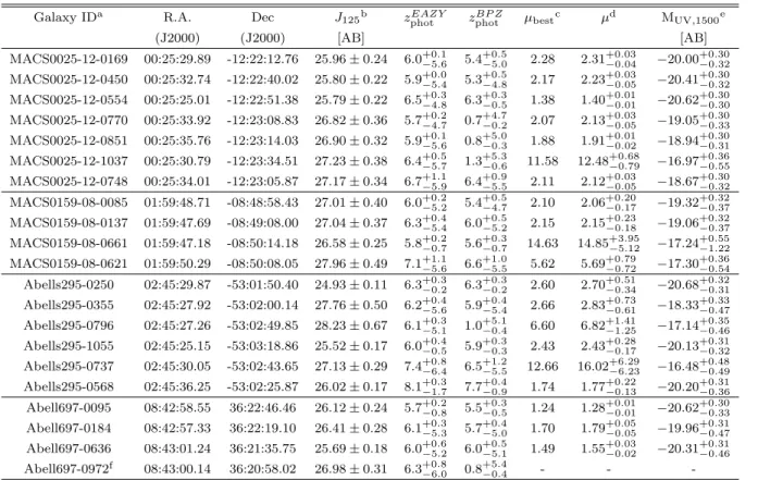
this work, Salmon et al. (2017) found six candidates in MACS0025, three in MACS0159, four in AS295 and four in A697, in the redshift range 6 ≤zphot ≤8. The
pho-tometric redshifts are estimated with both the BPZ, and Easy and Accurate Z (EAZY,Brammer et al. 2008). The candidates are presented in Table2, following the nota-tion fromSalmon et al.(2017). Here, we provide magni-fication estimates for the candidates. In table2we quote the best-fit magnification from our models, (correspond-ing to the minimumχ2), the average magnification from
the MCMC, and the 68.3% confidence interval obtained from a 100 random realizations from the MCMC fitting. Absolute magnitudes Muv at the rest-frame λr = 1500
˚
A are computed for the candidates based on a fit to the UV continuum slope using the WFC3/IR bands (F105W, F125W, F140W, F160W), assuming the flux follows a power-law relation fλ ∝ λβ (e.g., Meurer et al. 1999).
The final absolute magnitude is then obtained from the flux at (1 +z)λr.
Based on our models we also checked for – but did not find – any potential multiple image systems consis-tent with the reported high-redshift candidates among the analyzed clusters.
5.3. Redshift and other uncertainties
A critical point in the construction of a SL model is the knowledge of the relative cosmological distances be-tween observer, lens and source. The lack of spectro-scopic information for the lensed galaxies may bias the final mass distribution and magnification maps derived from SL constraints (Smith et al. 2009; Johnson et al.
2014; Johnson & Sharon 2016). Two of our clusters,
MACS0159 and A697, do not have any spectroscopic in-formation available for multiple-image systems, and we fixed the redshift of the source with the most reliable photo-z estimate (we often call this the ”main source”, the source the model is primarily calibrated to). The other two clusters, MACS0025 and AS295, have one sys-tem each with spectroscopic redshift available from the literature (Bradaˇc et al. 2008;Edge et al. 1994), to which our models are calibrated.
Aside from MACS0025, for which we built a simple model based on two multiple-images systems with both redshifts fixed, for the other clusters we only fix the main source redshift and leave the redshift of the other sys-tems to be constrained in the minimization, adopting a broad prior range (typically±0.3 in the relativeDls/Ds
ratio). Given the uncertainties in source redshifts, it is essential to examine how such uncertainties affect our
final solutions, especially for the two clusters that lack any spectroscopic redshifts (MACS0159 and A697). For these two clusters we conducted a series of tests where we shifted the main source redshift by±10%,±25% and ±50% from its original photo-z value. The resulting mass density profile for each model is shown in Fig. 8 (right panels), together with the best-fit and 1σinterval of our best-fit models. Despite the expected variation in the ra-dial mass profiles, the results show overall an agreement with our best-fit models within 3σin most of the radial range. Differences exceeding the 3σ level for A697 oc-cur at the very central region and at intermediate radius (around ∼ 8”), where the errors on the best-fit profile are particularly small. For MACS0159 the extreme case
of a −50% shift results in a higher profile above the 3σ
level in all scales.
We use the same suite of trial models to examine the effect of lack of spectroscopic redshifts also on the power of the lens (i.e., the cumulative magnification area). We find that the redshift uncertainties typically propagate into a difference of up to±50% percent in the cumulative area of the lens with high magnification (for example, aboveµ >5 orµ >10). The exception, as expected from the density profiles results, is the case of a−50% change in redshift. In this case the area of high magnification can be increased by up to 100% for both MACS0159 and A697. We note, however, that this most extreme effect increases the lensing strength, indicating that our magnification estimate is conservative. The impact of redshift errors is generally smaller in areas with lower magnification values. In a similar fashion, for example,
Cerny et al.(2017) found for several clusters that about
90% of their modeled FOV (20000×20000) was typically constrained to better than ∼20−40%.
Other sources of systematic uncertainties in SL models include the non-correlated matter along the line-of-sight
(Seljak 1994; Puchwein & Hilbert 2009;D’Aloisio et al.
2014; Bayliss et al. 2014), the choice of parametrization
(Zitrin et al. 2015;Meneghetti et al. 2017), identification
of false multiple-image systems (Bradaˇc et al. 2008), the mass-sheet degeneracy (Falco et al. 1985; Bradaˇc et al.
2004; Liesenborgs & De Rijcke 2012) and uncertainties
in the adopted cosmology (Bayliss et al. 2015). The un-derstanding of systematics is central for studies based on strong lens models such as measurements of the high-z luminosity function, which relies on the determination of intrinsic properties of lensed galaxies and of the effective volume. Such uncertainties should be taken into account when propagating results based on SL models, and we refer the reader to the above works for further discussion on these.
TABLE 2 High-z (z∼6) candidates
Galaxy IDa R.A. Dec J125b zEAZY
phot zphotBP Z µbestc µd MUV,1500e
(J2000) (J2000) [AB] [AB]
MACS0025-12-0169 00:25:29.89 -12:22:12.76 25.96±0.24 6.0+0−5..16 5.4−+05..05 2.28 2.31−+00..0304 −20.00+0−0..3032 MACS0025-12-0450 00:25:32.74 -12:22:40.02 25.80±0.22 5.9+0−5..04 5.3
+0.5
−4.8 2.17 2.23 +0.03
−0.05 −20.41 +0.30 −0.32 MACS0025-12-0554 00:25:25.01 -12:22:51.38 25.79±0.22 6.5+0−4..38 6.3
+0.3
−0.5 1.38 1.40 +0.01
−0.01 −20.62 +0.30 −0.30 MACS0025-12-0770 00:25:33.92 -12:23:08.83 26.82±0.36 5.7+0−4..27 0.7−+40..27 2.07 2.13−+00..0305 −19.05+0−0..3033 MACS0025-12-0851 00:25:35.76 -12:23:14.03 26.90±0.32 5.9+0−5..16 0.8−+50..30 1.88 1.91−+00..0102 −18.94+0−0..3031 MACS0025-12-1037 00:25:30.79 -12:23:34.51 27.23±0.38 6.4+0−5..57 1.3
+5.3
−0.6 11.58 12.48 +0.68
−0.79 −16.97 +0.36 −0.55 MACS0025-12-0748 00:25:34.01 -12:23:05.87 27.17±0.34 6.7+1−5..19 6.4
+0.9
−5.5 2.11 2.12 +0.03
−0.05 −18.67 +0.30 −0.32 MACS0159-08-0085 01:59:48.71 -08:48:58.43 27.01±0.40 6.0+0−5..22 5.4
+0.5
−4.7 2.10 2.06 +0.20
−0.17 −19.32 +0.32 −0.37 MACS0159-08-0137 01:59:47.69 -08:49:08.00 27.04±0.37 6.3+0−5..44 6.0
+0.5
−5.2 2.15 2.15 +0.23
−0.18 −19.06 +0.32 −0.37 MACS0159-08-0661 01:59:47.18 -08:50:14.18 26.58±0.25 5.8+0−0..27 5.6−+00..73 14.63 14.85−+35..9512 −17.24+0−1..5522 MACS0159-08-0621 01:59:50.29 -08:50:08.05 27.96±0.49 7.1+1−5..16 6.6−+15..50 5.62 5.69−+00..7972 −17.30+0−0..3654 Abells295-0250 02:45:29.87 -53:01:50.40 24.93±0.11 6.3+0−0..32 6.3−+00..23 2.60 2.70−+00..5134 −20.68+0−0..3231 Abells295-0355 02:45:27.92 -53:02:00.14 27.76±0.50 6.2+0−5..46 5.9−+05..44 2.66 2.83−+00..7361 −18.33+0−0..3347 Abells295-0796 02:45:27.26 -53:02:49.85 28.23±0.67 6.1+0−5..31 1.0
+5.1
−0.4 6.60 6.82 +1.41
−1.25 −17.14 +0.35 −0.46 Abells295-1055 02:45:25.15 -53:03:18.86 25.52±0.17 6.0+0−0..45 5.9
+0.3
−0.3 2.43 2.43 +0.28
−0.17 −20.13 +0.31 −0.32 Abells295-0737 02:45:30.05 -53:02:43.65 27.13±0.29 7.4+0−6..84 6.5−+15..52 12.66 16.02−+66..2923 −16.48+0−0..4849 Abells295-0568 02:45:36.25 -53:02:25.87 26.02±0.17 8.1+0−1..37 7.7−+00..94 1.74 1.77−+00..2213 −20.20+0−0..3136
Abell697-0095 08:42:58.55 36:22:46.46 26.12±0.24 5.7+0−0..28 5.5 +0.3
−0.5 1.24 1.28 +0.01
−0.01 −20.62 +0.30 −0.33 Abell697-0184 08:42:57.33 36:22:19.10 26.41±0.28 6.1+0−5..33 5.7−+05..04 1.70 1.79−+00..0505 −19.96+0−0..3147 Abell697-0636 08:43:01.24 36:21:35.75 25.69±0.18 6.0+0−5..62 6.0
+0.5
−5.1 1.49 1.55 +0.03
−0.02 −20.31 +0.31 −0.46 Abell697-0972f 08:43:00.14 36:20:58.02 26.98±0.31 6.3+0.8
−6.0 0.8 +5.4
−0.4 - -
-aFollowingSalmon et al.(2017) notations. bApparent magnitude in the F125W band. cMagnification from the best-fit model.
dMean magnification and 1σerrors from 100 random MCMC realizations.
eAbsolute magnitude atλ= 1500 ˚A. Errors include the uncertainty in the fit to the UV slope and propagated photometric and
magnifi-cation errors.
fOutside the modeled FOV.
6. SUMMARY
Observing 41 massive clusters with HST and Spitzer, the treasury RELICS program was primarily designed to find magnified high-z candidates, some of which are ex-pected to be apparently bright enough for future spectro-scopic follow-up from the ground and with JWST (e.g.,
Salmon et al. 2017;Acebron et al. 2018). SL models for
the clusters are crucial for studying the magnified sources and, for example, for deriving their intrinsic brightness (Table2), or star-formation properties, or for construct-ing the high-redshift luminosity function.
In this work we have presented SL models for four RELICS clusters. Our analysis, based on the Light-Traces-Mass approach whose main advantage is its pre-dictive power for finding multiple images, supplies the first published SL models for AS295 and for MACS0159. For A697 and MACS0025 we present improved mod-els thanks to the new RELICS data. In our model-ing we used as constraints both some previously known (in MACS0025, A697, AS295), and, importantly, several new identifications (in MACS0159, A697, AS295) of mul-tiply imaged galaxies.
Out of the four clusters we analyzed, AS295 has the largest cumulative area of high magnification, possibly as large as that of the largest HFF clusters (Fig. 7). This is much thanks to its two merging subclumps, which create
a large region of high magnification between them (Fig.
6; much of the region is outside each subclump’s criti-cal curves). Our analysis also indicates that MACS0025 is a highly magnifying lens, with cumulative area of high magnification comparable to the typical HFF clus-ter (Fig. 7). Also in the case of MACS0025 there is only a small critical area around each subclump, and most of high magnification area forms between the two sub-clumps. In that sense it should be noted that a large area of high magnification alone may not be sufficient for significantly enhancing the detection of high-redshift galaxies, and a sizable critical area – as was the case for the HFF clusters – is also important. MACS0159 is the largest main-clump lens in the sample we analyze here, with an Einstein radius ofθE= 24.9±2.5” (for a source
atzs= 2), and also has a significant, HFF-like area with
high magnification. It is thus likely the most efficient lens amongst the four clusters we analyze here. A697, despite signatures of recent galaxy interaction with the BCG, or suggested merger scenarios along the line of sight (Macario et al. 2010; Girardi et al. 2006), seems fairly regular in terms of SL, and constitutes the small-est lens in our sample, as well as the one with smallsmall-est area of high magnification.
SL models for four RELICS clusters 15
with extra care until more spectroscopic redshifts become available.
To address the uncertainties in our SL models that arise from the lack of spectroscopic information for the lensed sources we performed a suite of tests. We con-structed different lens models with a range of input red-shifts that deviate from the photo-z fiducial value used in our modeling, and examined the effect on the resulting density profile and on the lens power (cumulative area of high magnification). For most of the cases, the den-sity profiles of the trial models are within the 3σ confi-dence level of our best-fit model. Deviations above the 3σ
level are seen for A697 at small radii and for MACS0159 when applying a redshift change of−50%. Regarding the magnification values, the difference between the models are typically up to 50% in the cumulative area for high magnifications (µ > 5 and µ > 10). A refinement of the models, especially with respect to these systematics stemming from unavailable redshift information, will be
possible with future spectroscopic follow-up.
The lens models we presented here, including mass-density, shear and magnification maps, are made avail-able through the MAST archive.
This work is based on observations taken by the RELICS Treasury Program (GO-14096) with the NASA/ESA HST. Program GO-14096 is supported by NASA through a grant from the Space Telescope Science Institute, which is operated by the Association of Uni-versities for Research in Astronomy, Inc., under NASA contract NAS5-26555. This work was performed in part under the auspices of the U.S. Department of Energy by Lawrence Livermore National Laboratory under Con-tract DE-AC52-07NA27344. RCL acknowledges support from an Australian Research Council Discovery Early Career Researcher Award (DE180101240).
REFERENCES
Abell, G. O., Corwin, Jr., H. G., & Olowin, R. P. 1989, ApJS, 70, 1
Acebron, A., Cibirka, N., Zitrin, A., et al. 2018, ArXiv e-prints, arXiv:1803.00560
Applegate, D. E., von der Linden, A., Kelly, P. L., et al. 2014, MNRAS, 439, 48
Atek, H., Richard, J., Kneib, J.-P., et al. 2015, ApJ, 800, 18 Bahcall, N. A., & Kulier, A. 2014, MNRAS, 439, 2505 Barkana, R., & Loeb, A. 2001, Phys. Rep., 349, 125
Bartelmann, M. 2010, Classical and Quantum Gravity, 27, 233001 Bayliss, M. B., Johnson, T., Gladders, M. D., Sharon, K., &
Oguri, M. 2014, ApJ, 783, 41
Bayliss, M. B., Sharon, K., & Johnson, T. 2015, ApJ, 802, L9 Bayliss, M. B., Ruel, J., Stubbs, C. W., et al. 2016, ApJS, 227, 3 Beckwith, S. V. W., Stiavelli, M., Koekemoer, A. M., et al. 2006,
AJ, 132, 1729
Ben´ıtez, N. 2000, ApJ, 536, 571
Ben´ıtez, N., Ford, H., Bouwens, R., et al. 2004, ApJS, 150, 1 Benitez, N., Dupke, R., Moles, M., et al. 2014, ArXiv e-prints,
arXiv:1403.5237
Bertin, E., & Arnouts, S. 1996, A&AS, 117, 393
Bleem, L., Brodwin, M., Ashby, M., et al. 2014, Spitzer Imaging of Massive zgt1 SZ-Selected Galaxy Clusters, Spitzer Proposal Bouwens, R. J., Illingworth, G. D., Oesch, P. A., et al. 2017a,
ApJ, 843, 41
Bouwens, R. J., Oesch, P. A., Illingworth, G. D., Ellis, R. S., & Stefanon, M. 2017b, ApJ, 843, 129
Bouwens, R. J., Illingworth, G. D., Oesch, P. A., et al. 2015, ApJ, 803, 34
Bradaˇc, M., Allen, S. W., Treu, T., et al. 2008, ApJ, 687, 959 Bradaˇc, M., Lombardi, M., & Schneider, P. 2004, A&A, 424, 13 Bradley, L. D., Trenti, M., Oesch, P. A., et al. 2012, ApJ, 760, 108 Bradley, L. D., Zitrin, A., Coe, D., et al. 2014, ApJ, 792, 76 Brammer, G. B., van Dokkum, P. G., & Coppi, P. 2008, ApJ,
686, 1503
Broadhurst, T., Takada, M., Umetsu, K., et al. 2005, ApJ, 619, L143
Bromm, V., & Yoshida, N. 2011, ARA&A, 49, 373
Cerny, C., Sharon, K., Andrade-Santos, F., et al. 2017, ArXiv e-prints, arXiv:1710.09329
Clowe, D., Bradaˇc, M., Gonzalez, A. H., et al. 2006, ApJ, 648, L109
Clowe, D., Gonzalez, A., & Markevitch, M. 2004, ApJ, 604, 596 Coe, D., Ben´ıtez, N., S´anchez, S. F., et al. 2006, AJ, 132, 926 Coe, D., Bradley, L., & Zitrin, A. 2015, ApJ, 800, 84 Coe, D., Zitrin, A., Carrasco, M., et al. 2013, ApJ, 762, 32 Courteau, S., Cappellari, M., de Jong, R. S., et al. 2014, Rev.
Mod. Phys., 86, 47
Crawford, C. S., Edge, A. C., Fabian, A. C., et al. 1995, MNRAS, 274, 75
D’Aloisio, A., Natarajan, P., & Shapiro, P. R. 2014, MNRAS, 445, 3581
Dijkstra, M. 2014, PASA, 31, e040
Ebeling, H., Barrett, E., Donovan, D., et al. 2007, ApJ, 661, L33 Ebeling, H., Edge, A. C., Bohringer, H., et al. 1998, MNRAS,
301, 881
Ebeling, H., Edge, A. C., & Henry, J. P. 2001, ApJ, 553, 668 Ebeling, H., Edge, A. C., Mantz, A., et al. 2010, MNRAS, 407, 83 Edge, A. C., Boehringer, H., Guzzo, L., et al. 1994, A&A, 289,
L34
Ellis, R. S., McLure, R. J., Dunlop, J. S., et al. 2013, ApJ, 763, L7 Falco, E. E., Gorenstein, M. V., & Shapiro, I. I. 1985, ApJ, 289,
L1
Fan, X., Carilli, C. L., & Keating, B. 2006, ARA&A, 44, 415 Finkelstein, S. L. 2016, PASA, 33, e037
Finkelstein, S. L., Ryan, Jr., R. E., Papovich, C., et al. 2015, ApJ, 810, 71
Giacintucci, S., Markevitch, M., Venturi, T., et al. 2014, ApJ, 781, 9
Girardi, M., Boschin, W., & Barrena, R. 2006, A&A, 455, 45 Gladders, M. D., & Yee, H. K. C. 2000, AJ, 120, 2148
Grogin, N. A., Kocevski, D. D., Faber, S. M., et al. 2011, ApJS, 197, 35
Hasselfield, M., & ACT Collaboration. 2013, in American Astronomical Society Meeting Abstracts, Vol. 221, American Astronomical Society Meeting Abstracts #221, 124.05 Hoag, A., Bradaˇc, M., Trenti, M., et al. 2017, Nature Astronomy,
1, 0091
Hoekstra, H., Herbonnet, R., Muzzin, A., et al. 2015, MNRAS, 449, 685
Huang, K.-H., Lemaux, B. C., Schmidt, K. B., et al. 2016, ApJ, 823, L14
Ishigaki, M., Kawamata, R., Ouchi, M., et al. 2017, ArXiv e-prints, arXiv:1702.04867
Jauzac, M., Richard, J., Jullo, E., et al. 2015, MNRAS, 452, 1437 Johnson, T. L., & Sharon, K. 2016, ApJ, 832, 82
Johnson, T. L., Sharon, K., Bayliss, M. B., et al. 2014, ApJ, 797, 48
Kawamata, R., Ishigaki, M., Shimasaku, K., et al. 2017, ArXiv e-prints, arXiv:1710.07301
Kawamata, R., Oguri, M., Ishigaki, M., Shimasaku, K., & Ouchi, M. 2016, ApJ, 819, 114
Kempner, J. C., & Sarazin, C. L. 2001, ApJ, 548, 639 Kneib, J.-P., & Natarajan, P. 2011, A&A Rev., 19, 47
Komatsu, E., Smith, K. M., Dunkley, J., et al. 2011, ApJS, 192, 18
Kotov, O., & Vikhlinin, A. 2006, ApJ, 641, 752
Laporte, N., Nakajima, K., Ellis, R. S., et al. 2017, ApJ, 851, 40 Liesenborgs, J., & De Rijcke, S. 2012, MNRAS, 425, 1772 Livermore, R. C., Finkelstein, S. L., & Lotz, J. M. 2017, ApJ,