COMPANY VALUATION METHODS.
THE MOST COMMON ERRORS IN VALUATIONS
Pablo Fernández
IESE Business School – University of Navarra
Avda. Pearson, 21 – 08034 Barcelona, Spain. Tel.: (+34) 93 253 42 00 Fax: (+34) 93 253 43 43
Camino del Cerro del Águila, 3 (Ctra. de Castilla, km 5,180) – 28023 Madrid, Spain. Tel.: (+34) 91 357 08 09 Fax: (+34) 91 357 29 13
Copyright © 2004 IESE Business School.
Working Paper
WP no 449
January, 2002
Rev. February, 2007
The CIIF, International Center for Financial Research, is an interdisciplinary center with an international outlook and a focus on teaching and research in finance. It was created at the beginning of 1992 to channel the financial research interests of a multidisciplinary group of professors at IESE Business School and has established itself as a nucleus of study within the School’s activities.
Ten years on, our chief objectives remain the same:
• Find answers to the questions that confront the owners and managers of finance companies and the financial directors of all kinds of companies in the performance of their duties.
• Develop new tools for financial management.
• Study in depth the changes that occur in the market and their effects on the financial dimension of business activity.
All of these activities are programmed and carried out with the support of our sponsoring companies. Apart from providing vital financial assistance, our sponsors also help to define the Center’s research projects, ensuring their practical relevance. The companies in question, to which we reiterate our thanks, are:
Aena, A.T. Kearney, Caja Madrid, Fundación Ramón Areces, Grupo Endesa, Royal Bank of Scotland and Unión Fenosa.
COMPANY VALUATION METHODS.
THE MOST COMMON ERRORS IN VALUATIONS
Pablo Fernández*
Abstract
In this paper, we describe the four main groups comprising the most widely used company valuation methods: balance sheet-based methods, income statement-based methods, mixed methods, and cash flow discounting-based methods. The methods that are conceptually “correct” are those based on cash flow discounting. We will briefly comment on other methods since - even though they are conceptually “incorrect” - they continue to be used frequently.
We also present a real-life example to illustrate the valuation of a company as the sum of the value of different businesses, which is usually called the break-up value.
We conclude the paper with the most common errors in valuations: a list that contains the most common errors that the author has detected in more than one thousand valuations he has had access to in his capacity as business consultant or teacher.
* Professor Financial Management, PricewaterhouseCoopers Chair of Finance, IESE
JEL Classification: G12, G31, M21
Keywords: Value, Price, Free cash flow, Equity cash flow, Capital cash flow, Book value, Market value, PER, Goodwill, Required return to equity, Working capital requirements.
COMPANY VALUATION METHODS.
THE MOST COMMON ERRORS IN VALUATIONS
∗For anyone involved in the field of corporate finance, understanding the mechanisms ofcompany valuation is an indispensable requisite. This is not only because of the importance of valuation in acquisitions and mergers but also because the process of valuing the company and its business units helps identify sources of economic value creation and destruction within the company.
The methods for valuing companies can be classified in six groups:
MAIN VALUATION METHODS BALANCE SHEET INCOME STATEMENT MIXED (GOODWILL) CASH FLOW DISCOUNTING VALUE
CREATION OPTIONS
Book value Adjusted book value Liquidation value Substantial value Multiples PER Sales P/EBITDA Other multiples Classic Union of European Accounting Experts Abbreviated income Others Equity cash flow Dividends Free cash flow
Capital cash flow APV EVA Economic profit Cash value added CFROI Black and Scholes Investment option Expand the project Delay the investment Alternative uses
In this paper, we will briefly describe the four main groups comprising the most widely used company valuation methods. Each of these groups is discussed in a separate section: balance sheet-based methods (Section 2), income statement-based methods (Section 3), mixed methods (Section 4), and cash flow discounting-based methods (Section 5).1
Section 7 uses a real-life example to illustrate the valuation of a company as the sum of the value of different businesses, which is usually called the break-up value. Section 8 shows the methods most widely used by analysts for different types of industry.
∗ Another version of this paper may be found in chapter 2 of the author's book “Valuation Methods and Shareholder
Value Creation,” Academic Press, San Diego, CA, 2002. 1
The reader interested in methods based on value creation measures can see Fernández (2002, chapters 1, 13 and 14). The reader interested in valuation using options theory can see Fernández (2001c).
The methods that are becoming increasingly popular (and are conceptually “correct”) are those based on cash flow discounting. These methods view the company as a cash flow generator and, therefore, assessable as a financial asset. We will briefly comment on other methods since - even though they are conceptually “incorrect” - they continue to be used frequently.
Section 12 contains the most common errors in valuations: a list that contains the most common errors that the author has detected in more than one thousand valuations he has had access to in his capacity as business consultant or teacher.
1. Value and Price. What Purpose Does a Valuation Serve?
Generally speaking, a company’s value is different for different buyers and it may also be different for the buyer and the seller.
Value should not be confused with price, which is the quantity agreed between the seller and the buyer in the sale of a company. This difference in a specific company’s value may be due to a multitude of reasons. For example, a large and technologically highly advanced foreign company wishes to buy a well-known national company in order to gain entry into the local market, using the reputation of the local brand. In this case, the foreign buyer will only value the brand but not the plant, machinery, etc. as it has more advanced assets of its own. However, the seller will give a very high value to its material resources, as they are able to continue producing. From the buyer’s viewpoint, the basic aim is to determine the maximum value it should be prepared to pay for what the company it wishes to buy is able to contribute. From the seller’s viewpoint, the aim is to ascertain what should be the minimum value at which it should accept the operation. These are the two figures that face each other across the table in a negotiation until a price is finally agreed on, which is usually somewhere between the two extremes.2 A company may also have different values for different buyers due to economies of scale, economies of scope, or different perceptions about the industry and the company.
A valuation may be used for a wide range of purposes: 1. In company buying and selling operations:
- For the buyer, the valuation will tell him the highest price he should pay.
- For the seller, the valuation will tell him the lowest price at which he should be
prepared to sell.
2. Valuations of listed companies:
- The valuation is used to compare the value obtained with the share’s price on the
stock market and to decide whether to sell, buy or hold the shares.
- The valuation of several companies is used to decide the securities that the portfolio
should concentrate on: those that seem to it to be undervalued by the market.
2There is also the middle position that considers both the buyer’s and seller’s viewpoints and is represented by the figure of the neutral arbitrator. Arbitration is often necessary in litigation, for example, when dividing estates between heirs or deciding divorce settlements.
- The valuation of several companies is also used to make comparisons between
companies. For example, if an investor thinks that the future course of GE’s share price will be better than that of Amazon, he may buy GE shares and short-sell Amazon shares. With this position, he will gain provided that GE’s share price does better (rises more or falls less) than that of Amazon.
3. Public offerings:
- The valuation is used to justify the price at which the shares are offered to the
public.
4. Inheritances and wills:
- The valuation is used to compare the shares’ value with that of the other assets.
5. Compensation schemes based on value creation:
- The valuation of a company or business unit is fundamental for quantifying the
value creation attributable to the executives being assessed. 6. Identification of value drivers:
- The valuation of a company or business unit is fundamental for identifying and
stratifying the main value drivers.
7. Strategic decisions on the company’s continued existence:
- The valuation of a company or business unit is a prior step in the decision to
continue in the business, sell, merge, milk, grow or buy other companies. 8. Strategic planning:
- The valuation of the company and the different business units is fundamental for
deciding what products/business lines/countries/customers… to maintain, grow or abandon.
- The valuation provides a means for measuring the impact of the company’s possible
policies and strategies on value creation and destruction.
2. Balance Sheet-Based Methods (Shareholders’ Equity)
These methods seek to determine the company’s value by estimating the value of its assets. These are traditionally used methods that consider that a company’s value lies basically in its balance sheet. They determine the value from a static viewpoint, which, therefore, does not take into account the company’s possible future evolution or money’s temporary value. Neither do they take into account other factors that also affect the value such as: the industry’s current situation, human resources or organizational problems, contracts, etc. that do not appear in the accounting statements.
Some of these methods are the following: book value, adjusted book value, liquidation value, and substantial value.
2.1. Book Value
A company’s book value, or net worth, is the value of the shareholders’ equity stated in the balance sheet (capital and reserves).This quantity is also the difference between total assets and liabilities, that is, the surplus of the company’s total goods and rights over its total debts with third parties.
Let us take the case of a hypothetical company whose balance sheet is that shown in Table 1. The shares’ book value (capital plus reserves) is 80 million dollars. It can also be calculated as the difference between total assets (160) and liabilities (40 + 10 + 30), that is, 80 million dollars.
Table 1
Alfa Inc. Official Balance Sheet (Million Dollars)
ASSETS LIABILITIES
Cash 5 Accounts payable 40
Accounts receivable 10 Bank debt 10
Inventories 45 Long-term debt 30
Fixed assets 100 Shareholders’ equity 80
Total assets 160 Total liabilities 160
This value suffers from the shortcoming of its own definition criterion: accounting criteria are subject to a certain degree of subjectivity and differ from “market” criteria, with the result that the book value almost never matches the “market” value.
2.2. Adjusted Book Value
This method seeks to overcome the shortcomings that appear when purely accounting criteria are applied in the valuation.
When the values of assets and liabilities match their market value, the adjusted net worth is obtained. Continuing with the example of Table 1, we will analyze a number of balance sheet items individually in order to adjust them to their approximate market value. For example, if we consider that:
- Accounts receivable includes 2 million dollars of bad debt, this item should have a value
of 8 million dollars.
- Stock, after discounting obsolete, worthless items and revaluing the remaining items at
their market value, has a value of 52 million dollars.
- Fixed assets (land, buildings, and machinery) have a value of 150 million dollars,
according to an expert.
- The book value of accounts payable, bank debt and long-term debt is equal to their
market value.
Table 2
Alfa Inc. Adjusted Balance Sheet (Million Dollars)
ASSETS LIABILITIES
Cash 5 Accounts payable 40
Accounts receivable 8 Bank debt 10
Inventories 52 Long-term debt 30
Fixed assets 150 Capital and reserves 135
Total assets 215 Total liabilities 215
The adjusted book value is 135 million dollars: total assets (215) less liabilities (80). In this case, the adjusted book value exceeds the book value by 55 million dollars.
2.3. Liquidation Value
This is the company’s value if it is liquidated, that is, its assets are sold and its debts are paid off. This value is calculated by deducting the business’s liquidation expenses (redundancy payments to employees, tax expenses and other typical liquidation expenses) from the adjusted net worth.
Taking the example given in Table 2, if the redundancy payments and other expenses associated with the liquidation of the company Alfa Inc. were to amount to 60 million dollars, the shares’ liquidation value would be 75 million dollars (135-60).
Obviously, this method’s usefulness is limited to a highly specific situation, namely, when the company is bought with the purpose of liquidating it at a later date. However, it always represents the company’s minimum value as a company’s value, assuming it continues to operate, is greater than its liquidation value.
2.4. Substantial Value
The substantial value represents the investment that must be made to form a company having identical conditions as those of the company being valued.
It can also be defined as the assets’ replacement value, assuming the company continues to operate, as opposed to their liquidation value. Normally, the substantial value does not include those assets that are not used for the company’s operations (unused land, holdings in other companies, etc.).
Three types of substantial value are usually defined:
- Gross substantial value: this is the assets’ value at market price (in the example of Table
2: 215).
- Net substantial value or corrected net assets: this is the gross substantial value less
liabilities. It is also known as adjusted net worth, which we have already seen in the previous section (in the example of Table 2: 135).
- Reduced gross substantial value: this is the gross substantial value reduced only by the
value of the cost-free debt (in the example of Table 2: 175 = 215 - 40). The remaining 40million dollars correspond to accounts payable.
2.5. Book Value and Market Value
In general, the equity’s book value has little bearing to its market value. This can be seen in Table 3, which shows the price/book value (P/BV) ratio of several international stock markets in September 1992, August 2000 and February 2007.
Table 3
Market Value/Book Value (P/BV), PER and Dividend Yield (Div./P) of Different National Stock Markets
September 1992 August 2000 February 2007
P/BV PER Div./P (%) P/BV PER Div./P (%) P/BV PER Div./P (%)
Spain 0,89 7,5 6,3 3,38 22,7 1,5 3,8 20,0 2,9
Canada 1,35 57,1 3,2 3,29 31,7 0,9 3,2 15,8 2,2
France 1,40 14,0 3,7 4,60 37,9 1,7 2,6 16,4 2,5
Germany 1,57 13,9 4,1 3,57 28,0 2,0 2,4 14,0 1,9
Hong Kong 1,69 14,1 3,9 1,96 8,4 2,3 2,5 15,2 2,4
Ireland 1,13 10,0 3,2 2,55 15,2 2,1 2,2 17,4 1,6
Italy 0,78 16,2 4,1 3,84 23,8 2,0 2,4 17,9 3,2
Japan 1,82 36,2 1,0 2,22 87,6 0,6 2,3 28,2 1,1
Switzerland 1,52 15,0 2,2 4,40 22,1 1,4 3,3 17,5 1,5
UK 1,88 16,3 5,2 2,90 24,4 2,1 3,0 14,4 2,9
US 2,26 23,3 3,1 5,29 29,4 1,1 3,2 18,0 1,7
P/BV is the share’s price (P) divided by its book value (BV). PER is the share’s price divided by the earnings per share. Div/P is the dividend per share divided by the price.
Source: Morgan Stanley Capital International Perspective and Datastream.
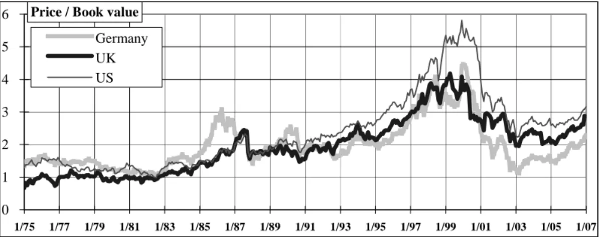
Figure 1 shows the evolution of the price/book value ratio of the British, German and United States stock markets. It can be seen that the book value, in the 90’s, has lagged considerably below the shares’ market price.
Figure 1
Evolution of the Price/Book Value Ratio on the British, German and United States Stock Mmarkets
Source: Morgan Stanley and Datastream.
0 1 2 3 4 5 6
1/75 1/77 1/79 1/81 1/83 1/85 1/87 1/89 1/91 1/93 1/95 1/97 1/99 1/01 1/03 1/05 1/07 Germany
UK US
3. Income Statement-Based Methods
Unlike the balance sheet-based methods, these methods are based on the company’s income statement. They seek to determine the company’s value through the size of its earnings, sales or other indicators. Thus, for example, it is a common practice to perform quick valuations of cement companies by multiplying their annual production capacity (or sales) in metric tons by a ratio (multiple). It is also common to value car parking lots by multiplying the number of parking spaces by a multiple and to value insurance companies by multiplying annual premiums by a multiple. This category includes the methods based on the PER: according to this method, the shares’ price is a multiple of the earnings.
The income statement for the company Alfa Inc. is shown in Table 4:
Table 4
Alfa Inc. Income Statement (Million Dollars)
Sales 300
Cost of sales 136
General expenses 120
Interest expense 4
Earnings before tax 40
Tax (35%) 14
Net income 26
3.1. Value of Earnings. PER
3According to this method, the equity’s value is obtained by multiplying the annual net income by a ratio called PER (price earnings ratio), that is:
Equity value = PER x earnings
Table 3 shows the mean PER of a number of different national stock markets in September 1992 and August 2000. Figure 2 shows the evolution of the PER for the German, English and United States stock markets.
3The PER (price earnings ratio) of a share indicates the multiple of the earnings per share that is paid on the stock market. Thus, if the earnings per share in the last year has been $3 and the share’s price is $26, its PER will be 8.66 (26/3). On other occasions, the PER takes as its reference the forecast earnings per share for the next year, or the mean earnings per share for the last few years. The PER is the benchmark used predominantly by the stock markets. Note that the PER is a parameter that relates a market item (share price) with a purely accounting item (earnings).
Figure 2
Evolution of the PER of the German, English and United States Stock Markets
Source: Morgan Stanley and Datastream.
Sometimes, the relative PER is also used, which is simply the company’s PER divided by the country’s PER.
3.2. Value of the Dividends
Dividends are the part of the earnings effectively paid out to the shareholder and, in most cases, are the only regular flow received by shareholders.4 According to this method, a share’s value is the net present value of the dividends that we expect to obtain from it. In the perpetuity case, that is, a company from which we expect constant dividends every year, this value can be expressed as follows:
Equity value = DPS / Ke
Where: DPS = dividend per share distributed by the company in the last year; Ke = required return to equity.
If, on the other hand, the dividend is expected to grow indefinitely at a constant annual rate g, the above formula becomes the following:
Equity value = DPS1 / (Ke - g) Where DPS1 is the dividends per share for the next year.
Empirical evidence5 shows that the companies that pay more dividends (as a percentage of their earnings) do not obtain a growth in their share price as a result. This is because when a company distributes more dividends, normally it reduces its growth because it distributes the money to its shareholders instead of plowing it back into new investments.
4Other flows are share buy-backs and subscription rights. However, when capital increases take place that give rise to subscription rights, the shares’ price falls by an amount approximately equal to the rights’ value.
5There is an enormous and highly varied literature about the impact of dividend policies on equity value. Some recommendable texts are to be found in Sorensen and Williamson (1985) and Miller (1986).
0 5 10 15 20 25 30 35
1/71 1/73 1/75 1/77 1/79 1/81 1/83 1/85 1/87 1/89 1/91 1/93 1/95 1/97 1/99 1/01 1/03 1/05 1/07
Germany UK US
Figure 3 shows the evolution of the dividend yield of the German, Japanese and United States stock markets.
Figure 3
Evolution of the Dividend Yield of the German, Japanese and United States Stock Markets
Source: Morgan Stanley and Datastream.
Table 3 shows the dividend yield of several international stock markets in September 1992, August 2000 and February 2007. In 2000, Japan was the country with the lowest dividend yield (0.6%) and Spain had a dividend yield of 1.5%.
3.3. Sales Multiples
This valuation method, which is used in some industries with a certain frequency, consists of calculating a company’s value by multiplying its sales by a number. For example, a pharmacy is often valued by multiplying its annual sales (in dollars) by 2 or another number, depending on the market situation. It is also a common practice to value a soft drink bottling plant by multiplying its annual sales in liters by 500 or another number, depending on the market situation.
In order to analyze this method’s consistency, Smith Barney analyzed the relationship between the price/sales ratio and the return on equity. The study was carried out in large corporations (capitalization in excess of 150 million dollars) in 22 countries. He divided the companies into five groups depending on their price/sales ratio: group 1 consisted of the companies with the lowest ratio, and group 5 contained the companies with the highest price/sales ratio. The mean return of each group of companies is shown in the following table:
Table 5
Relationship Between Return and the Price/Sales Ratio
Group 1 Group 2 Group 3 Group 4 Group 5
December 84-December 89 38.2% 36.3% 33.8% 23.8% 12.3%
December 89-September 97 10.3% 12.4% 14.3% 12.2% 9.5%
Source: Smith Barney.
0 1 2 3 4 5 6 7
1/71 1/73 1/75 1/77 1/79 1/81 1/83 1/85 1/87 1/89 1/91 1/93 1/95 1/97 1/99 1/01 1/03 1/05 1/07 Germany
Japan USA Dividend yield (%)
It can be seen from this table that, during the period December 84-December 89, the equity of the companies with the lowest price/sales ratio in December 1984 on average provided a higher return than that of the companies with a higher ratio. However, this ceased to apply during the period December 89-September 97: there was no relationship between the price/sales ratio in December 1989 and the return on equity during those years.
The price/sales ratio can be broken down into a further two ratios: Price/sales = (price/earnings) x (earnings/sales)
The first ratio (price/earnings) is the PER and the second (earnings/sales) is normally known as return on sales.
3.4. Other Multiples
In addition to the PER and the price/sales ratio, some of the frequently used multiples are:
- Value of the company / earnings before interest and taxes (EBIT).
- Value of the company / earnings before interest, taxes, depreciation and amortization
(EBITDA).
- Value of the company / operating cash flow. - Value of the equity / book value.6
Obviously, in order to value a company using multiples, multiples of comparable companies must be used.7
3.5. Multiples Used to Value Internet Companies
The multiples most commonly used to value Internet companies are Price/sales, Price/subscriber, Price/pages visited and Price/inhabitant.8
In March 2000, a French bank published its valuation of Terra based on the price/sales ratio of comparable companies:
Freeserve Tiscali Freenet.de Infosources Average
Price/Sales 110.4 55.6 109.1 21.0 74.0
Applying the mean ratio (74) to Terra’s expected sales for 2001 (310 million dollars), they estimated the value of Terra’s entire equity to be 19.105 billion dollars (68.2 dollars per share).
6
We could also list a number of other ratios which we could call “sui-generis”. One example of such ratios is the value/owner. In the initial stages of a valuation that I was commissioned to perform by a family business that was on sale, one of the brothers told me that he reckoned that the shares were worth about 30 million euros. When I asked him how he had arrived at that figure, he answered, “We are three shareholder siblings and I want each one of us to get 10 million”.
7
For a more detailed discussion of the multiples method, see Fernández (2001b). 8 See Fernández (2001a).
4. Goodwill-Based Methods
9Generally speaking, goodwill is the value that a company has above its book value or above the adjusted book value. Goodwill seeks to represent the value of the company’s intangible assets, which often do not appear on the balance sheet but which, however, contribute an advantage with respect to other companies operating in the industry (quality of the customer portfolio, industry leadership, brands, strategic alliances, etc.). The problem arises when one tries to determine its value, as there is no consensus regarding the methodology used to calculate it. Some of the methods used to value the goodwill give rise to the various valuation procedures described in this section.
These methods apply a mixed approach: on the one hand, they perform a static valuation of the company’s assets and, on the other hand, they try to quantify the value that the company will generate in the future. Basically, these methods seek to determine the company’s value by estimating the combined value of its assets plus a capital gain resulting from the value of its future earnings: they start by valuing the company’s assets and then add a quantity related with future earnings.
4.1. The “Classic” Valuation Method
This method states that a company’s value is equal to the value of its net assets (net substantial value) plus the value of its goodwill. In turn, the goodwill is valued as n times the company’s net income, or as a certain percentage of the turnover. According to this method, the formula that expresses a company’s value is:
V = A + (n x B), or V = A + (z x F)
Where: A = net asset value; n = coefficient between 1.5 and 3; B = net income; z = percentage of sales revenue; andF = turnover.
The first formula is mainly used for industrial companies, while the second is commonly used for the retail trade.
When the first method is applied to the hypothetical company Alfa Inc., assuming that the goodwill is estimated at three times the annual earnings, it would give a value for the company’s equity amounting to 213 million dollars (135 + 3 x 26).
A variant of this method consists of using the cash flow instead of the net income.
9The author feels duty bound to tell the reader that he does not like these methods at all but as they have been used a lot in the past, and they are still used from time to time, a brief description of some of them is included. However, we will not mention them again in the rest of the book. The reader can skip directly to Section 5. However, if he continues to read this section, he should not look for much “science” in the methods that follow because they are very arbitrary.
4.2. The Simplified "Abbreviated Goodwill Income" Method or the Simplified UEC
10Method
According to this method, a company’s value is expressed by the following formula: V = A + an (B - iA)
Where:
A = corrected net assets or net substantial value.
an = present value, at a rate t, of n annuities, with n between 5 and 8 years.
B = net income for the previous year or that forecast for the coming year.
i = interest rate obtained by an alternative placement, which could be debentures, the return on equities, or the return on real estate investments (after tax).
an (B - iA) = goodwill.
This formula could be explained in the following manner: the company’s value is the value of its adjusted net worth plus the value of the goodwill. The value of the goodwill is obtained by capitalizing, by application of a coefficient an, a "superprofit" that is equal to the difference
between the net income and the investment of the net assets “A” at an interest rate “i”
corresponding to the risk-free rate.
In the case of the company Alfa Inc., B = 26; A = 135. Let us assume that 5 years and 15% are used in the calculation of an, which would give an = 3.352. Let us also assume that i = 10%.
With this hypothesis, the equity’s value would be: 135 + 3.352 (26 - 0.1 x 135) = 135 + 41.9 = 176.9 million dollars.
4.3. Union of European Accounting Experts (UEC) Method
The company’s value according to this method is obtained from the following equation: V = A + an (B - iV) giving: V = [A + (an x B)] / (1 + ian)
For the UEC, a company’s total value is equal to the substantial value (or revalued net assets) plus the goodwill. This calculated by capitalizing at compound interest (using the factor an) a
superprofit which is the profit less the flow obtained by investing at a risk-free rate i a capital equal to the company’s value V.
The difference between this method and the previous method lies in the value of the goodwill, which, in this case, is calculated from the value V we are looking for, while in the simplified method, it was calculated from the net assets A.
In the case of the company Alfa Inc., B = 26; A = 135, an = 3.352, i = 10%. With these
assumptions, the equity’s value would be: (135 + 3.352 x 26) / (1 + 0.1 x 3.352) = 222.1 / 1.3352 = 166.8 million dollars.
10
4.4. Indirect Method
The formula for finding a company’s value according to this method is the following: V = (A + B/i)/2, which can also be expressed as V = A + (B - iA)/2i
The rate i used is normally the interest rate paid on long-term Treasury bonds. As can be seen in the first expression, this method gives equal weight to the value of the net assets (substantial value) and the value of the return. This method has a large number of variants that are obtained by giving different weights to the substantial value and the earnings’ capitalization value.
In the case of the company Alfa Inc., B = 26; A = 135, i = 10%. With these assumptions, the equity’s value would be 197.5 million dollars.
4.5. Anglo-Saxon or Direct Method
This method’s formula is the following: V = A + (B - iA) / tm
In this case, the value of the goodwill is obtained by restating for an indefinite duration the value of the superprofit obtained by the company. This superprofit is the difference between the net income and what would be obtained from placing at the interest rate i, a capital equal to the value of the company’s assets. The rate tm is the interest rate earned on fixed-income securities multiplied by a coefficient between 1.25 and 1.5 to adjust for the risk. In the case of the company Alfa Inc., B = 26; A = 135, i = 10%. Let us assume that tm = 15%. With these assumptions, the equity’s value would be 218.3 million dollars.
4.6. Annual Profit Purchase Method
With this method, the following valuation formula is used: V = A + m (B - iA).
Here, the value of the goodwill is equal to a certain number of years of superprofits. The buyer is prepared to pay the seller the value of the net assets plus m years of superprofits. The number of years (m) normally used ranges between 3 and 5, and the interest rate (i) is the interest rate for long-term loans.
In the case of the company Alfa Inc., B = 26; A = 135, i = 10%. With these assumptions, and if m is 5 years, the equity’s value would be 197.5 million dollars.
4.7. Risk-Bearing and Risk-Free Rate Method
This method determines a company’s value using the following expression: V = A + (B - iV) / t giving V = (A + B/t) / (1 + i/t)
The rate i is the rate of an alternative, risk-free placement; the rate t is the risk-bearing rate used to restate the superprofit and is equal to the rate i increased by a risk ratio. According to this method, a company’s value is equal to the net assets increased by the restated superprofit. As can be seen, the formula is a variant of the UEC’s method when the number of years tends towards infinity.
In the case of the company Alfa Inc., B = 26; A = 135, i = 10%. With these assumptions, if t=15%, the equity’s value would be 185 million dollars.
5. Cash Flow Discounting-Based Methods
These methods seek to determine the company’s value by estimating the cash flows it will generate in the future and then discounting them at a discount rate matched to the flows’ risk. The mixed methods described previously have been used extensively in the past. However, they are currently used increasingly less and it can be said that, nowadays, the cash flow discounting method is generally used because it is the only conceptually correct valuation method. In these methods, the company is viewed as a cash flow generator and the company’s value is obtained by calculating these flows’ present value using a suitable discount rate.
Cash flow discounting methods are based on the detailed, careful forecast, for each period, of each of the financial items related with the generation of the cash flows corresponding to the company’s operations, such as, for example, collection of sales, personnel, raw materials, administrative and sales expenses, loan repayments. Consequently, the conceptual approach is similar to that of the cash budget.
In cash flow discounting-based valuations, a suitable discount rate is determined for each type of cash flow. Determining the discount rate is one of the most important tasks and takes into account the risk, historic volatilities; in practice, the minimum discount rate is often set by the interested parties (the buyers or sellers are not prepared to invest or sell for less than a certain return, etc.).
5.1. General Method for Cash Flow Discounting
The different cash flow discounting-based methods start with the following expression:
n n n 3
3 2
2 1
k) + (1
VR CF ... k) + (1
CF k)
+ (1
CF k + 1
CF =
V + + + + +
Where: CFi = cash flow generated by the company in the period i.
Vn = residual value of the company in the year n.
k = appropriate discount rate for the cash flows’ risk.
Although at first sight it may appear that the above formula is considering a temporary duration of the flows, this is not necessarily so as the company’s residual value in the year n (Vn) can be
calculated by discounting the future flows after that period. A simplified procedure for considering an indefinite duration of future flows after the year n is to assume a constant growth rate (g) of flows after that period. Then the residual value in year n is VRn = CFn (1 + g) /
(k - g).
Although the flows may have an indefinite duration, it may be acceptable to ignore their value after a certain period, as their present value decreases progressively with longer time horizons. Furthermore, the competitive advantage of many businesses tends to disappear after a few years.
Before looking in more detail at the different cash flow discounting-based valuation methods, we must first define the different types of cash flow that can be used in a valuation.
5.2. Deciding the Appropriate Cash Flow for Discounting and the Company’s
Economic Balance Sheet
In order to understand what are the basic cash flows that can be considered in a valuation, the following chart shows the different cash streams generated by a company and the appropriate discount rates for each flow.
CASH FLOWS APPROPRIATE DISCOUNT RATE
FCF. Free cash flow WACC. Weighted average cost of capital ECF. Equity cash flow Ke. Required return to equity CFd. Debt cash flow Kd. Required return to debt
There are three basic cash flows: the free cash flow, the equity cash flow, and the debt cash flow.
The easiest one to understand is the debt cash flow, which is the sum of the interest to be paid on the debt plus principal repayments. In order to determine the present market value of the existing debt, this flow must be discounted at the required rate of return to debt (cost of the debt). In many cases, the debt’s market value shall be equivalent to its book value, which is why its book value is often taken as a sufficient approximation to the market value.11
The free cash flow (FCF) enables the company’s total value12 (debt and equity: D + E) to be obtained. The equity cash flow (ECF) enables the value of the equity to be obtained, which, combined with the value of the debt, will also enable the company’s total value to be determined. The discount rates that must be used for the FCF and the ECF are explained in the following sections.
Figure 4 shows in simplified form the difference between the company’s full balance sheet and its economic balance sheet. When we refer to the company’s (financial) assets, we are not talking about its entire assets but about total assets less spontaneous financing (suppliers, creditors...). To put it another way, the company’s (financial) assets consist of the net fixed assets plus the working capital requirements.13 The company’s (financial) liabilities consist of the shareholders’ equity (the shares) and its debt (short and long-term financial debt).14 In the rest of the paper, when we talk about the company’s value, we will be referring to the value of the debt plus the value of the shareholders’ equity (shares).
11
This is only valid if the required return to debt is equal to the debt’s cost. 12
The “company’s value” is usually considered to be the sum of the value of the equity plus the value of the financial debt.
13
For an excellent discussion of working capital requirements (WCR), see Faus (1996). 14
The shareholders’ equity or capital can include, among others, common stock, preferred stock and convertible preferred stock; and the different types of debt can include, among others, senior debt, subordinated debt, convertible debt, fixed or variable interest debt, zero or regular coupon debt, short or long-term debt, etc.
Figure 4
Full and Economic Balance Sheet of a Company
WCR = Cash + Accounts Receivable + Inventories - Accounts Payable
5.2.1. The Free Cash Flow
The free cash flow (FCF) is the operating cash flow, that is, the cash flow generated by operations, without taking into account borrowing (financial debt), after tax. It is the money that would be available in the company after covering fixed asset investments and working capital requirements, assuming that there is no debt and, therefore, there are no financial expenses.
In order to calculate future free cash flows, we must forecast the cash we will receive and must pay in each period. This is basically the approach used to draw up a cash budget. However, in company valuation, this task requires forecasting cash flows further ahead in time than is normally done in any cash budget.
Accounting cannot give us this information directly as, on one hand, it uses the accrual approach and, on the other hand, it allocates its revenues, costs and expenses using basically arbitrary mechanisms. These two features of accounting distort our perception of the appropriate approach when calculating cash flows, which must be the “cash” approach, that is, cash actually received or paid (collections and payments). However, when the accounting is adjusted to this approach, we can calculate whatever cash flow we are interested in.
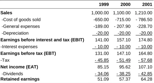
We will now try to identify the basic components of a free cash flow in the hypothetical example of the company XYZ. The information given in the accounting statements shown in Table 6 must be adjusted to give the cash flows for each period, that is, the sums of money actually received and paid in each period.
Table 6 gives the income statement for the company XYZ, SA. Using this data, we shall determine the company’s free cash flow, which we know by definition must not include any
FULL BALANCE SHEET ECONOMIC BALANCE SHEET
Assets Liabilities Assets Liabilities
Cash
Accounts
Accounts payable
receivable
Short-term Working
financial debt Capital Debt
WCR Long-term Requirements
Inventories financial debt (WCR)
Net Shareholders' Net Shareholders'
Fixed equity Fixed equity
payments to fund providers. Therefore, dividends and interest expenses must not be included in the free cash flow.
Table 7 shows how the free cash flow is obtained from earnings before interest and tax (EBIT). The tax payable on the EBIT must be calculated directly; this gives us the net income without subtracting interest payments, to which we must add the depreciation for the period because it is not a payment but merely an accounting entry. We must also consider the sums of money to be allocated to new investments in fixed assets and new working capital requirements (WCR), as these sums must be deducted in order to calculate the free cash flow.
Table 6
Income Statement for XYZ
1999 2000 2001
Sales 1,000.00 1,100.00 1,210.00
-Cost of goods sold -650.00 -715.00 - 786.50
-General expenses -189.00 - 207.90 -228.70
-Depreciation -20.00 -20.00 -20.00
Earnings before interest and tax (EBIT) 141.00 157.10 174.80
-Interest expenses - 10.00 - 10.00 - 10.00
Earnings before tax (EBT) 131.00 147.10 164.80
-Tax - 45.85 - 51.49 - 57.68
Net income (EAT) 85.15 95.62 107.10
-Dividends - 34.06 - 38.25 - 42.85
Retained earnings 51.09 57.37 64.28
Table 7
Free Cash Flow of XYZ, SA
1999 2000 2001
Earnings before interest and tax (EBIT) 141.00 157.10 174.80
-Tax paid on EBIT -49.40 -55.00 -61.20
Net income without debt 91.65 102.10 113.60
+Depreciation 20.00 20.00 20.00
- Increase in fixed assets -61.00 -67.10 -73.80
- Increase in WCR -11.00 -12.10 -13.30
Free cash flow 39.65 42.92 46.51
In order to calculate the free cash flow, we must ignore financing for the company’s operations and concentrate on the financial return on the company’s assets after tax, viewed from the perspective of a going concern, taking into account in each period the investments required for the business’s continued existence.
Finally, if the company had no debt, the free cash flow would be identical to the equity cash flow, which is another cash flow variant used in valuations and will be analyzed below.
5.2.2. The Equity Cash Flow
The equity cash flow (ECF) is calculated by subtracting from the free cash flow the interest and principal payments (after tax) made in each period to the debt holders and adding the new debt provided. In short, it is the cash flow remaining available in the company after covering fixed asset investments and working capital requirements and after paying the financial charges and repaying the corresponding part of the debt’s principal (in the event that there exists debt). This can be represented in the following expression:
ECF = FCF - [interest payments x (1- T)] - principal repayments + new debt
When making projections, the dividends and other expected payments to shareholders must match the equity cash flows.
This cash flow assumes the existence of a certain financing structure in each period, by which the interest corresponding to the existing debts is paid, the installments of the principal are paid at the corresponding maturity dates and funds from new debt are received. After that there remains a certain sum which is the cash available to the shareholders, which will be allocated to paying dividends or buying back shares.
When we restate the equity cash flow, we are valuing the company’s equity (E), and, therefore, the appropriate discount rate will be the required return to equity (Ke). To find the company’s total value (D + E), we must add the value of the existing debt (D) to the value of the equity (E). 5.2.3. Capital Cash Flow
Capital cash flow (CCF) is the term given to the sum of the debt cash flow plus the equity cash flow. The debt cash flow is composed by the sum of interest payments plus principal repayments. Therefore:
CCF = ECF + DCF = ECF + I - ∆D I = D Kd It is important to not confuse the capital cash flow with the free cash flow.
5.3. Calculating the Value of the Company Using the Free Cash Flow
In order to calculate the value of the company using this method, the free cash flows are discounted (restated) using the weighted average cost of debt and equity or weighted average cost of capital (WACC):
E + D = present value [FCF; WACC] where
D = market value of the debt. E = market value of the equity.
Kd = cost of the debt before tax = required return to debt. T = tax rate. Ke = required return to equity, which reflects the equity’s risk.
The WACC is calculated by weighting the cost of the debt (Kd) and the cost of the equity (Ke) with respect to the company’s financial structure. This is the appropriate rate for this case as, since we are valuing the company as a whole (debt plus equity), we must consider the required return to debt and the required return to equity in the proportion to which they finance the company.
WACC = E Ke + D Kd (1 - T ) E + D
5.4. Calculating the Value of the Company as the Unlevered Value Plus the
Discounted Value of the Tax Shield
In this method,15 the company’s value is calculated by adding two values: on the one hand, the value of the company assuming that the company has no debt and, on the other hand, thevalue of the tax shield obtained by the fact that the company is financed with debt.
The value of the company without debt is obtained by discounting the free cash flow, using the rate of required return to equity that would be applicable to the company if it were to be considered as having no debt. This rate (Ku) is known as the unlevered rate or required return to assets. The required return to assets is smaller than the required return to equity if the company has debt in its capital structure as, in this case, the shareholders would bear the financial risk implied by the existence of debt and would demand a higher equity risk premium. In those cases where there is no debt, the required return to equity (Ke = Ku) is equivalent to the weighted average cost of capital (WACC), as the only source of financing being used is capital.
The present value of the tax shield arises from the fact that the company is being financed with debt, and it is the specific consequence of the lower tax paid by the company as a consequence of the interest paid on the debt in each period. In order to find the present value of the tax shield, we would first have to calculate the saving obtained by this means for each of the years, multiplying the interest payable on the debt by the tax rate. Once we have obtained these flows, we will have to discount them at the rate considered appropriate. Although the discount rate to be used in this case is somewhat controversial, many authors suggest using the debt’s market cost, which need not necessarily be the interest rate at which the company has contracted its debt.
Consequently, the APV condenses into the following formula:
D + E = NPV(FCF; Ku) + value of the debt’s tax shield
5.5. Calculating the Value of the Company’s Equity by Discounting the Equity
Cash Flow
The market value of the company’s equity is obtained by discounting the equity cash flow at the rate of required return to equity for the company(Ke). When this value is added to the market value of the debt, it is possible to determine the company’s total value.
The required return to equity can be estimated using any of the following methods: 1. Gordon and Shapiro’s constant growth valuation model:
Ke = [Div1 / P0] + g. Div1 = dividends to be received in the following period = Div0(1 + g). P0 = share’s current price. g = constant, sustainable dividend growth rate.
15
This method is called APV (adjusted present value). For a more detailed discussion, the reader can see Fernández (2002, chapters 19 and 21) and Fernández (2004).
For example, if a share’s price is 200 dollars, it is expected to pay a dividend of 10 dollars and the dividend’s expected annual growth rate is 11%:
Ke = (10/200) + 0.11 = 0.16 = 16%
2. The capital asset pricing model (CAPM), which defines the required return to equity in the following terms:
Ke = RF + ß (RM - RF)
RF = rate of return for risk-free investments (Treasury bonds).
ß = share’s beta16. RM = expected market return. RM – RF = market risk premium or equity premium.
Thus, given certain values for the equity’s beta, the risk-free rate and the market risk premium, it is possible to calculate the required return to equity.17
5.6. Calculating the Company’s Value by Discounting the Capital Cash Flow
According to this model, the value of a company (market value of its equity plus market value of its debt) is equal to the present value of the capital cash flows (CCF) discounted at the weighted average cost of capital before tax (WACCBT):
E + D = present value [CCF; WACCBT]
CCF = (ECF + DCF)
There are more methods for valuing companies by discounting the expected cash flows. Fernández (2004b) explains ten different methods for Valuing Companies by Cash Flow Discounting and shows that all ten methods always give the same value. This result is logical, as all the methods analyze the same reality under the same hypotheses; they differ only in the cash flows taken as the starting point for the valuation.
5.7. Basic Stages in the Performance of a Valuation by Cash Flow Discounting
The basic stages in performing an accurate valuation by cash flow discounting are:
16The beta measures the systematic or market risk of a share. It indicates the sensitivity of the return on a share held in the company to market movements. If the company has debt, the incremental risk arising from the leverage must be added to the intrinsic systematic risk of the company’s business, thus obtaining the levered beta.
17
The classic finance textbooks provide a full discussion of the concepts analyzed here. For example, Brealey and Myers (1996), and Copeland and Weston (1988).
WACCBT = E Ke + D Kd E + D
The critical aspects in performing a company valuation are:
1. Historic and strategic analysis of the company and the industry
A. Financial analysis B. Strategic and competitive analysis Evolution of income statements and balance sheets Evolution of the industry
Evolution of cash flows generated by the company Evolution of the company’s competitive position Evolution of the company’s investments Identification of the value chain
Evolution of the company’s financing Competitive position of the main competitors Analysis of the financial health Identification of the value drivers
Analysis of the business’s risk
A. Financial forecasts B. Strategic and competitive forecasts Income statements and balance sheets Forecast of the industry’s evolution
Cash flows generated by the company Forecast of the company’s competitive position Investments Competitive position of the main competitors
Financing C. Consistency of the cash flow forecasts
Terminal value Financial consistency between forecasts Forecast of various scenarios Comparison of forecasts with historic figures
Consistency of cash flows with the strategic analysis
For each business unit and for the company as a whole
Cost of the debt, required return to equity and weighted cost of capital
Net present value of the flows at their corresponding rate. Present value of the terminal value. Value of the equity.
Benchmarking of the value obtained: comparison with similar companies Identification of the value creation. Sustainability of the value creation (time horizon)
Analysis of the value’s sensitivity to changes in the fundamental parameters Strategic and competitive justification of the value creation
2. Projections of future flows
3. Determination of the cost (required return) of capital
4. Net present value of future flows
5. Interpretation of the results
CRITICAL ASPECTS OF A VALUATION
Dynamic. The valuation is a process. The process for estimating expected risks and calibrating the risk of the different businesses and business units is crucial.
Involvement of the company. The company’s managers must be involved in the analysis of the company, of the industry and in the cash flow projections.
Multifunctional. The valuation is not a task to be performed solely by financial management. In order to obtain a good valuation, it is vital that managers from other departments take part in estimating future cash flows and their risk.
Strategic. The cash flow restatement technique is similar in all valuations, but estimating the cash flows and calibrating the risk must take into account each business unit’s strategy.
Compensation. The valuation’s quality is increased when it includes goals (sales, growth, market share, profits, investments, ...) on which the managers’ future compensation will depend.
Real options. If the company has real options, these must be valued appropriately. Real options require a totally different risk treatment from the cash flow restatements.
Historic analysis. Although the value depends on future expectations, a thorough historic analysis of the financial, strategic and competitive evolution of the different business units helps assess the forecasts’ consistency.
Technically correct. Technical correction refers basically to: a) calculation of the cash flows; b) adequate treatment of the risk, which translates into the discount rates; c) consistency of the cash flows used with the rates applied; d) treatment of the
6. Which is the Best Method to Use?
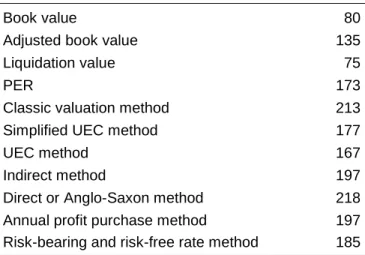
Table 8 shows the value of the equity of the company Alfa Inc. obtained by different methods based on shareholders’ equity, earnings and goodwill. The fundamental problem with these methods is that some are based solely on the balance sheet, others are based on the income statement, but none of them consider anything but historic data. We could imagine two companies with identical balance sheets and income statements but different prospects: one with high sales, earnings and margin potential, and the other in a stabilized situation with fierce competition. We would all concur in giving a higher value to the former company than to the latter, in spite of their historic balance sheets and income statements being equal.
The most suitable method for valuing a company is to discount the expected future cash flows, as the value of a company’s equity - assuming it continues to operate - arises from the company’s capacity to generate cash (flows) for the equity’s owners.
Table 8
Alfa Inc.
Value of the Equity According to Different Methods (Million Dollars)
Book value 80
Adjusted book value 135
Liquidation value 75
PER 173
Classic valuation method 213
Simplified UEC method 177
UEC method 167
Indirect method 197
Direct or Anglo-Saxon method 218
Annual profit purchase method 197
Risk-bearing and risk-free rate method 185
7. The Company as the Sum of the values of Different Divisions.
Break-up Value
On many occasions, the company’s value is calculated as the sum of the values of its different divisions or business units.18
The best way to explain this method is with an example. Table 9 shows the valuation of a North American company performed in early 1980. The company in question had three separate divisions: household products, shipbuilding, and car accessories.
18
For a more detailed discussion of this type of valuation, we recommend Chapter 14 of the book “Valuation: measuring and managing the value of companies”, by Copeland et al., edited by Wiley, 2000.
A financial group launched a takeover bid on this company at 38 dollars per share and a well-known investment bank was commissioned to value the company. This valuation, which is included in Table 9, would serve as a basis for assessing the offer.
Table 9 shows that the investment bank valued the company’s equity between 430 and 479 million dollars (or, to put it another way, between 35 and 39 dollars per share). But let us see how it arrived at that value. First of all, it projected each division’s net income and then allocated a (maximum and minimum) PER to each one. Using a simple multiplication (earnings x PER), it calculated the value of each division. The company’s value is simply the sum of the three divisions’ values.
We can call this value (between 387 and 436 million dollars) the value of the earnings generated by the company. We must now add to this figure the company’s cash surplus, which the investment bank estimated at 77.5 million dollars. However, the company’s pension plan was not fully funded (it was short by 34.5 million dollars), and consequently, this quantity had to be subtracted from the company’s value.
After performing these operations, the conclusion reached is that each share is worth between 35 and 39 dollars, which is very close to the offer made of 38 dollars per share.
Table 9
Valuation of a Company as the Sum of the Value of its Divisions Individual Valuation of Each Business Using the PER Criterion
*Cash surplus: 103.1 million dollars in cash, less 10 million dolars for operations and less 15.6 million dollars of financial debt.
8. Valuation Methods Used Depending on the Nature of the
Company
Holding companies are basically valued by their liquidation value, which is corrected to take into account taxes payable and managerial quality.
The growth of utility companies is usually fairly stable. In developed countries, the rates charged for their services are usually indexed to the CPI, or they are calculated in accordance with a legal framework. Therefore, it is simpler to extrapolate their operating statement and then discount the cash flows. In these cases, particular attention must be paid to regulatory changes, which may introduce uncertainties.
Household Car TOTAL
(Million dollars) products Shipbuilding accessories COMPANY
Expected net income 28.6 14.4 5.8 48.8
minimum maximum minimum maximum minimum maximum minimum maximum
PER for each business (minimum and maximum) 9 10 5 6 10 11
Value (million dollars) 257.4 286.0 72.0 86.4 58.0 63.8 387.4 436.2
Plus: estimated net cash surplus at year-end* 77.5 77.5
Less: non-funded retirement pensions at year-end 34.5 34.5
Value of equity (million dollars) 430.4 479.2
In the case of banks, the focus of attention is the operating profit (financial margin less commissions less operating expenses), adjusting basically for bad debts. Their industry portfolio is also analyzed. Valuations such as the PER are used, or the net worth method (shareholders’ equity adjusted for provision surpluses/deficits, and capital gains or losses on assets such as the industry portfolio).
Industrial and commercial companies. In these cases, the most commonly used valuations -apart from restated cash flows - are those based on financial ratios (PER, price/sales, price/cash flow).
These issues are discussed in greater detail in Fernández (2002, chapters 3 and 4).
9. Key Factors Affecting Value: Growth, Return, Risk and Interest
Rates
The equity’s value depends on expected future flows and the required return to equity. In turn, the growth of future flows depends on the return on investments and the company’s growth. However, the required return to equity depends on a variable over which the company has no control, the risk-free interest rate, and on the equity’s risk which, in turn, we can divide into operating risk and financial risk.
Table 10
Factors Influencing the Equity’s Value (Value Drivers)
VALUE OF EQUITY
Expectations of future cash flows Required return to equity Expected Expected Risk-free Market
return company interest risk Operating Financial
on investment growth rate premium risk risk
Compet iti ve advant age per io d A ss e ts in p la ce P ro fit m a rg in Regul at or y envi ronment Taxes Manager s. Peopl e. Cor por at e cul tur e Act ual busi ness. Bar rier s t o Adqui si tions / di sposal s Indust ry. Compet iti ve st ru ct ur e New busi nesses / pr oduct s Technol ogy Real opt ions Indust ry, count ries, la ws Cont ro l of oper at ions B u ye
r / ta
rg e t Ri sk per cei
ved by t
he mar ket Fi nanci n g Li qui di ty Si ze Ri sk management Mar ket communication
Table 10 shows that the equity’s value depends on three primary factors (value drivers):
- Expectations of future flows. - Required return to equity.
- Communication with the market.19
These factors can be subdivided in turn into return on the investment, company growth, risk-free interest rate, market risk premium, operating risk and financial risk. However, these factors are still very general. It is very important that a company identify the fundamental parameters that have most influence on the value of its shares and on value creation. Obviously, each factor’s importance will vary for the different business units.
11. Speculative Bubbles on the Stock Market
The advocates of fundamental analysis argue that share prices reflect future expectations updated by rational investors. Thus, a share’s price is equal to the net present value of all the expected future dividends. This is the so-called fundamental value. In other words, the share price reflects current earnings generation plus growth expectations. The adjective fundamental refers to the parameters that influence the share price: interest rates, growth expectations, investment’s risk...
Another group of theories is based on psychological or sociological behaviors, such as Keynes’ "animal spirits". According to these theories, share price formation does not follow any rational valuation rule but rather depends on the states of euphoria, pessimism... predominating at any given time in the financial community and in society in general. It is these psychological phenomena that give hope to the chartists: if moods do not change too often and investors value equity taking into account the share prices’ past evolution, one can expect that successive share prices will be correlated or will repeat in similar cycles.
The speculative bubble theory can be derived from fundamental analysis and occupies a middle ground between the above two theories, which seek to account for the behavior and evolution of share prices. The MIT professor Olivier Blanchard developed the algebraic expression of the speculative bubble, and it can be obtained from the same equation that gives the formula normally used by the fundamentalists. It simply makes use of the fact that the equation has several solutions, one of which is the fundamental solution and another is the fundamental solution with a speculative bubble tacked onto it. By virtue of the latter solution, a share’s price can be greater than its fundamental value (Net Present Value of all future dividends) if a bubble develops simultaneously, which at any given time may: a) continue to grow, or b) burst and vanish. To avoid tiring ourselves with equations, we can imagine the bubble as an equity overvaluation: an investor will pay today for a share a quantity that is greater than its fundamental value if he hopes to sell it tomorrow for a higher price, that is, if he hopes that the bubble will continue growing. This process can continue so long as there are investors who trust that the speculative bubble will continue to grow, that is, investors who expect to find in
19
The communication with the market factor not only refers to communication and transparency with the markets in the strict sense but also to communication with: analysts, rating companies, regulatory agencies, board of directors, employees, customers, distribution channels, partner companies, suppliers, financial institutions, and shareholders.
the future other trusting investors to whom they can sell the bubble (share) for a price that is greater than the price they have paid. Bubbles tend to grow during periods of euphoria, when it seems that the market’s only possible trend is upwards. However, there comes a day when there are no more trusting investors left and the bubble bursts and vanishes: shares return to their fundamental value.
This theory is attractive because it enables fundamental theory to be synthesized with the existence of anomalous behaviors (for the fundamentalists) in the evolution of share prices. Many analysts have used this theory to account for the tremendous drop in share prices on the New York stock market and on the other world markets on 19 October 1987. According to this explanation, the bursting of a bubble that had been growing over the previous months caused the stock market crash. A recent study performed by the Yale professor Shiller provides further evidence in support of this theory. Shiller interviewed 1000 institutional and private investors. The investors who sold before the Black Monday said that they sold because they thought that the stocks were already overvalued. However, the most surprising finding is that more than 90% of the institutional investors who did not sell said that they too believed that the market was overvalued, but hoped that they would be able to sell before the inevitable downturn. In other words, it seems that more than 90% of the institutional investors were aware that a speculative bubble was being formed - the stock was being sold for more than its fundamental value -, but trusted that they would be able to sell before the bubble burst. Among the private investors who did not sell before 19 October, more than 60% stated that they also believed that the stocks were overvalued.
Figure 5
The 1929 American Stock Market Crisis
Figure 6
The Spanish Stock Market Crisis of October 1987 0
50 100 150 200 250 300
1-26 1-27 1-28 1-29 1-30 1-31 1-32 1-33 1-34 1-35 1-36 1-37
2.000 2.200 2.400 2.600 2.800 3.000 3.200 3.400 3.600
01-87 03-87 05-87 07-87 09-87 11-87 01-88 03-88 05-88 07-88 09-88 11-88
IBEX 3
This bursting of a speculative bubble is not a new phenomenon in history. We can find recent examples in Spain in 1974 and in the USA: electronic and high-tech companies in 1962, "good concept" companies in 1970, and household name companies throughout the 70’s. In the electronic companies’ bubble, many companies’ shares in 1962 were worth less than 20% what they were worth in 1961. IBM’s share price fell from $600+ in 1961 to $300 in 1962; and Texas Instruments’ share price fell from $200+ to $50. Even larger was the bubble that grew in 1970 around the "good concept" companies: several of them lost 99% of their value in the space of just one year. Household name companies also suffered severe drops in their share prices during the 70’s: McDonald's PER fell from 83 to 9, Sony’s from 92 to 17, and Polaroid’s from 90 to 16, to give just a few examples.
Speculative bubbles can also develop outside of the stock market. One often-quoted example is that of the Dutch tulips in the 17th Century. An unusual strain of tulips began to become increasingly sought after and its price rose continuously... In the end, the tulips’ price returned to normal levels and many people were ruined. There have also been many speculative bubbles in the real estate business. The story is always the same: prices temporarily rocket upwards and then return to “normal” levels. In the process, many investors who trust that the price will continue to rise lose a lot of money. The problem with this theory, as with many of the economic interpretations, is that it provides an ingenious explanation to account for events a posteriori but it is not very useful for providing forecasts about the course that share prices will follow in the future. For this, we would need to know how to detect the bubble and predict its future course. This means being able to separate the share price into two components (the fundamental value and the bubble) and knowing the number of investors who trust that the bubble will continue to grow (here many chartists can be included). What the theory does remind us is that the bubble can burst at any time. History shows that, so far, all the bubbles have eventually burst.
The only sure recipe to avoid being trapped in a speculative bubble is to not enter it: to never buy what seems to be expensive, even if advised to do so by certain "experts", who appeal to esoteric tendencies and the foolishness or rashness of other investors.
12. Most Common Errors in Valuations
The following list contains the most common errors that the author has detected in the more than one thousand valuations he has had access to in his capacity as business consultant or professor (see Fernández and Carabias, 2006):