Signal Detection Theory Analysis of Type
1 and Type 2 Data: Meta-
d
0
,
Response-Specific Meta-
d
0
, and the Unequal
Variance SDT Model
Brian Maniscalco and Hakwan Lau
Abstract Previously we have proposed a signal detection theory (SDT) methodology for measuring metacognitive sensitivity (Maniscalco and Lau,
Conscious Cogn 21:422–430, 2012). Our SDT measure, meta-d0, provides a
response-bias free measure of how well confidence ratings track task accuracy. Here we provide an overview of standard SDT and an extended formal treatment of
meta-d0. However, whereas meta-d0 characterizes an observer’s sensitivity in tracking overall accuracy, it may sometimes be of interest to assess metacognition for a particular kind of behavioral response. For instance, in a perceptual detection task, we may wish to characterize metacognition separately for reports of stimulus presence and absence. Here we discuss the methodology for computing such a ‘‘response-specific’’ meta-d0and provide corresponding Matlab code. This approach potentially offers an alternative explanation for data that are typically taken to support the unequal variance SDT (UV-SDT) model. We demonstrate that simulated data generated from UV-SDT can be well fit by an equal variance SDT model positing different metacognitive ability for each kind of behavioral response, and likewise that data generated by the latter model can be captured by UV-SDT. This ambiguity entails that caution is needed in interpreting the processes underlying relative operating characteristic (ROC) curve properties. Type 1 ROC curves generated by combining type 1 and type 2 judgments, traditionally interpreted in
B. Maniscalco (&)
National Institute of Neurological Disorders and Stroke, National Institutes of Health, 10 Center Drive, Building 10, Room B1D728, MSC 1065, Bethesda, MD 20892-1065, USA e-mail: [email protected]
B. ManiscalcoH. Lau
Department of Psychology, Columbia University, 406 Schermerhorn Hall, 1190 Amsterdam Avenue MC 5501, New York, NY 10027, USA e-mail: [email protected]
H. Lau
Department of Psychology, UCLA, 1285 Franz Hall, Box 951563 Los Angeles, CA 90095-1563, USA
S. M. Fleming and C. D. Frith (eds.),The Cognitive Neuroscience of Metacognition, DOI: 10.1007/978-3-642-45190-4_3,Springer-Verlag Berlin Heidelberg 2014
terms of low-level processes (UV), can potentially be interpreted in terms of high-level processes instead (response-specific metacognition). Similarly, differ-ences in area under response-specific type 2 ROC curves may reflect the influence of low-level processes (UV) rather than high-level metacognitive processes.
3.1 Introduction
Signal detection theory (SDT; [10, 12]) has provided a simple yet powerful
methodology for distinguishing between sensitivity (an observer’s ability to
discriminate stimuli) and response bias (an observer’s standards for producing
different behavioral responses) in stimulus discrimination tasks. In tasks where an observer rates his confidence that his stimulus classification was correct, it may also be of interest to characterize how well the observer performs in placing these confidence ratings. For convenience, we can refer to the task of classifying stimuli as the type 1 task, and the task of rating confidence in classification accuracy as the type 2 task [2]. As with the type 1 task, SDT treatments of the type 2 task are concerned with independently characterizing an observer’s type 2 sensitivity (how well confidence ratings discriminate between an observer’s own correct and incorrect stimulus classifications) and type 2 response bias (the observer’s standards for reporting different levels of confidence).
Traditional analyses of type 2 performance investigate how well confidence ratings discriminate between all correct trials versus all incorrect trials. In addition to characterizing an observer’s overall type 2 performance in this way, it may also be of interest to characterize how well confidence ratings discriminate between correct and incorrect trials corresponding to a particular kind of type 1 response. For instance, in a visual detection task, the observer may classify the stimulus as ‘‘signal present’’ or ‘‘signal absent.’’ An overall type 2 analysis would investigate how well confidence ratings discriminate between correct and incorrect trials, regardless of whether those trials corresponded to classifications of ‘‘signal present’’ or ‘‘signal absent.’’ However, it is possible that perceptual and/or metacognitive processing qualitatively differs for ‘‘signal present’’ and ‘‘signal absent’’ trials. In light of this possibility, we may be interested to know how well confidence characterizes correct and incorrect trialsonlyfor ‘‘signal present’’ responses, oronlyfor ‘‘signal absent’’ responses (e.g. [11]). Other factors, such as experimental manipulations that target
one response type or another (e.g. [7]) may also provide impetus for such an
analysis. We will refer to the analysis of type 2 performance for correct and incorrect trials corresponding to a particular type 1 response as the analysis of
response-specific1type 2 performance.
1 We have previously used the phrase ‘‘response-conditional’’ rather than ‘‘response-specific’’
In this article, we present an overview of the SDT analysis of type 1 and type 2 performance and introduce a new SDT-based methodology for analyzing response-specific type 2 performance, building on a previously introduced method for analyzing overall type 2 performance [13]. We first provide a brief overview of type 1 SDT. We then demonstrate how the analysis of type 1 data can be extended to the type 2 task, with a discussion of how our approach compares to that of Galvin et al. [9]. We provide a more comprehensive methodological treatment of our SDT measure of type 2 sensitivity, meta-d0 [13], than has previously been published. With this foundation in place, we show how the analysis can be extended to characterize response-specific type 2 performance.
After discussing these methodological points, we provide a cautionary note on the interpretation of type 1 and type 2 relative operating characteristic (ROC) curves. We demonstrate that differences in type 2 performance for different response types can generate patterns of data that have typically been taken to support the unequal variance SDT (UV-SDT) model. Likewise, we show that the UV-SDT model can generate patterns of data that have been taken to reflect processes of a metacognitive origin. We provide a theoretical rationale for this in terms of the mathematical relationship between type 2 ROC curves and type 1 ROC curves constructed from confidence ratings, and discuss possible solutions for these difficulties in inferring psychological processes from patterns in the type 1 and type 2 ROC curves.
3.2 The SDT Model and Type 1 and Type 2 ROC Curves
3.2.1 Type 1 SDT
Suppose an observer is performing a task in which one of two possible stimulus classes (S1 or S2)2 is presented on each trial, and that following each stimulus presentation, the observer must classify that stimulus as ‘‘S1’’ or ‘‘S2.’’3We may define four possible outcomes for each trial depending on the stimulus and the observer’s response: hits, misses, false alarms, and correct rejections (Table3.1).
(Footnote 1 continued)
the type 1 and type 2 tasks. Thus, to avoid confusion, we now use ‘‘response-specific’’ to refer to type 2 performance for a given response type. We will use the analogous phrase ‘‘stimulus-specific’’ to refer to type 2 performance for correct and incorrect trials corresponding to a particular stimulus.
2 Traditionally, S1 is taken to be the ‘‘signal absent’’ stimulus andS2 the ‘‘signal present’’
stimulus. Here we follow [12] in using the more neutral terms S1 and S2 for the sake of generality.
3 We will adopt the convention of placing ‘‘S1’’ and ‘‘S2’’ in quotation marks whenever they
denote an observer’s classification of a stimulus, and omitting quotation marks when these denote the objective stimulus identity.
When an S2 stimulus is shown, the observer’s response can be either a hit (a correct classification as ‘‘S2’’) or a miss (an incorrect classification as ‘‘S1’’).
Similarly, when S1 is shown, the observer’s response can be either a correct
rejection (correct classification as ‘‘S1’’) or a false alarm (incorrect classification as ‘‘S2’’).4
A summary of the observer’s performance is provided by hit rate and false alarm rate5:
Hit Rate¼HR¼pðresp¼“S2”jstim¼S2Þ ¼nðresp¼“S2”;stim¼S2Þ
nðstim¼S2Þ
False Alarm Rate¼FAR¼pðresp¼“S2”jstim¼S1Þ ¼nðresp¼“S2”;stim¼S1Þ
nðstim¼S1Þ
wheren(C) denotes a count of the total number of trials satisfying the conditionC. ROC curves define how changes in hit rate and false alarm rate are related. For instance, an observer may become more reluctant to produce ‘‘S2’’ responses if he is informed that S2 stimuli will rarely be presented, or if he is instructed that incorrect ‘‘S2’’ responses will be penalized more heavily than incorrect ‘‘S1’’ responses (e.g. [12,22]); such manipulations would tend to lower the observer’s probability of responding ‘‘S2,’’ and thus reduce false alarm rate and hit rate. By producing multiple such manipulations that alter the observer’s propensity to respond ‘‘S2,’’ multiple (FAR, HR) pairs can be collected and used to construct the ROC curve, which plots hit rate against false alarm rate (Fig.3.1b6).
On the presumption that such manipulations affect only the observer’s
stan-dards for responding ‘‘S2,’’ and not his underlying ability to discriminate S1
stimuli from S2 stimuli, the properties of the ROC curve as a whole should be
Table 3.1 Possible outcomes for the type 1 task
Stimulus Response
‘‘S1’’ ‘‘S2’’
S1 Correct rejection (CR) False alarm (FA)
S2 Miss Hit
4 These category names are more intuitive when thinking ofS1 andS2 as ‘‘signal absent’’ and
‘‘signal present.’’ Then a hit is a successful detection of the signal, a miss is a failure to detect the signal, a correct rejection is an accurate assessment that no signal was presented, and a false alarm is a detection of a signal where none existed.
5 Since hit rate and miss rate sum to 1, miss rate does not provide any extra information beyond
that provided by hit rate and can be ignored; similarly for false alarm rate and correct rejection rate.
6 Note that the example ROC curve in Fig.3.1b is depicted as having been constructed from
confidence data (Fig.3.1a), rather than from direct experimental manipulations on the observer’s criterion for responding ‘‘S2’’. See the section titledConstructing pseudo type 1 ROC curves from type 2 databelow.
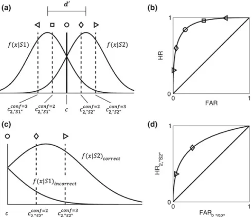
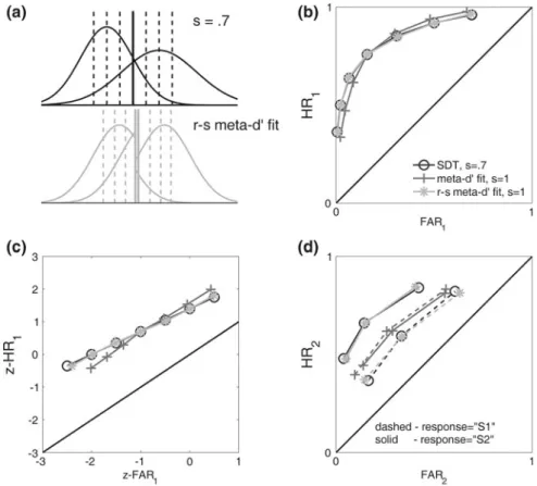
Fig. 3.1 Signal detection theory models of type 1 and type 2 ROC curves.aType 1 SDT model. On each trial, a stimulus generates an internal responsexwithin an observer, who must usexto decide whether the stimulus wasS1 orS2. For each stimulus type,xis drawn from a normal distribution. The distance between these distributions isd0, which measures the observer’s ability to discriminateS1 fromS2. The stimulus is classified as ‘‘S2’’ ifxexceeds a decision criterionc, and ‘‘S1’’ otherwise. In this example, the observer also rates decision confidence on a scale of 1–3 by comparingxto the additional response-specific type 2 criteria (dashed vertical lines).bType 1 ROC curve.d0andcdetermine false alarm rate (FAR) and hit rate (HR). By holdingd0constant and changingc, a characteristic set of (FAR, HR) points—the ROC curve—can be generated. In this example, shapes on the ROC curve mark the (FAR, HR) generated when using the corresponding criterion in panelato classify the stimulus. (Note that, because this type 1 ROC curve is generated in part by the type 2 criteria in panel 1a, it is actually a pseudo type 1 ROC curve, as discussed later in this paper.)cType 2 task for ‘‘S2’’ responses. Consider only the trials where the observer classifies the stimulus as ‘‘S2,’’ i.e. only the portion of the graph in panel a exceeding c. Then the S2 stimulus distribution corresponds to correct trials, and the S1 distribution to incorrect trials. The placement of the type 2 criteria determines the probability of high confidence for correct and incorrect trials—type 2 HR and type 2 FAR.d0 andcjointly determine to what extent correct and incorrect trials for each response type are distinguishable.
dType 2 ROC curve for ‘‘S2’’ responses. The distributions in panel c can be used to derive type 2 FAR and HR for ‘‘S2’’ responses. By holdingd0andcconstant and changingc
2,‘‘S2’’, a set of type
2 (FAR, HR) points for ‘‘S2’’ responses—a response-specific type 2 ROC curve—can be generated. In this example, shapes on the ROC curve mark the (FAR2,‘‘S2’’, HR2,‘‘S2’’) generated
informative regarding the observer’s sensitivity in discriminating S1 from S2, independent of the observer’s overallresponse biasfor producing ‘‘S2’’ responses. The observer’s sensitivity thus determines the set of possible (FAR, HR) pairs the observer can produce (i.e. the ROC curve), whereas the observer’s response bias determines which amongst those possible pairs is actually exhibited, depending on
whether the observer is conservative or liberal in responding ‘‘S2.’’ Higher
sensitivity is associated with greater area underneath the ROC curve, whereas more conservative response bias is associated with (FAR, HR) points falling more towards the lower-left portion of the ROC curve.
Measures of task performance have implied ROC curves [12,19]. An implied
ROC curve for a given measure of performance is a set of (FAR, HR) pairs that yield the same value for the measure. Thus, to the extent that empirical ROC curves dissociate sensitivity from bias, they provide an empirical target for the-oretical measures of performance to emulate. If a proposed measure of sensitivity does not have implied ROC curves that match the properties of empirical ROC curves, then this measure cannot be said to provide a bias-free measure of sensitivity.
A core empirical strength of SDT ([10, 12]; Fig. 3.1a) is that it provides a simple computational model that provides close fits to empirical ROC curves [10, 20]. According to SDT, the observer performs the task of discriminatingS1 from
S2 by evaluating internal responses along a decision axis. Every time an S1
stimulus is shown, it produces in the mind of the observer an internal response drawn from a Gaussian probability density function.S2 stimulus presentations also generate such normally distributed internal responses. For the sake of simplicity, in the following we will assume that the probability density functions forS1 andS2 have an equal standard deviationr.
The observer is able to discriminate S1 from S2 just to the extent that the
internal responses produced by these stimuli are distinguishable, such that better sensitivity for discriminating S1 from S2 is associated with larger separation between theS1 andS2 internal response distributions. The SDT measure of sen-sitivity,d0, is thus the distance between the means of theS1 andS2 distributions, measured in units of their common standard deviation:
d0¼lS2lS1
r
By convention, the internal response where theS1 andS2 distributions intersect is defined to have the value of zero, so thatlS2=rd0/2 andlS1= -rd0/2. For
simplicity, and without loss of generality, we can setr=1.
In order to classify an internal responsexon a given trial as originating from an
S1 or S2 stimulus, the observer compares the internal response to a decision
criterion, c, and only produces ‘‘S2’’ classifications for internal responses that surpass the criterion.
response¼ “S1”; xc
“S2”; x[c
Since hit rate is the probability of responding ‘‘S2’’ when an S2 stimulus is shown, it can be calculated on the SDT model as the area underneath the portion of the S2 probability density function that exceeds c. Since the cumulative distri-bution function for the normal distridistri-bution with meanland standard deviationr evaluated atxis
Uðx;l;rÞ ¼ Zx
1
1 rpffiffiffiffiffiffi2pe
ðxlÞ2
2r2
then hit rate can be derived from the parameters of the SDT model as HR¼1Uðc;lS2Þ ¼1U c;
d0
2
And similarly,
FAR¼1Uðc;lS1Þ ¼1U c;
d0
2
where omitting the r parameter in / is understood to be equivalent to setting
r=1.
By systematically altering the value of cwhile holding d0 constant, a set of (FAR, HR) pairs ranging between (0, 0) and (1, 1) can be generated, tracing out the
shape of the ROC curve (Fig.3.1b). The family of ROC curves predicted by SDT
matches well with empirical ROC curves across a range of experimental tasks and conditions [10,20].
The parameters of the SDT model can be recovered from a given (FAR, HR) pair as
d0¼zðHRÞ zðFARÞ
c¼ 0:5½zðHRÞ þzðFARÞ
wherezis the inverse of the normal cumulative distribution function. Thus, SDT analysis allows us to separately characterize an observer’s sensitivity (d0) and response bias (c) on the basis of a single (FAR, HR) pair, obviating the need to collect an entire empirical ROC curve in order to separately characterize sensi-tivity and bias—provided that the assumptions of the SDT model hold.
3.2.2 Type 2 SDT
Suppose we extend the empirical task described above, such that after classifying
the stimulus as S1 or S2, the observer must provide a confidence rating that
characterizes the likelihood of the stimulus classification being correct. This confidence rating task can be viewed as a secondary discrimination task. Just as the observer first had to discriminate whether the stimulus wasS1 orS2 by means of
providing a stimulus classification response, the observer now must discriminate whether that stimulus classification response itself was correct or incorrect by means of providing a confidence rating.7Following convention, we will refer to the task of classifying the stimulus as the ‘‘type 1’’ task, and the task of classifying the accuracy of the stimulus classification as the ‘‘type 2’’ task [2,9].
3.2.2.1 Type 2 Hit Rates and False Alarm Rates
A similar set of principles for the analysis of the type 1 task may be applied to the type 2 task. Consider the simple case where the observer rates confidence as either ‘‘high’’ or ‘‘low.’’ We can then distinguish 4 possible outcomes in the type 2 task: high confidence correct trials, low confidence correct trials, low confidence incorrect trials, and high confidence incorrect trials. By direct analogy with the type 1 analysis, we may refer to these outcomes as type 2 hits, type 2 misses, type 2 correct rejections, and type 2 false alarms, respectively (Table3.2).8
Type 2 hit rate and type 2 false alarm rate summarize an observer’s type 2 performance and may be calculated as
type 2 HR¼HR2¼pðhigh confjstim¼respÞ ¼
nðhigh conf correctÞ
nðcorrectÞ type 2 FAR¼FAR2¼pðhigh confjstim6¼respÞ ¼
nðhigh conf incorrectÞ
nðincorrectÞ Since the binary classification task we have been discussing has two kinds of correct trials (hits and correct rejections) and two kinds of incorrect trials (misses and false alarms), the classification of type 2 performance can be further
subdi-vided into a response-specific analysis, where we consider type 2 performance
only for trials where the type 1 stimulus classification response was ‘‘S1’’ or ‘‘S2’’ (Table3.3).9
7 In principle, since the observer should always choose the stimulus classification response that
is deemed most likely to be correct, then in a two-alternative task he should always judge that the chosen response is more likely to be correct than it is to be incorrect. Intuitively, then, the type 2 decision actually consists in deciding whether the type 1 response islikelyto be correct or not, where the standard for what level of confidence merits being labeled as ‘‘likely to be correct’’ is determined by a subjective criterion than can be either conservative or liberal. Nonetheless, viewing the type 2 task as a discrimination between correct and incorrect stimulus classifications facilitates comparison with the type 1 task.
8 The analogy is more intuitive when thinking of S1 as ‘‘signal absent’’ and S2 as ‘‘signal
present’’. Then the type 2 analogue of ‘‘signal absent’’ is an incorrect stimulus classification, whereas the analogue of ‘‘signal present’’ is a correct stimulus classification. The type 2 task can then be thought of as involving the detection of this type 2 ‘‘signal.’’
9 It is also possible to conduct a stimulus-specific analysis and construct stimulus-specific type 2
ROC curves. ForS1 stimuli, this would consist in a plot of p(high conf|correct rejection) vs p(high conf|false alarm). Likewise for S2 stimuli—p(high conf|hit) vs p(high conf|miss). However, as will be made clear later in the text, the present approach to analyzing type 2 ROC
Thus, when considering type 2 performance only for ‘‘S1’’ responses, HR2;“S1”¼pðhigh confjstim¼S1;resp¼“S1”Þ ¼
nðhigh conf correct rejectionÞ
nðcorrect rejectionÞ FAR2;“S1”¼pðhigh confjstim¼S2;resp¼“S1”Þ ¼
nðhigh conf missÞ
nðmissÞ
where the subscript ‘‘S1’’ indicates that these are type 2 data for type 1 ‘‘S1’’ responses.
Similarly for ‘‘S2’’ responses,
Table 3.2 Possible outcomes for the type 2 task
Accuracy Confidence
Low High
Incorrect Type 2 correct rejection Type 2 false alarm Correct Type 2 miss Type 2 hit
Table 3.3 Possible outcomes for the type 2 task, contingent on type 1 response (i.e.,
response-specific type 2 outcomes)
Response Confidence
Low High ‘‘S1’’ Accuracy Incorrect (Type 1 miss) CR2,‘‘S1’’ FA2,‘‘S1’’
Correct (Type 1 correct rejection) Miss2,‘‘S1’’ Hit2,‘‘S1’’
‘‘S2’’ Accuracy Incorrect (Type 1 false alarm) CR2,‘‘S2’’ FA2,‘‘S2’’
Correct (Type 1 hit) Miss2,‘‘S2’’ Hit2,‘‘S2’’
(Footnote 9 continued)
curves in terms of the type 1 SDT model requires each type 2 (FAR, HR) pair to be generated by the application of a type 2 criterion to two overlapping distributions. For stimulus-specific type 2 data, the corresponding type 1 model consists of only one stimulus distribution, with separate type 2 criteria for ‘‘S1’’ and ‘‘S2’’ responses generating the type 2 FAR and type 2 HR. (e.g. for theS2 stimulus, a type 2 criterion for ‘‘S1’’ responses rates confidence for type 1 misses, and a separate type 2 criterion for ‘‘S2’’ responses rates confidence for type 1 hits.) Thus there is no analogue of meta-d0for stimulus-specific type 2 data, sinced0is only defined with respect to the relationship between two stimulus distributions, whereas stimulus-specific analysis is restricted to only one stimulus distribution. It is possible that an analysis of stimulus-specific type 2 ROC curves could be conducted by positing how the type 2 criteria on either side of the type 1 criterion are coordinated, or similarly by supposing that the observer rates confidence according to an overall type 2 decision variable. For more elaboration, see the section below titled ‘‘Comparison of the current approach to that of [9].’’
HR2;“S2”¼pðhigh confjstim¼S2; resp¼“S2”Þ ¼
nðhigh conf hitÞ
nðhitÞ FAR2;“S2”¼pðhigh confjstim¼S1; resp¼“S2”Þ ¼
nðhigh conf false alarmÞ
nðfalse alarmÞ From the above definitions, it follows that overall type 2 FAR and HR are weighted averages of the response-specific type 2 FARs and HRs, where the weights are determined by the proportion of correct and incorrect trials originating from each response type:
HR2¼
nðhigh conf correctÞ
nðcorrectÞ ¼
nðhigh conf hitÞ þnðhigh conf CRÞ
nðhitÞ þnðCRÞ ¼nðhitÞ HR2;“S2”þnðCRÞ HR2;“S1”
nðhitÞ þnðCRÞ
¼pðhitjcorrectÞ HR2;“S2”þ½1pðhitjcorrectÞ HR2;“S1”
And similarly,
FAR2¼pðFAjincorrectÞ FAR2;“S2”þ½1pðFAjincorrectÞ FAR2;“S1”
Confidence rating data may be richer than a mere binary classification. In the general case, the observer may rate confidence on either a discrete or continuous
scale ranging from 1 to H. In this case, we can arbitrarily select a value h,
1\h BH, such that all confidence ratings greater than or equal tohare classified as ‘‘high confidence’’ and all others, ‘‘low confidence.’’ We can denote this choice of imposing a binary classification upon the confidence data by writing e.g.
Hconf2 ¼h, where the superscript conf=h indicates that this type 2 hit rate was calculated using a classification scheme wherehwas the smallest confidence rating considered to be ‘‘high.’’ Thus, for instance,
HR2;conf“S¼2”h ¼pðhigh confjstim¼S2; resp¼“S2”Þ ¼pðconfhjhitÞ Each choice ofhgenerates a type 2 (FAR, HR) pair, and so calculating these for
multiple values of h allows for the construction of a type 2 ROC curve with
multiple points. When using a discrete confidence rating scale ranging from 1 toH, there areH-1 ways of selectingh, allowing for the construction of a type 2 ROC
curve withH-1 points.
3.2.2.2 Adding Response-Specific Type 2 Criteria to the Type 1 SDT Model to Capture Type 2 Data
As with the type 1 task, type 2 ROC curves allow us to separately assess an observer’s sensitivity (how well confidence ratings discriminate correct from incorrect trials) and response bias (the overall propensity for reporting high
confidence) in the type 2 task. However, fitting a computational model to type 2 ROC curves is somewhat more complicated than in the type 1 case. It is not appropriate to assume that correct and incorrect trials are associated with normal probability density functions in a direct analogy to theS1 andS2 distributions of type 1 SDT. The reason for this is that specifying the parameters of the type 1 SDT model—d0andc—places strong constraints on the probability density functions for correct and incorrect trials, and these derived distributions are not normally dis-tributed [9]. In addition to this theoretical consideration, it has also been empirically demonstrated that conducting a type 2 SDT analysis that assumes normal distri-butions for correct and incorrect trials does not give a good fit to data [6].
Thus, the structure of the SDT model for type 2 performance must take into account the structure of the SDT model for type 1 performance. Galvin et al. [9] presented an approach for the SDT analysis of type 2 data based on analytically deriving formulae for the type 2 probability density functions under a suitable transformation of the type 1 decision axis. Here we present a simpler alternative approach on the basis of which response-specific type 2 ROC curves can be derived directly from the type 1 model.
In order for the type 1 SDT model to characterize type 2 data, we first need an added mechanism whereby confidence ratings can be generated. This can be accomplished by supposing that the observer simply uses additional decision criteria, analogous to the type 1 criterionc, to generate a confidence rating on the basis of the internal responsexon a given trial. In the simplest case, the observer makes a binary confidence rating—high or low—and thus needs to use two additional decision criteria to rate confidence for each kind of type 1 response. Call these response-specific type 2 criteriac2,‘‘S1’’andc2,‘‘S2’’, wherec2, ‘‘S1’’\candc2, ‘‘S2’’[c. Intuitively, confidence increases as the internal responsexbecomes more
distant from c, i.e. as the internal response becomes more likely to have been
generated by one of the two stimulus distributions.10More formally, confidenceresp¼“S1”¼
low; xc2;“S1”
high; x\c2;“S1”
confidenceresp¼“S2”¼
low; xc2;“S2”
high; x[c2;“S2”
In the more general case of a discrete confidence scale ranging from 1 to H,
thenH-1 type 2 criteria are required to rate confidence for each response type. (See e.g. Fig.3.1a, where two type 2 criteria on left/right of the type 1 criterion allow for confidence for ‘‘S1’’/‘‘S2’’ responses to be rated on a scale of 1–3.) We may define
10 See ‘‘Comparison of the current approach to that of Galvin et al. [9]’’ and footnote 12 for a
c2;“S1”¼cconf2;“S1¼2”;c2;conf“S¼31”;. . .;c2;conf“S1¼”H c2;“S2”¼ c2;conf“S¼22”;c
conf¼3 2;“S2”;. . .;c
conf¼H 2;“S2”
where e.g. c2;“S1” is a tuple containing the H-1 type 2 criteria for ‘‘S1’’ responses. Eachcconf2;“S¼1”y denotes the type 2 criterion such that internal responses more extreme (i.e. more distant from the type 1 criterion) than cconf2;“S¼1”y are asso-ciated with confidence ratings of at leasty. More specifically,
confidenceresp¼“S1”¼
1; xcconf2;“S¼21”
y; cconf2;“S¼1”yþ1x\cconf2;“S1¼”y; 1\y\H H; x\cconf¼H
2;“S1” 8
> > < > > :
confidenceresp¼“S2”¼
1; xcconf2;“S¼22”
y; cconf2;“S2¼”y\xc2;conf“S2¼”yþ1; 1\y\H H; x[cconf¼H
2;“S2” 8
> > < > > :
The type 1 and type 2 decision criteria must have a certain ordering in order for the SDT model to be meaningful. Response-specific type 2 criteria corresponding
to higher confidence ratings must be more distant from c than type 2 criteria
corresponding to lower confidence ratings. Additionally,cmust be larger than all type 2 criteria for ‘‘S1’’ responses but smaller than all type 2 criteria for ‘‘S2’’ responses. For convenience, we may define
cascending¼cconf2;“S1¼”H;c2;conf“S1¼”H1;. . .;cconf2;“S¼11”;c;cconf2;“S2¼1”;cconf2;“S2¼2”;. . .;cconf2;“S2¼”H
The ordering of decision criteria incascendingfrom first to last is the same as the ordering of the criteria from left to right when displayed on an SDT graph (e.g. Fig.3.1a). These decision criteria are properly ordered only if each element of
cascending is at least as large as the previous element, i.e. only if the Boolean
functionccascendingdefined below is true:
ccascending¼ \
2H2
i¼1
cascendingðiþ1Þ cascendingðiÞ
It will be necessary to use this function later on when discussing how to fit SDT models to type 2 data.
3.2.2.3 Calculating Response-Specific Type 2 (FAR, HR) from the Type 1 SDT Model with Response-Specific Type 2 Criteria
Now let us consider how to calculate response-specific type 2 HR and type 2 FAR from the type 1 SDT model. Recall that
HR2;conf“S2¼”h¼pðconfhjstim¼S2; resp¼“S2”Þ ¼pðconfh; hitÞ
pðhitÞ
As discussed above, p(hit), the hit rate, is the probability that an S2 stimulus
generates an internal response that exceeds the type 1 criterion c. Similarly,
p(confCh, hit), the probability of a hit endorsed with high confidence, is just the probability that an S2 stimulus generates an internal response that exceeds the high-confidence type 2 criterion for ‘‘S2’’ responses,cconf2;“S¼2”h. Thus, we can straightforwardly characterize the probabilities in the numerator and denominator of HRconf2;“S¼2”h in terms of the type 1 SDT parameters, as follows:
HRconf2;“S2¼”h¼pðconfh; hitÞ
pðhitÞ ¼
1U cconf¼h 2;“S2”;d
0
2
1U c;d0
2
By similar reasoning,
FARconf2;“S¼2”h¼
1U cconf2;“S¼2”h;d0
2
1U c;d0
2
And likewise for ‘‘S1’’ responses,
HRconf2;“S1¼”h¼U
cconf¼h 2;“S1”;d
0
2
U c;d0
2
FARconf2;“S1¼”h¼
U cconf2;“S¼1”h;d0
2
U c;d0
2
Figure3.1c illustrates how type 2 (FAR, HR) arise from type 1d0andcalong with a type 2 criterion. For instance, supposeh =3. Then the type 2 hit rate for ‘‘S2’’ responses, HRconf¼3
2;“S2”, is the probability of a high confidence hit (the area in
theS2 distribution beyondcconf2;“S¼32”) divided by the probability of a hit (the area in theS2 distribution beyondc).
By systematically altering the value of the type 2 criteria while holdingd0 and
cconstant, a set of (FAR2, HR2) pairs ranging between (0, 0) and (1, 1) can be
generated, tracing out a curvilinear prediction for the shape of the type 2 ROC
sensitivity (d0) and response bias (c) is already sufficient to determine response-specific type 2 sensitivity (i.e. the family of response-response-specific type 2 ROC curves).
3.2.3 Comparison of the Current Approach
to that of Galvin et al. [
9
]
Before continuing with our treatment of SDT analysis of type 2 data, we will make some comparisons between this approach and the one described in Galvin et al. [9].
3.2.3.1 SDT Approaches to Type 2 Performance
Galvin et al. were concerned with characterizing the overall type 2 ROC curve,
rather than response-specific type 2 ROC curves. On their modeling approach, an (FAR2, HR2) pair can be generated by setting a single type 2 criterion on a type 2
decision axis. All internal responses that exceed this type 2 criterion are labeled ‘‘high confidence,’’ and all others ‘‘low confidence.’’ By systematically changing the location of this type 2 criterion on the decision axis, the entire overall type 2 ROC curve can be traced out.
However, if the internal response x is used to make the binary confidence
decision in this way, the ensuing type 2 ROC curve behaves oddly, typically containing regions where it extends below the line of chance performance [9]. This suboptimal behavior is not surprising, in that comparing the raw value ofxto a single criterion value essentially recapitulates the decision rule used in the type 1 task and does not take into account the relationship betweenxand the observer’s type 1 criterion, which is crucial for evaluating type 1 performance. The solution is that sometransformationofxmust be used as the type 2 decision variable, ideally one that depends upon bothxandc.
For instance, consider the transformation t(x)=|x-c|. This converts the initial raw value of the internal response,x, into the distance ofxfrom the type 1 criterion. This transformed value can then plausibly be compared to a single type 2 criterion to rate confidence, e.g. an observer might rate confidence as high whenever t(x)[1. Other transformations for the type 2 decision variable are possible, and the choice is not arbitrary, since different choices for type 2 decision
variables can lead to different predictions for the type 2 ROC curve [9]. The
optimal type 2 ROC curve (i.e. the one that maximizes area under the curve) is derived by using the likelihood ratio of the type 2 probability density functions as the type 2 decision variable [9,10].
We have adopted a different approach thus far. Rather than characterizing an
overall (FAR2, HR2) pair as arising from the comparison of a single type 2
decision variable to a single type 2 criterion, we have focused on response-specific (FAR2, HR2) data arising from comparisons of the type 1 internal responsex to
separate type 2 decision criteria for ‘‘S1’’ and ‘‘S2’’ responses (e.g. Fig.3.1a). Thus, our approach would characterize the overall (FAR2, HR2) as arising from a
pair of response-specific type 2 criteria set on either side of the type 1 criterion on the type 1 decision axis, rather than from a single type 2 criterion set on a type 2 decision axis. We have posited no constraints on the setting of these type 2 criteria other than that they stand in appropriate ordinal relationships to eachother. For the sake of brevity in comparing these two approaches, in the following we will refer to Galvin et al.’s approach as G and the current approach as C.
3.2.3.2 Type 2 Decision Rules and Response-Specific Type 2 Criterion Setting
Notice that choosing a reasonable type 2 decision variable for G is equivalent to setting constraints on the relationship between type 2 criteria for ‘‘S1’’ and ‘‘S2’’
responses on C. For instance, on Gsuppose that the type 2 decision variable is
defined ast(x)=|x-c| and confidence is high ift(x)[1. On C, this is equivalent to setting response-specific type 2 criteria symmetrically about the type 1 criterion, i.e. t(c2,‘‘S1’’)=t(c2,‘‘S2’’)=|c2,‘‘S1’’ -c|=|c2,‘‘S2’’-c|=1. In other words,
assuming (on G) the general rule that confidence is high whenever the distance betweenxandcexceeds 1 requires (on C) that the type 2 criteria for each response
type both satisfy this property of being 1 unit away fromc. Any other way of
setting the type 2 criteria for C would yield outcomes inconsistent with the decision rule posited by G. Similarly, if the type 2 decision rule is that confidence is high when type 2 likelihood ratio LR2(x)[cLR2, this same rule on C would
require LR2(c2,‘‘S1’’)=LR2(c2,‘‘S2’’)=cLR2, i.e. that type 2 criteria for both
response types be set at the locations ofxon either side of ccorresponding to a type 2 likelihood ratio ofcLR2.
On G, choosing a suboptimal type 2 decision variable can lead to decreased area under the overall type 2 ROC curve. This can be understood on C as being related to the influence of response-specific type 2 criterion placement on the response-specific type 2 (FAR, HR) points, which in turn affect the overall type 2 (FAR, HR) points. As shown above, overall type 2 FAR and HR are weighted averages of the corresponding response-specific type 2 FARs and HRs. But computing a weighted average for two (FAR, HR) pairs on a concave down ROC curve will yield a new (FAR, HR) pair that lies below the original ROC curve. As a consequence, more exaggerated differences in the response-specific type 2 FAR and HR due to more exaggerated difference in response-specific type 2 criterion placement will tend to drive down the area below the overall type 2 ROC curve. Thus, the overall type 2 ROC curve may decrease even while the response-specific curves stay constant, depending on how criterion setting for each response type is coordinated. This reduced area under the overall type 2 ROC curve on C due to response-specific type 2 criterion placement is closely related to reduced area under the overall type 2 ROC curve on G due to choosing a suboptimal type 2 decision variable.
For example, consider the SDT model whered0=2,c=0,c2,‘‘S1’’ = -1, and
c2,‘‘S2’’ =1. This model yields FAR2,‘‘S1’’=FAR2,‘‘S2’’ =FAR2=0.14 and
HR2,‘‘S1’’ =HR2,‘‘S2’’=HR2=0.59. The type 1 criterion is optimally placed
and the type 2 criteria are symmetrically placed around it. This arrangement of criteria on C turns out to be equivalent to using the type 2 likelihood ratio on G, and thus yields an optimal type 2 performance. Now consider the SDT model where d0 =2, c=0, c2,‘‘S1’’= -1.5, and c2,‘‘S2’’=0.76. This model yields
FAR2,‘‘S1’’=0.04, HR2,‘‘S1’’ =0.37, FAR2,‘‘S2’’ =0.25, HR2,‘‘S2’’ =0.71, and
overall FAR2=0.14, HR2=0.54. Although d0 and c are the same as in the
previous example, now the type 2 criteria are set asymmetrically aboutc, yielding different outcomes for the type 2 FAR and HR for ‘‘S1’’ and ‘‘S2’’ responses. This has the effect of yielding a lower overall HR2 (0.54 vs. 0.59) in spite of
happening to yield the same FAR2(0.14). Thus, this asymmetric arrangement of
response-specific type 2 criteria yields worse performance on the overall type 2 ROC curve than the symmetric case for the same values ofd0andc. On G, this can be understood as being the result of choosing a suboptimal type 2 decision variable in the second example (i.e. a decision variable that is consistent with the way the response-specific type 2 criteria have been defined on C). In this case, the asymmetric placement of the response-specific type 2 criteria is inconsistent with a type 2 decision variable based on the type 2 likelihood ratio.
3.2.3.3 A Method for Assessing Overall Type 2 Sensitivity Based on the Approach of Galvin et al.
In the upcoming section, we will discuss our methodology for quantifying type 2 sensitivity with meta-d0. Meta-d0essentially provides a single measure that jointly characterizes the areas under the response-specific type 2 ROC curves for both ‘‘S1’’ and ‘‘S2’’ responses, and in this way provides a measure of overall type 2 sensitivity. However, in doing so, it treats the relationships of type 2 criteria across response types as purely a matter of criterion setting. However, as we have dis-cussed, coordination of type 2 criterion setting could also be seen as arising from the construction of a type 2 decision variable, where the choice of decision variable influences area under the overall type 2 ROC curve. We take it to be a substantive conceptual, and perhaps empirical, question as to whether it is preferable to char-acterize these effects as a matter of criterion setting (coordinating response-specific type 2 criteria) or sensitivity (constructing a type 2 decision variable). However, if one were to decide that for some purpose it were better to view this as a sensitivity effect, then the characterization of type 2 performance provided by Galvin et al. may be preferable to that of the current approach.
In the interest of recognizing this, we provide free Matlab code available online (see note at the end of the manuscript) that implements one way of using Galvin et al.’s approach to evaluate an observer’s overall type 2 performance. Given the
parameters of an SDT model, this code outputs the theoretically optimal11overall type 2 ROC curve—i.e. the overall type 2 ROC curve based on type 2 likelihood ratio, which has the maximum possible area under the curve. Maniscalco and Lau [13], building on the suggestions of Galvin et al. [9], proposed that one way of evaluating an observer’s type 2 performance is to compare her empirical type 2 ROC curve with the theoretical type 2 ROC curve, given her type 1 performance. By comparing an observer’s empirical overall type 2 ROC curve with the theo-retically optimal overall type 2 ROC curve based on type 2 likelihood ratios, the observer’s overall type 2 sensitivity can be assessed with respect to the SDT-optimal level. This approach will capture potential variation in area under the overall type 2 ROC curve that is ignored (treated as a response-specific criterion effect) by the meta-d0 approach.
3.2.3.4 Advantages of the Current Approach
Our SDT treatment of type 2 performance has certain advantages over that of Galvin et al. One advantage is that it does not require making an explicit assumption regarding what overall type 2 decision variable an observer uses, or even that the observer constructs such an overall type 2 decision variable to begin with.12This is because our approach allows the type 2 criteria for each response to vary independently, rather than positing a fixed relationship between their loca-tions. Thus, if an observer does construct an overall type 2 decision variable, our treatment will capture this implicitly by means of the relationship between the response-specific type 2 criteria; and if an observer does not use an overall type 2 decision variable to begin with, our treatment can accommodate this behavior. The question of what overall type 2 decision variables, if any, observers tend to use is a substantive empirical question, and so it is preferable to avoid making assumptions on this matter if possible.
A second, related advantage is that our approach is potentially more flexible than Galvin et al.’s in capturing the behavior of response-specific type 2 ROC curves, without loss of flexibility in capturing the overall type 2 ROC curve. (Since overall type 2 ROC curves depend on the response-specific curves, as shown above, our focus on characterizing the response-specific curves does not entail a deficit in capturing the overall curve.) A third advantage is that our approach provides a simple way to derive response-specific type 2 ROC curves from the
11 Provided the assumptions of the SDT model are correct.
12 Of course, our approach must at least implicitly assume a type 2 decision variablewithineach
response type. In our treatment, the implicit type 2 decision variable for each response type is just the distance ofxfromc. However, for the analysis of response-specific type 2 performance for the equal variance SDT model, distance from criterion and type 2 likelihood ratio are equivalent decision variables. This is because they vary monotonically with each other [9], and so produce the same type 2 ROC curve [5,21].
type 1 SDT model, whereas deriving the overall type 2 ROC curve is more complex under Galvin et al.’s approach and depends upon the type 2 decision variable being assumed.
3.3 Characterizing Type 2 Sensitivity in Terms
of Type 1 SDT: Meta-
d
0Since response-specific type 2 ROC curves can be derived directly fromd0andcon the SDT model, this entails a tight theoretical relationship between type 1 and type 2 performance. One practical consequence is that type 2 sensitivity—the empirical type 2 ROC curves—can be quantified in terms of the type 1 SDT parametersd0and
c[13]. However, it is necessary to explicitly differentiate instances whend0is meant to characterize type 1 performance from those instances whend0(along withc) is meant to characterize type 2 performance. Here we adopt the convention of using the variable names meta-d0and meta-cto refer to type 1 SDT parameters when used to characterize type 2 performance. We will refer to the type 1 SDT model as a whole, when used to characterize type 2 performance, as the meta-SDT model. Essentially,d0andcdescribe the type 1 SDT model fit to the type 1 ROC curve,13
whereas meta-d0 and meta-c—the meta-SDT model—quantify the type 1 SDT
model when used exclusively to fit type 2 ROC curves.
How do we go about using the type 1 SDT model to quantify type 2 performance? There are several choices to make before a concrete method can be proposed. In the course of discussing these issues, we will put forth the methodological approach originally proposed by Maniscalco and Lau [13].
3.3.1 Which Type 2 ROC Curves?
As discussed in the preceding section ‘‘Comparison of the current approach to that of Galvin et al. [9],’’ we find the meta-SDT fit that provides the best simultaneous fit to the response-specific type 2 ROC curves for ‘‘S1’’ and ‘‘S2’’ responses, rather than finding a model that directly fits the overall type 2 ROC curve. As explained in more detail in that prior discussion, we make this selection primarily because (1) it allows more flexibility and accuracy in fitting the overall data set, and (2) it does not require making an explicit assumption regarding what type 2 decision variable the observer might use for confidence rating.
13 When the multiple points on the type 1 ROC curve are obtained using confidence rating data,
it is arguably preferable to calculated0andconly from the (FAR, HR) pair generated purely by the observer’s type 1 response. The remaining type 1 ROC points incorporate confidence rating data and depend on type 2 sensitivity, and so estimatingd0on the basis of these ROC points may confound type 1 and type 2 sensitivity. See the section below titled ‘‘Response-specific meta-d0 and the unequal variance SDT model’’.
3.3.2 Which Way of Using Meta-
d
0and Meta-c to Derive
Response-Specific Type 2 ROC Curves?
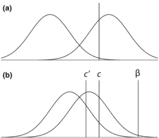
A second consideration is how to characterize the response-specific type 2 ROC curves using meta-d0and meta-c. For the sake of simplifying the analysis, and for the sake of facilitating comparison betweend0and meta-d0, an appealing option is toa priorifix the value of meta-cso as to be similar to the empirically observed type 1 response bias c, thus effectively allowing meta-d0 to be the sole free parameter that characterizes type 2 sensitivity. However, since there are multiple ways of measuring type 1 response bias [12], there are also multiple ways of fixing the value of meta-con the basis ofc. In addition to the already-introducedc, type 1 response bias can be measured with the relative criterion,c0:
c0¼c=d0
This measure takes into account how extreme the criterion is, relative to the
stimulus distributions.
Bias can also be measured asb,the ratio of the probability density function for
S2 stimuli to that ofS1 stimuli at the location of the decision criterion:
b¼ecd0
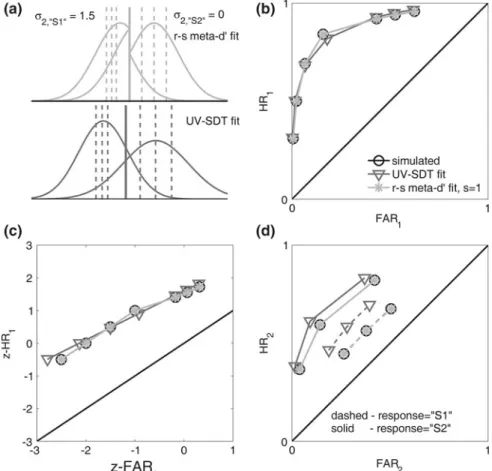
Figure3.2shows an example of howc,c0, andb relate to the stimulus distri-butions when bias is fixed andd0varies. Panel a shows an SDT diagram ford0=3
and c=1. In panel b, d0 =1 and the three decision criteria are generated by
settingc,c0, andbto the equivalent values of those exhibited by these measures in panel a. Arguably,c0performs best in terms of achieving a similar ‘‘cut’’ between the stimulus distributions in panels a and b. This is an intuitive result given thatc0
essentially adjusts the location of c according to d0. Thus, holding c0 constant ensures that, as d0 changes, the location of the decision criterion remains in a similar location with respect to the means of the two stimulus distributions.
By choosingc0as the measure of response bias that will be held constant in the estimation of meta-d0, we can say that when the SDT and meta-SDT models are fit to the same data set, they will have similar type 1 response bias, in the sense that they have the samec0value. This in turn allows us to interpret a subject’s meta-d0
in the following way: ‘‘Suppose there is an ideal subject whose behavior is per-fectly described by SDT, and who performs this task with a similar level of response bias (i.e. samec0) as the actual subject. Then in order for our ideal subject to produce the actual subject’s response-specific type 2 ROC curves, she would need herd0to be equal to meta-d0.’’
Thus, meta-d0can be found by fitting the type 1 SDT model to response-specific type 2 ROC curves, with the constraint that meta-c0=c0. (Note that in the below we list meta-c, rather than meta-c0,as a parameter of the meta-SDT model. The constraint meta-c0=c0can thus be satisfied by ensuring meta-c=meta-d0 9c0.)
3.3.3 What Computational Method of Fitting?
If the response-specific type 2 ROC curves contain more than one empirical (FAR2, HR2) pair, then in general an exact fit of the model to the data is not
possible. In this case, fitting the model to the data requires minimizing some loss function, or maximizing some metric of goodness of fit.
Here we consider the procedure for finding the parameters of the type 1 SDT model that maximize the likelihood of the response-specific type 2 data. Maximum likelihood approaches for fitting SDT models to type 1 ROC curves with multiple data points have been established [4, 16]. Here we adapt these existing type 1 approaches to the type 2 case. The likelihood of the type 2 data can be charac-terized using the multinomial model as
Ltype2ðhjdataÞ / Y y;s;r
Probhðconf¼yjstim¼s; resp¼rÞndataðconf¼yjstim¼s;resp¼rÞ
Maximizing likelihood is equivalent to maximizing log-likelihood, and in practice it is typically more convenient to work with likelihoods. The log-likelihood for type 2 data is given by
log Ltype2ðhjdataÞ / X y;s;r
ndatalog Probh
Fig. 3.2 Example behavior of holding response bias constant asd0changes forc,c0, andb.aAn
SDT graph whered0=3 andc=1. The criterion location can also be quantified asc0 =c/d0=1/3 and logb=c9d0 =3.bAn SDT graph whered0=1. The three decision criteria plotted here represent the locations of the criteria that preserve the value of the corresponding response bias exhibited in panel a. So e.g. the criterion markedc0in panel b has the same value ofc0as the criterion in panel a (=1/3), and likewise forc(constant value of 1) andb(constant value of 3)
his the set of parameters for the meta-SDT model:
h¼ meta-d0;meta-c;meta-c2;“S1”;meta-c2;“S2”
ndataðconf¼yjstim¼s; resp¼rÞis a count of the number of times in the data a confidence rating ofywas provided when the stimulus wassand response wasr.
y,s, andrare indices ranging over all possible confidence ratings, stimulus classes, and stimulus classification responses, respectively.
probhðconf¼yjstim¼s; resp¼rÞ is the model-predicted probability of gen-erating confidence ratingyfor trials where the stimulus and response weresandr, given the parameter values specified inh.
Calculation of these type 2 probabilities from the type 1 SDT model is similar to the procedure used to calculate the response-specific type 2 FAR and HR. For notational convenience, below we express these probabilities in terms of the standard SDT model parameters, omitting the ‘‘meta’’ prefix.
For convenience, define
_
c2;“S1”¼c;c2;conf“S1¼2”;c2;conf“S¼31”;. . .;cconf2;“S1¼”H;1
_
c2;“S2”¼c;c2;conf“S2¼2”;c2;conf“S¼32”;. . .;cconf2;“S2¼”H;1 Then
Prob confð ¼yjstim¼S1; resp¼“S1”Þ ¼U c_2;“S1”ðyÞ;
d0
2
U c_2;“S1”ðyþ1Þ;d0
2
U c;d0
2
Prob confð ¼yjstim¼S1;resp¼“S2”Þ ¼U c_2;“S2”ðyþ1Þ;
d0
2
U c_2;“S2”ð Þy;d0
2
1U c;d0
2
Prob confð ¼yjstim¼S2; resp¼“S2”Þ ¼U c_2;“S2”ðyþ1Þ;
d0 2
U c_2;“S2”ð Þy;d0 2
1U c;d0
2
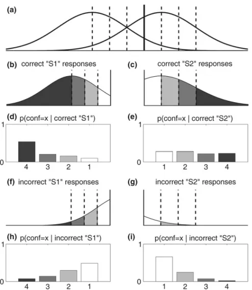
An illustration of how these type 2 probabilities are derived from the type 1 SDT model is provided in Fig.3.3.
The multinomial model used as the basis for calculating likelihood treats each discrete type 2 outcome (conf=y| stim=s, resp=r) as an event with a fixed probability that occurred a certain number of times in the data set, where outcomes across trials are assumed to be statistically independent. The probability of the entire set of type 2 outcomes across all trials is then proportional to the product of the probability of each individual type 2 outcome, just as e.g. the probability of
Fig. 3.3 Type 2 response probabilities from the SDT model.aAn SDT graph withd0=2 and decision criteriac=0.5,c2,‘‘S1’’=(0,-0.5,-1), andc2,‘‘S2’’=(1, 1.5, 2). The type 1 criterion
(solid vertical line) is set to the value of 0.5, corresponding to a conservative bias for providing ‘‘S2’’ responses, in order to create an asymmetry between ‘‘S1’’ and ‘‘S2’’ responses for the sake of illustration. Seven decision criteria are used in all, segmenting the decision axis into 8 regions. Each region corresponds to one of the possible permutations of type 1 and type 2 responses, as there are two possible stimulus classifications and four possible confidence ratings.b–iDeriving probability of confidence rating contingent on type 1 response and accuracy. How would the SDT model depicted in panel (a) predict the probability of each confidence rating for correct ‘‘S1’’ responses? Since we wish to characterize ‘‘S1’’ responses, we need consider only the portion of the SDT graph falling to the left of the type 1 criterion. Since ‘‘S1’’ responses are only correct when theS1 stimulus was actually presented, we can further limit our consideration to internal responses generated byS1 stimuli. This is depicted in panel (b). This distribution is further subdivided into 4 levels of confidence by the 3 type 2 criteria (dashed vertical lines), where darker regions correspond to higher confidence. The area under theS1 curve in each of these
throwing 4 heads and 6 tails for a fair coin is proportional to 0.5490.56. (Calculation of the exact probability depends on a combinatorial term which is
invariant with respect to h and can therefore be ignored for the purposes of
maximum likelihood fitting.)
Likelihood,L(h), can be thought of as measuring how probable the empirical data is, according to the model parameterized withh. A very lowL(h) indicates
that the model with h would be very unlikely to generate a pattern like that
observed in the data. A higherL(h) indicates that the data are more in line with the typical behavior of data produced by the model withh. Mathematical optimization techniques can be used to find the values ofhthat maximize the likelihood, i.e. that create maximal concordance between the empirical distribution of outcomes and the model-expected distribution of outcomes.
The preceding approach for quantifying type 2 sensitivity with the type 1 SDT model—i.e. for fitting the meta-SDT model—can be summarized as a mathe-matical optimization problem:
h¼argmax
h
Ltype2ðhjdataÞ; subject to: meta-c0¼c0;c meta-cascending
where type 2 sensitivity is quantified by meta-d02h.
cmeta-cascendingis the Boolean function described previously, which returns a value of ‘‘true’’ only if the type 1 and type 2 criteria stand in appropriate ordinal relationships.
We provide free Matlab code, available online, for implementing this maximum likelihood procedure for fitting the meta-SDT model to a data set (see note at the end of the manuscript).
3.3.4 Toy Example of Meta-
d
0Fitting
An illustration of the meta-d0 fitting procedure is demonstrated in Fig.3.4using simulated data. In this simulation, we make the usual SDT assumption that on each trial, presentation of stimulus S generates an internal responsexthat is drawn from the probability density function of S, and that a type 1 response is made by comparingxto the decision criterionc. However, we now add an extra mechanism to the model to allow for the possibility of added noise in the type 2 task. Let us call the internal response used to rate confidence x2. The type 1 SDT model we regions, divided by the total area under theS1 curve that falls below the type 1 criterion, yields the probability of reporting each confidence level, given that the observer provided a correct ‘‘S1’’ response. Panel (d) shows these probabilities as derived from areas under the curve in panel (b). The remaining panels display the analogous logic for deriving confidence probabilities for incorrect ‘‘S1’’ responses (f,h), correct ‘‘S2’’ responses (c,e), and incorrect ‘‘S2’’ responses (g,i)
have thus far considered assumesx2=x. In this example, we suppose thatx2is a
noisier facsimile ofx. Formally,
x2¼xþn; n Nð0;r2Þ
whereN(0,r2) is the normal distribution with mean 0 and standard deviationr2.
The parameterr2thus determines how much noisierx2is thanx. Forr2=0 we
expect meta-d0=d0, and forr2[0 we expect meta-d0\d0.
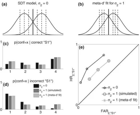
Fig. 3.4 Fitting meta-d0 to response-specific type 2 data.a Graph for the SDT model where
d0=2 andr2=0 (see text for details).bA model identical to that in panel a, with the exception
that r2=1, was used to create simulated data. This panel displays the SDT graph of the
parameters for the meta-d0fit to ther2=1 data.c,dResponse-specific type 2 probabilities. The
maximum likelihood method of fitting meta-d0 to type 2 data uses response-specific type 2 probabilities as the fundamental unit of analysis. The type 1 SDT parameters that maximize the likelihood of the type 2 data yield distributions of response-specific type 2 probabilities closely approximating the empirical (here, simulated) distributions. Here we only show the probabilities for ‘‘S1’’ responses; because of the symmetry of the generating model, ‘‘S2’’ responses follow identical distributions.eResponse-specific type 2 ROC curves. ROC curves provide a more informative visualization of the type 2 data than the raw probabilities. Here it is evident that there is considerably less area under the type 2 ROC curve for ther2=1 simulation than is predicted
The simulated observer rates confidence on a 4-point scale by comparingx2to response-specific type 2 criteria, using the previously defined decision rules for
confidence in the type 1 SDT model.14
We first considered the SDT model withd0 =2,c=0,c2,‘‘S1’’=(-0.5, -1,
-1.5),c2,‘‘S2’’ =(0.5, 1, 1.5) andr2=0. Becauser2=0, this is equivalent to the
standard type 1 SDT model. The SDT graph for these parameter values is plotted in Fig.3.4a. Using these parameter settings, we computed the theoretical proba-bility of each confidence rating for each permutation of stimulus and response.
These probabilities for ‘‘S1’’ responses are shown in panels c and d, and the
corresponding type 2 ROC curve is shown in panel e. (Because the type 1 criterion
cis unbiased and the type 2 criteria are set symmetrically aboutc, confidence data for ‘‘S2’’ responses follow an identical distribution to that of ‘‘S1’’ responses and are not shown.)
Next we simulated 10,000,000 trials using the same parameter values as the previously considered model, with the exception thatr2=1. With this additional
noise in the type 2 task, type 2 sensitivity should decrease. This decrease in type 2 sensitivity can be seen in the type 2 ROC curve in panel e. There is more area
underneath the type 2 ROC curve whenr2=0 than whenr2=1.
We performed a maximum likelihood fit of meta-d0to the simulated type 2 data using the fmincon function in the optimization toolbox for Matlab (MathWorks, Natick, MA), yielding a fit with parameter values meta-d0 =1.07, meta-c=0, meta-c2,‘‘S1’’=(-0.51,-0.77,-1.06), and meta-c2,‘‘S2’’=(0.51, 0.77, 1.06). The
SDT graph for these parameter values is plotted in Fig.3.4b.
Panels c and d demonstrate the component type 2 probabilities used for com-puting the type 2 likelihood. The response-specific type 2 probabilities forr2=0
are not distributed the same way as those forr2=1, reflecting the influence of
adding noise to the internal response for the type 2 task. Computing meta-d0for the r2=1 data consists in finding the parameter values of the ordinary type 1 SDT
model that maximize the likelihood of ther2=1 response-specific type 2 data.
This results in a type 1 SDT model whose theoretical type 2 probabilities closely
14 Note that for this model, it is possible forxandx
2to be on opposite sides of the type 1
decision criterionc(see, e.g. Fig.3.5a, b). This is not problematic, since onlyxis used to provide the type 1 stimulus classification. It is also possible forx2to surpass some of the type 2 criteria on
the opposite side of c. For instance, suppose that x= -0.5, x2=+0.6, c=0, and cconf¼h
2;“S2” ¼ þ0:5. Thenxis classified as anS1 stimulus, and yetx2surpasses the criterion for rating ‘‘S2’’ responses with a confidence ofh. Thus, there is potential for the paradoxical result whereby the type 1 response is ‘‘S1’’ and yet the type 2 confidence rating is rated highly due to the relatively strong ‘‘S2’’-ness ofx2. In this example, the paradox is resolved by the definition of the type 2 decision rules stated above, which stipulate that internal responses are only evaluated with respect to the response-specific type 2 criteria that are congruent with the type 1 response. Thus, in this case, the decision rule would not comparex2with the type 2 criteria for ‘‘S2’’ responses to begin with. Instead, it would find that x2does not surpass the minimal confidence criterion for ‘‘S1’’ responses (i.e.,x2[c[cconf2;“S1¼”2) and would therefore assignx2a confidence of 1. Thus, in this case, the paradoxical outcome is averted. But such potentially paradoxical results need to be taken into account for any SDT model that posits a potential dissociation betweenxandx2.
match the empirical type 2 probabilities for the simulatedr2=1 data (Fig.3.4c, d).
Because type 2 ROC curves are closely related to these type 2 probabilities, the
meta-d0 fit also produces a type 2 ROC curve closely resembling the simulated
curve, as shown in panel e.
3.3.5 Interpretation of Meta-
d
0Notice that because meta-d0characterizes type 2 sensitivity purely in terms of the type 1 SDT model, it does not explicitly posit any mechanisms by means of which type 2 sensitivity varies. Although the meta-d0fitting procedure gave a good fit to data simulated by the toyr2model discussed above, it could also produce
simi-larly good fits to data generated by different models that posit completely different
mechanisms for variation in type 2 performance. In this sense, meta-d0 is
descriptive but not explanatory. It describes how an ideal SDT observer with similar type 1 response bias as the actual subject would have achieved the observed type 2 performance, rather than explain how the actual subject achieved their type 2 performance.
The primary virtue of using meta-d0is that it allows us to quantify type 2 sen-sitivity in a principled SDT framework, and compare this against SDT expectations of what type 2 performanceshould have been, given performance on the type 1 task, all while remaining agnostic about the underlying processes. For instance, if we find that a subject has d0 =2 and meta-d0=1, then (1) we have taken appropriate SDT-inspired measures to factor out the influence of response bias in our measure of type 2 sensitivity; (2) we have discovered a violation of the SDT expectation that meta-d0=d0 =2, giving us a point of reference in interpreting the subject’s metacognitive performance in relation to their primary task performance and suggesting that the subject’s metacognition is suboptimal (provided the assumptions of the SDT model hold); and (3) we have done so while making minimal assump-tions and commitments regarding the underlying processes.
Another important point for interpretation concerns the raw meta-d0 value, as opposed to its value in relation tod0. Suppose observers A and B both have
meta-d0 =1, but d0A=1 and d0B=2. Then there is a sense in which they have
equivalent metacognition, as their confidence ratings are equally sensitive in discerning correct from incorrect trials. But there is also a sense in which A has superior metacognition, since A was able to achieve the same level of meta-d0as B in spite of a lowerd0. In a sense, A is more metacognitively ideal, according to SDT. We can refer to the first kind of metacognition, which depends only on
meta-d0, as ‘‘absolute type 2 sensitivity,’’ and the second kind, which depends on the relationship between meta-d0andd0, as ‘‘relative type 2 sensitivity.’’ Absolute and relative type 2 sensitivity are distinct constructs that inform us about distinct aspects of metacognitive performance.
3.4 Response-Specific Meta-
d
0Thus far we have considered how to characterize an observer’s overall type 2 sensitivity using meta-d0, expounding upon the method originally introduced in
Maniscalco and Lau [13]. Here we show how to extend this analysis and
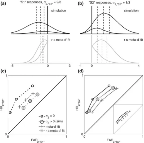
char-acterize response-specific type 2 sensitivity in terms of the type 1 SDT model. In the below we focus on ‘‘S1’’ responses, but similar considerations apply for ‘‘S2’’ responses.
We wish to find the type 1 SDT parametershthat provide the best fit to the type 2 ROC curve for ‘‘S1’’ responses, i.e. the set of empiricalFARconf2;“S1¼”h;HRconf2;“S¼1”h
for all h satisfying 2BhBH. Thus, we wish to find the h that maximizes the
likelihood of the type 2 probabilities for ‘‘S1’’ responses, using the usual meta-d0
fitting approach. This is essentially equivalent to applying the original meta-d0
procedure described above to the subset of the model and data pertaining to ‘‘S1’’ responses.
Thus, we wish to solve the optimization problem
h“S1” ¼argmax
h“S1”
L2;“S1”ðh“S1”jdataÞ;
subject to: meta-c0“S1”¼c0; cmeta-cascending
where
h“S1”¼ meta-d“0S1”;meta-c“S1”;meta-c2;“S1”
L2;“S1”ðh“S1”jdataÞ /
Y y;s
Probhðconf¼yjstim¼s;resp¼“S1”Þndataðconf¼yjstim¼s;resp¼“S1”Þ
meta-d0“S1”2h“S1” measures type 2 sensitivity for ‘‘S1’’ responses.
The differences between this approach and the ‘‘overall’’ meta-d0 fit are
straightforward. The same likelihood function is used, but with the indexrfixed to the value ‘‘S1’’.h“S1”is equivalent tohexcept for its omission of metac2;“S2”, since
type 2 criteria for ‘‘S2’’ responses are irrelevant for fitting ‘‘S1’’ type 2 ROC curves. The type 1 criterion meta-c‘‘S1’’ is listed with a ‘‘S1’’ subscript to distin-guish it from meta-c‘‘S2’’, the type 1 criterion value from the maximum likelihood
fit to ‘‘S2’’ type 2 data. Since the maximum likelihood fitting procedure enforces the constraint meta-c0‘‘S1’’=c0, it follows that meta-c‘‘S1’’=meta-d0‘‘S1’’ 9c0.
Thus, in the general case where meta-d0‘‘S1’’ =meta-d0‘‘S2’’ andc0=0, it is also
true that meta-c‘‘S1’’=meta-c‘‘S2’’.
We provide free Matlab code, available online, for implementing this maximum likelihood procedure for fitting the response-specific meta-SDT model to a data set (see note at the end of the manuscript).