Abstract—This paper presents experimental and analytical
results of an investigation of the three major cutting parameters—cutting speed, feed rate, and depth of cut—that affect the surface finish of turned parts in dry turning. A two-level, three-parameter experiment was planned using design-of-experiment methodology. The selected work materials were aluminium (AISI 6061), mild steel (AISI 1030), and alloy steel (AISI 4340). The results were analysed applying three methods—traditional analysis, Pareto ANOVA, and the Taguchi method. Subsequently, predictive models were developed for each material applying regression analysis. The results indicate that, while the feed rate has a dominant effect on surface finish, the interaction between cutting speed and feed rate also plays a major role which is influenced by the properties of work material.
Index Terms—Cutting parameters, dry turning, Pareto
ANOVA analysis, regression analysis, Taguchi method
I. INTRODUCTION
URFACE finish of the machined parts is one of the important criteria by which the success of a machining operation is judged [1]. It is also an important quality characteristic that may dominate the functional requirements of many component parts. For example, good surface finish is necessary to prevent premature fatigue failure; to improve corrosion resistance; to reduce friction, wear, and noise; and finally to improve product life. Therefore, achieving the required surface finish is critical to the success of many machining operations.
Over the years, cutting fluids have been applied extensively in machining operations for various reasons, such as to reduce friction and wear, hence improving tool life and surface finish; to reduce force and energy consumption; and to cool the cutting zone, thus reducing thermal distortion of the workpiece and improving tool life, and facilitating chip disposal. However, the application of cutting fluid poses serious health and environmental hazards. Operators exposed to cutting fluids may have various health problems. If not disposed of properly, cutting fluids may adversely affect the environment and carry economic consequences.
To overcome these problems a number of techniques, such
Manuscript received February 22, 2011.
M. N. Islam is a senior lecturer at the department of Mechanical Engineering, Curtin University, GPO Box U1987, Perth, WA 6845, Australia (e-mail: M.N.Islam@ curtin.edu.au).
Brian Boswell is a lecturer at the department of Mechanical Engineering, Curtin University, GPO Box U1987, Perth, WA 6845, Australia (phone: +618 9266 3803; fax +618 9266 2681; e-mail: B.Boswell@ curtin.edu.au).
as dry turning, turning with minimum quantity lubrication (MQL), and cryogenic turning have been proposed. Dry turning is characterised by the absence of any cutting fluid, and unlike MQL and cryogenic turning does not require any additional delivery system. Hence, from the environmental perspective, dry turning is ecologically desirable; and from an economic perspective, it decreases manufacturing costs by 16 to 20% [2]. Nevertheless, in spite of all economic and environmental benefits, the quality of the component parts produced by dry turning should not be sacrificed.
The two major functions of cutting fluids are (i) to increase tool life and (ii) to improve the surface finish of manufactured parts. However, with the advent of various new tool materials and their deposition techniques, the tool lives of modern tools have increased significantly. At present, dry machining is possible without considerable tool wear; as such, research work has been focused on the surface finish aspect of dry turning.
Investigations of the surface finish of turned parts have received notable attention in the literature, but most of the reported studies concentrate on a single work material such as free machining steel [3], composite material [4], bearing steel [5], SCM 400 steel [6], tool steel [7], MDN250 steel [8], and alloy steel [9]. However, the work material has significant effects on the results of machining operations. Therefore, any study on machining operations would not be complete unless it covered a wide range of materials. Consequently, three work materials encompassing diverse machinability ratings were selected for this study.
II. SCOPE
Several factors directly or indirectly influence the surface finish of machined parts, such as cutting conditions, tool geometry, work material, machine accuracy, chatter or vibration of the machine tool, cutting fluid, and chip formation. The objective of this research was to investigate the effects of major input parameters on the surface finish of parts produced by dry turning, and to optimise the input parameters. From a user’s point of view, cutting parameters—cutting speed, feed rate, and depth of cut—are the three major controllable variables; as such they were selected as input parameters.
Surface roughness represents the random and repetitive
deviations of a surface profile from the nominal surface. It can be expressed by a number of parameters such as arithmetic average, peak-to-valley height, and ten-point height. Yet, no single parameter appears to be capable of describing the surface quality adequately. In this study,
An Investigation of Surface Finish in Dry
Turning
M. N. Islam,
Member, IAENG
and Brian Boswell
arithmetic average has been adopted to represent surface
roughness, as it is the most frequently used and internationally accepted parameter. The arithmetic average represents the average of the absolute deviations from the mean surface level which can be calculated using the following formula:
dx
x
Y
L
R
L
a
=
∫
0
)
(
1
(1) where Ra is the arithmetic average roughness, Y is the
vertical deviation from the nominal surface, and L is the
specified distanced over which the surface roughness is measured [10]. For this research, a surface finish analyser capable of measuring multiple surface finish parameters was employed. The results were then analysed by three techniques—traditional analysis, Pareto ANOVA analysis, and Taguchi’s signal-to-noise ratio (S/N) analysis.
In the traditional analysis, the average values of the measured variables were used. This tool is particularly suitable for monitoring a trend of change in the relationship of variables.
Pareto ANOVA analysis is an excellent tool for determining the contribution of each input parameter and their interactions with the output parameters (surface roughness). It is a simplified ANOVA analysis method that does not require an ANOVA table. Further details on Pareto ANOVA can be found in Park [11].
The Taguchi method applies the signal-to-noise ratio to
optimise the outcome of a manufacturing process. The signal-to-noise ratio can be calculated using the following formula:
−
=
∑
= n
i i
y
n
N
S
1 2
1
log
10
(2)where S/N is the signal-to-noise ratio (in dB), n is the
number of observations, and y is the observed data.
The above formula is suitable for quality characteristics in which the adage ‘the smaller the better’ holds true, which is the case for surface roughness. The higher the value of the S/N ratio, the better the result is because it guarantees optimum quality with minimum variance. A thorough treatment of the Taguchi method can be found in Ross [12].
Finally, regression analysis technique was applied to obtain prediction models for estimating the surface roughness of each selected material.
III. EXPERIMENTAL WORK
The experiments were planned using Taguchi’s orthogonal array methodology [12], and a two-level L8 orthogonal array was selected for our experiments. Three parts were produced using three materials with varying machinability properties: aluminium (AISI 6061), mild steel (AISI 1030), and alloy steel (AISI 4340). Each part was divided into eight segments. Some important properties and chemical compositions of the work materials compiled from [13] are listed in Tables 1 and 2 respectively.
The nominal size of each part was 160 mm length and 40 mm diameter. The experiment was carried out on a Harrison
conventional lathe with 330 mm swing. For holding the workpiece, a three-jaw chuck supported at dead centre was employed. Square-shaped inserts with enriched cobalt coating (CVD TiN–TiCN–Al2O3–TiN) manufactured by
Stellram, USA, were used as the cutting tools. The inserts were mounted on a standard PSDNN M12 tool holder. A new cutting tip was used for machining each part to avoid any tool wear effect. Details of cutting conditions used— cutting speed, feed rate, and depth of cut—are given in Table 3. The range of depth of cut was chosen taking into consideration the finishing operation for which surface finish is more relevant.
IV. RESULTS AND ANALYSIS
A. Pareto ANOVA Analysis
[image:2.595.306.548.317.377.2]The Pareto ANOVA analysis for aluminium (AISI 6061) is given in Table 4. It shows that feed rate (B) has the most
Table 1. Properties of work materials [13]
Properties Unit AISI 6061 AISI 1030 AISI 4340
Machinability % 1190 71 50
Hardness BH 95 149 217
[image:2.595.309.532.397.783.2]Modulus of elasticity Gpa 68.9 205 205 Specific heat capacity J/goC 0.896 0.486 0.475
Table 2. Chemical composition of work materials [13]
AISI 6061
Aluminium, Al 95.8 - 98.6 %
Chromium, Cr 0.040 - 0.35 %
Copper, Cu 0.15 - 0.40 %
Iron, Fe ≤ 0.70 %
Magnesium, Mg 0.80 - 1.20 %
Manganese, Mn ≤ 0.15 %
Other, each ≤ 0.050 %
Other, total ≤ 0.15 %
Silicon, Si 0.40 - 0.80 %
Titanium, Ti ≤ 0.15 %
Zinc, Zn ≤ 0.25 %
AISI 1030
Carbon, C 0.270 - 0.340 %
Iron, Fe 98.67 - 99.13 %
Manganese, Mn 0.60 - 0.90 %
Phosphorous, P ≤ 0.040 %
Sulfur, S ≤ 0.050 %
AISI 4340
Carbon, C 0.370 - 0.430 %
Chromium, Cr 0.700 - 0.900 %
Iron, Fe 95.195 - 96.33 %
Manganese, Mn 0.600 - 0.800 %
Molybdenum, Mo 0.200 - 0.300 %
Nickel, Ni 1.65 - 2.00 %
Phosphorous, P ≤ 0.0350 %
Silicon, Si 0.150 - 0.300 %
Sulfur, S ≤ 0.0400 %
Table 3. Input variables
Levels Control parameters Unit Symbol Level 0 Level 1
Cutting speed m/min A 54 212 Feed rate mm/rev B 0.11 0.22
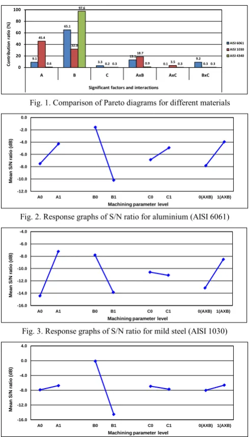
significant effect on surface roughness with a contribution ratio (P ≅ 65%), followed by cutting speed (A) (P ≅ 9%), and depth of cut (C) (P ≅ 3%). The interactions between cutting speed and feed rate (A×B) and feed rate and depth of cut (B×C) also played roles with contributing ratios (P ≅ 13%) and (P ≅ 9%) respectively. It is worth pointing out that the total contribution of the main effects is about 77% compared to the total contribution of the interaction effects of 23%. Therefore, it will be moderately difficult to optimise the diameter error by selection of input parameters.
The Pareto ANOVA analysis for mild steel (AISI 1030) is given in Table 5. It illustrates that cutting speed (A) has the most significant effect on surface roughness with a contribution ratio (P ≅ 45%), followed by feed rate (B) (P ≅ 31%), and depth of cut (C) (P ≅ 0.2%). The interactions between cutting speed and feed rate (A×B) and cutting and depth of cut (A×C) also played roles with contributing ratios (P ≅ 18%) and (P ≅ 3%) respectively. It is worth noting that the total contribution of the main effects remains roughly the same (about 78%), although in this case the contribution of cutting speed (A) is increased notably with expense of feed rate. As the total contribution of the interaction effects remains high (22%), it will be moderately difficult to optimise surface roughness by selection of input parameters.
The Pareto ANOVA analysis for alloy steel (AISI 4340) is given in Table 6. It shows that feed rate (B) has the most significant effect on surface roughness with a contribution ratio (P ≅ 98%). All other effects, both main and interaction effects, were almost negligible. Therefore, it will be relatively easy to optimise the surface roughness by selection of proper feed rate.
A comparison of Pareto diagrams for different materials is illustrated in Fig. 1, in which the dominant effect of feed rate on surface finish is evident. The effect of feed rate on surface roughness is well known, and most of the widely applied geometric models for surface roughness include feed rate and tool nose radius. However, results showed considerable interaction effects between cutting speed and feed rate, which influenced the surface finish. It appears that with the increase of material hardness the interaction effect diminishes.
Within the selected range of variation, depth of cut showed negligible effect on surface roughness (Fig. 1). Similar results have been reported by previous studies [9, 14-15]. The Pareto ANOVA analyses (Tables 4-6) showed that in all cases high cutting speed (A1) and low feed rate (B0) produced the best surface roughness, which is in line with conventional machining wisdom. The cutting speed must be selected high enough to avoid formation of a built up edge (BUE).
B. Response Tables and Graphs
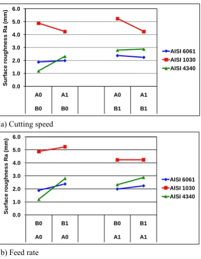
The response table and response graph for aluminium are illustrated in Table 7 and Fig. 2 respectively. As the slopes of the response graphs represent the strength of contribution, the response graphs confirm the findings of the Pareto ANOVA analysis given in Table 4. Fig. 2 shows that high level of depth of (C1) was the best depth of cut. Because the interaction A×B was significant, an A×B two-way table was applied to select their levels. The two-way table is not included in this paper due to space constraints. From the
A×B two-way table, the optimum combination of factors A and B in order to achieve a lowest surface finish was determined as A1B0. Therefore, the best combination of input variables for minimising surface roughness was A1B0C1; i.e., high level of cutting speed, low level of feed rate, and high level of depth of cut.
The response table and response graph for mild steel are illustrated in Table 8 and Fig. 3 respectively. The response graph confirms the findings of the Pareto ANOVA analysis given in Table 5. Low level of depth of (C0) was the best depth of cut (Fig. 3). From the A×B two-way table, the optimum combination of factors A and B in order to achieve a lowest surface finish was determined as A1B0.Therefore, the best combination of input variables for minimising surface roughness was A1B0C0; i.e., high level of cutting speed, low level of feed rate, and low level of depth of cut.
The response table and response graph for alloy steel are shown in Table 9 and Fig. 4 respectively. The response graph confirms the findings of the Pareto ANOVA analysis given in Table 6. Low level of depth of (C0) was the best depth of cut (Fig. 4). From the A×B two-way table the optimum combination of factors A and B was set to A1B0. Therefore, the best combination of input variables for minimising surface roughness was A1B0C0; high level of cutting speed, low level of feed rate, and low level of depth of cut.
C. Traditional Analysis
Variations in surface roughness for input parameters cutting speed and feed rate are illustrated in Fig. 5. Effect of depth of cut is omitted because it demonstrated negligible percent contribution in Pareto ANOVA analyses (Tables 4-6).
The graph shows that for aluminium and mild steel, with the increase of cutting speed surface roughness more or less remained steady or even deteriorated, whereas for alloy steel it improved considerably (Fig. 5a). The graph also shows that with the increase of feed rate the surface roughness values also increase, although this increase is higher at low cutting speed (Fig. 5b).
Fig. 5 demonstrates that, contrary to traditional machining wisdom, the material with the higher machinability rating did not always produce a better surface finish. Therefore, surface roughness by itself is not a reliable indicator of machinability. The reason behind this is that the optimum cutting conditions for different materials are different; whereas in our experiment we selected the same cutting parameters for all the materials selected, conservatively based on the optimum cutting condition suitable for the material most difficult to machine, alloy steel AISI 4340, primarily to protect the tool. Furthermore, due to the interaction effects between cutting speed and feed rate, surface roughness is not always related to machinability rating.
D. Regression Analysis
To establish the prediction model, the software package
XLSTAT was applied to perform the regression analysis
indicates that the prediction model has a satisfactory ‘goodness of fit’.
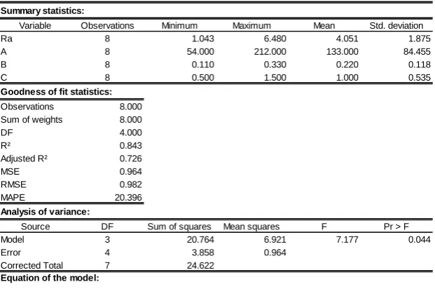
The regression analysis results and prediction model for mild steel are given in Table 11. In this case, the coefficient of determination (R2) is 0.843, which is slightly better compared to aluminium.
The regression analysis results and prediction model for alloy steel are given in Table 12. In this case, the coefficient of determination (R2) is 0.993, which shows the best ‘goodness of fit’ for the three materials selected. It is worth noting that ‘goodness of fit’ improved with material hardness (see hardness data given in Table 2) due to reduction of interaction effects.
Tables 10-12 show that the model equation for each material is different. It is worth pointing out that currently available geometric models do not work in practice because they do not consider the formation of BUE and change of tool profile caused by tool wear. Therefore, any future analytical model should include material characteristics to make it meaningful.
V. CONCLUDING REMARKS
From the experimental work conducted and the subsequent analysis, the following conclusions can be drawn:
Feed rate has a dominant effect on surface finish; the interaction between cutting speed and feed rate also plays a major role which is influenced by the properties of work material. With the increase of material hardness the interaction effect diminishes.
Within the selected range, depth of cut showed negligible effect on surface roughness.
Surface roughness by itself is not a reliable indicator of machinability, due to non-optimal cutting conditions and interaction effects of additional factors.
The model equations resulting from regression analysis for different materials show significant differences. Therefore, any future analytical model should include material aspect to make it meaningful.
ACKNOWLEDGMENT
The authors would like to acknowledge the contribution of Mr. Mohamad F. Jasni, a final year student at the Department of Mechanical Engineering, Curtin University (currently with Bondstrong Pty. Ltd., Success, Western Australia).
REFERENCES
[1] Droozda, T. J. and Wick, C. (Eds), Tool and Manufacturing Engineers Handbook, Vol. 1, Machining, SME, Dearborn, pp. 1-52.
[2] Sreejith, P. S., and Ngoi, B. R. A., “Dry Machining: Machining of the future”, J. of MaterialsProcessing Technology, Vol. 101, pp.
287-291, 2000.
[3] Davim, J.P., “A Note on the Determination of Optimal Cutting Conditions for Surface Finish Obtained in Turning Using Design of Experiments”, J. of Materials Processing Technology, Vol. 116, pp.
305-308, 2001.
[4] Manna, A., and Bhattacharyya, B., “A Study on Different Tooling System during Machining of Al/SiC-MMC”, J. of Materials Processing Technology, Vol. 123, pp. 476-481, 2002.
[5] Dilbag, S., and Rao, P.V., “A Surface Roughness Prediction Model for Hard Turning Process”, Int. J. of Advanced Manufacturing Technology, Vol. 32, pp. 1115-1124, 2006.
[6] Thamizhmanil, S., Saparudin, S., and Hasan, S., “Analysis of Surface Roughness by Turning Process using Taguchi Method”, J. of Achievements in Materials and Manufacturing Engineering, Vol. 20, pp. 503-506, 2007.
[7] Isik, Y., “Investigating the Machinability of Tool Steels in Turning Operations”, Materials & Design, Vol. 28, pp. 1417-1424, 2007
[8] Lalwani D.I., Mehta N.K., and Jain P.K., “Experimental Investigations of Cutting Parameters Influence on Cutting Forces and Surface Roughness in Finish Hard Turning of MDN250 Steel”, J. of MaterialsProcessing Technology, Vol. 206, pp. 167-179, 2008.
[9] Rafi, N. H. and Islam, M. N., “An Investigation into Dimensional Accuracy and Surface Finish Achievable in Dry Turning”, Machining Science and Technology, v. 13(4), pp. 571-589, 2009.
[10] Australian Standard, AS2536 Surface Texture, Standards Association
of Australia, 1982.
[11] Park, S.H., Robust Design and Analysis for Quality Engineering,
Chapman & Hall, London, 1996.
[12] Ross, P.J., Taguchi Techniques for Quality Engineering,
McGraw-Hill, New York, 1988.
[13] MatWeb, Material Property Data, Accessed through Internet
(19/2/2011),
[14] Dhar, N. R., Kamruzzaman, M. and Ahmed, M., “Effect of Minimum Quantity Lubrication (MQL) on Too Wear and Surface Roughness in Turning AISI-4340 Steel”, J.of Materials Processing Technology,
Vol. 172, pp. 299-304, 2006.
[15] Lima, J. G., Avila, R. F., Abrao, A. M., Faustino, M. & Davim, J. P., Hard Turning: AISI 4340 high strength low alloy steel and AISI D2 cold work tool steel. J. of Materials Processing Technology, Vol.
169, 388-395, 2005.
9.1 65.1
3.3 13.1
0.1 9.2 45.4
32.0 0.2
18.7
3.5 0.3 0.6
97.6
0.3 0.9 0.3 0.3 0
20 40 60 80 100
A B C AxB AxC BxC
Significant factors and interactions
Co
nt
ri
but
io
n
ra
tio
(
%
)
[image:4.595.304.549.330.759.2]AISI 6061 AISI 1030 AISI 4340
Fig. 1. Comparison of Pareto diagrams for different materials
-12.0 -10.0 -8.0 -6.0 -4.0 -2.0 0.0
A0 A1 B0 B1 C0 C1 0(AXB) 1(AXB)
M
ean
S
/N
rat
io
(
d
B)
Machining parameter level
Fig. 2. Response graphs of S/N ratio for aluminium (AISI 6061)
-16.0 -14.0 -12.0 -10.0 -8.0 -6.0 -4.0
A0 A1 B0 B1 C0 C1 0(AXB) 1(AXB)
M
ean
S
/N
rat
io
(
d
B)
Machining parameter level
Fig. 3. Response graphs of S/N ratio for mild steel (AISI 1030)
-16.0 -12.0 -8.0 -4.0 0.0 4.0
A0 A1 B0 B1 C0 C1 0(AXB) 1(AXB)
M
ean
S
/N
rat
io
(
d
B)
Machining parameter level
0.0 1.0 2.0 3.0 4.0 5.0 6.0
A0 A1 A0 A1
B0 B0 B1 B1
S
u
rf
ace
ro
u
g
h
n
ess R
a (
m
m
)
AISI 6061 AISI 1030 AISI 4340
(a) Cutting speed
0.0 1.0 2.0 3.0 4.0 5.0 6.0
B0 B1 B0 B1
A0 A0 A1 A1
S
u
rf
ace
ro
u
g
h
n
ess R
a (
m
m
)
AISI 6061 AISI 1030 AISI 4340
[image:5.595.69.271.47.307.2](b) Feed rate
Fig. 5. Variation of surface roughness for input patameters
Table 7. Respoonse table for mean S/N ratio for alumimium (AISI 6061)
Mean S/N ratio
Cutting parametrs Symbol Level 0 Level 1 Max -Min
[image:5.595.306.548.71.129.2]Cutting speed A -7.895 -6.764 1.131 Feed rate B -0.128 -14.530 14.402 Deapth of cut C -6.934 -7.724 0.790 Interaction AXB AXB -8.037 -6.622 1.416
Table 8. Respoonse table for mean S/N ratio for mild steel (AISI 1030)
Mean S/N ratio
Cutting parametrs Symbol Level 0 Level 1 Max -Min
[image:5.595.306.548.163.222.2]Cutting speed A -7.515 -4.304 3.211 Feed rate B -1.617 -10.201 8.584 Deapth of cut C -6.878 -4.940 1.937 Interaction AXB AXB -7.838 -3.981 3.857
Table 9. Respoonse table for mean S/N ratio for alloy steel (AISI 4340)
Mean S/N ratio
Cutting parametrs Symbol Level 0 Level 1 Max -Min
[image:5.595.304.548.254.314.2]Cutting speed A -14.460 -7.243 7.217 Feed rate B -7.823 -13.881 6.058 Deapth of cut C -10.605 -11.099 0.494 Interaction AXB AXB -13.169 -8.534 4.635
Table 4. Pareto ANOVA analysis for aluminium (AISI 6061) Factor and interaction
A B AxB C AxC BxC
0 -7.51 -1.62 -7.84 -6.88 -5.76 -7.52
1 -4.30 -10.20 -3.98 -4.94 -6.05 -4.29
Sum of squares of difference (S) 10.31 73.69 14.88 3.75 0.08 10.43
Contribution ratio (%) 9.11 65.13 13.15 3.32 0.07 9.22
Pareto diagram
Cumulative contribution 65.13 78.28 87.50 96.61 99.93 100.00
Check on significant interaction
Optimum combination of significant factor levelA1B0C1
Sum at factor level
AxB two-way table
AxC
Table 5. Pareto ANOVA analysis for mild steel (AISI 1030) Factor and interaction
A B AxB C AxC BxC
0 -57.84 -31.29 -52.68 -42.42 -47.39 -42.21
1 -28.97 -55.52 -34.14 -44.39 -39.43 -44.60
Sum of squares of difference (S) 833.31 587.22 343.75 3.90 63.40 5.71
Contribution ratio (%) 45.36 31.96 18.71 0.21 3.45 0.31
Pareto diagram
Cumulative contribution 45.36 77.32 96.03 99.48 99.79 100.00
Check on significant interaction
Optimum combination of significant factor levelA1B0C0
Sum at factor level
AxB two-way table
C
Table 6. Pareto ANOVA analysis for alloy steel (AISI 4340) Factor and interaction
A B AxB C AxC BxC
0 -7.89 -0.13 -8.04 -6.93 -6.94 -6.94
1 -6.76 -14.53 -6.62 -7.72 -7.72 -7.71
Sum of squares of difference (S) 1.28 207.42 2.00 0.62 0.61 0.59
Contribution ratio (%) 0.60 97.60 0.94 0.29 0.29 0.28
Pareto diagram
Cumulative contribution 97.60 98.54 99.14 99.44 99.72 100.00
Check on significant interaction
Optimum combination of significant factor levelA1B0C0 AxB two-way table
Sum at factor level
BxC
[image:5.595.156.438.332.781.2]Table 10. Results of regression analysis for aluminium (AISI 6061)
Summary statistics:
Variable Observations Minimum Maximum Mean Std. deviation
Ra 8 0.590 3.533 2.305 1.146
A 8 54.000 212.000 133.000 84.455
B 8 0.110 0.330 0.220 0.118
C 8 0.500 1.500 1.000 0.535
Goodness of fit statistics:
Observations 8.000
Sum of weights 8.000
DF 4.000
R² 0.815
Adjusted R² 0.677
MSE 0.424
RMSE 0.651
MAPE 22.951
Analysis of variance:
Source DF Sum of squares Mean squares F Pr > F
Model 3 7.490 2.497 5.887 0.060
Error 4 1.696 0.424
Corrected Total 7 9.187
Equation of the model:
[image:6.595.142.453.314.520.2]Ra = 0.913 - 2.579*10-3*A + 8.572*B - 0.151*C
Table 11. Results of regression analysis for mild steel (AISI 1030)
Summary statistics:
Variable Observations Minimum Maximum Mean Std. deviation
Ra 8 1.043 6.480 4.051 1.875
A 8 54.000 212.000 133.000 84.455
B 8 0.110 0.330 0.220 0.118
C 8 0.500 1.500 1.000 0.535
Goodness of fit statistics:
Observations 8.000
Sum of weights 8.000
DF 4.000
R² 0.843
Adjusted R² 0.726
MSE 0.964
RMSE 0.982
MAPE 20.396
Analysis of variance:
Source DF Sum of squares Mean squares F Pr > F
Model 3 20.764 6.921 7.177 0.044
Error 4 3.858 0.964
Corrected Total 7 24.622
Equation of the model:
Ra = 4.363 - 1.615*10-2*A + 8.924*B - 0.128*C
Table 12. Results of regression analysis for alloy steel (AISI 4340)
Summary statistics:
Variable Observations Minimum Maximum Mean Std. deviation
Ra 8 0.860 5.527 3.183 2.303
A 8 54.000 212.000 133.000 84.455
B 8 0.110 0.330 0.220 0.118
C 8 0.500 1.500 1.000 0.535
Goodness of fit statistics:
Observations 8.000
Sum of weights 8.000
DF 4.000
R² 0.993
Adjusted R² 0.988
MSE 0.062
RMSE 0.250
MAPE 8.198
Analysis of variance:
Source DF Sum of squares Mean squares F Pr > F
Model 3 36.875 12.292 197.161 < 0.0001
Error 4 0.249 0.062
Corrected Total 7 37.124
Equation of the model:
[image:6.595.141.453.568.768.2]![Table 1. Properties of work materials [13]](https://thumb-us.123doks.com/thumbv2/123dok_us/1289377.657978/2.595.306.548.317.377/table-properties-of-work-materials.webp)