Abstract—Efficient communication is still a severe problem
in many parallel codes. Therefore, we will discuss the advantages of bitonic sorting networks for the organisation of data exchange among nodes in a parallel program. Via data flow analysis we will find fixpoints of bitonic sorting networks and see how to exploit those for obtaining correction methods that allow to solve the packet problem with (log N) steps.
Index Terms—bitonic sorting networks, data flow analysis,
fixpoints, efficient communication, structure mechanics
I. INTRODUCTION
NE major problem in parallel computing is to find efficient communication strategies. Frequent data transmissions easily lead to a tremendous communication advent that dominates the computation and, thus, spoils any speed-up and scalability values. Especially when considering several hundred thousand cores, scalability plays a significant role on the step to ‘exascale’ computing.
Whenever data should be exchanged in parallel between
all nodes (we use the term node substitutional for process, core, processor or computer) of a parallel program, the main question is concerning the total amount of necessary communication steps to be carried out. For a more generic approach (following the example of Valiant [1]) we assume to have N nodes labelled from 0 to N1 where each node
stores one packet to be sent to another node. In case all packet destinations are distinct the communication pattern follows a permutation. In [1], Valliant has proposed a
(log N) algorithm for N = 2n nodes which is executed on
an n-dimensional binary cube. The main idea of his
algorithm is to separate communication into two phases, where in the first phase each node sends its packet to a randomly chosen node and in the second phase packets are further transmitted to a node randomly chosen of a set of nodes, thus, the distance to the packet’s destination becomes shorter.
One strong point of this algorithm is to achieve the communication in (log N) steps for every permutation, i.e.
independent of the initial packet destinations as well as for partial permutations. Nevertheless, there are also some weak points which make the practical usage especially for nowadays supercomputers difficult. First of all, nodes are assumed to have queues in order to store more than one
Manuscript received July 26, 2011; revised August 16, 2011.
Computation in Engineering, Technische Universität München, Arcisstrasse 21, 80290 München, GERMANY. Corresponding author contact: phone: +49-89-289-25057; fax: +49-89-289-25051; e-mail: [email protected]
packet at a time. Hence, there is a (strong) sequential part in the communication as not all packets might be in transmission at the same time. Second, Valiant assumes an
n-dimensional binary cube where each node has n wires
from it—such a topology is rarely found among the world’s fastest supercomputers.
Other approaches such as bitonic sorting networks proposed by Batcher [2] yield with (log2
N) necessary
steps an inferior performance on the one hand, but they are much simpler to implement as efficient communication pattern on arbitrary network topologies on the other hand; see [3] for a sample application. There are many more strategies concerning topologies, protocols, and communication patterns in order to further reduce the complexity (see [4] e.g.), but at this point we would like to focus on bitonic sorting networks (BSN) as they fulfill certain aspects such as synchronous transmission (i.e. the absence of waiting queues) and determinism (i.e. no random choice of nodes). According to Valiant, another weak point of BSNs is the missing capability to do partial permutations, but this is of no importance for our purposes.
Instead, we will address a different set of problems related to fixpoints of BSNs and their consequences on
efficient communication strategies for the aforementioned permutations of packets among all nodes. Hence, the reminder of this paper is as follows. In chapter 2, we will introduce a data flow analysis of BSNs to reveal fixpoints of those networks, while in chapter 3 we will propose a solution to this problem and highlight the use of this communication strategy to a sample application from structure mechanics. Finally, we will close in chapter 4 with a short summary and an outlook.
II. DATA FLOW ANALYSIS OF BITONIC SORTING NETWORKS
A. Bitonic Sorting Networks
Bitonic sorting networks were introduced by Batcher [2] as an alternative to ‘classical’ sorting algorithms that can do the sorting in parallel with a complexity of (log2
N) in case
of N 2n input data for some integer n (see [5], e.g., for
BSNs of arbitrary sizes N). Therefore, the BSN is organised
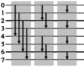
in two phases. In the first phase, any arbitrary input sequence is modified to become a bitonic sequence, before in the second phase this sequence is finally sorted by executing a bitonic merge. A bitonic merge (as depicted in Fig. 1 for eight inputs) needs (log N) steps to sort any
bitonic sequence in ascending or descending order. Creating a bitonic sequence out of any arbitrary sequence takes
(log2
N) steps, hence the total cost of a BSN can be
Efficient Bitonic Communication for the
Parallel Data Exchange
Ralf-Peter Mundani, Ernst Rank
computed as (log2
N). Omitting phase one might lead to
wrong results as further discussed in the next section.
Applying the bitonic merge scheme as communication pattern to parallel applications, an efficient data transfer between the nodes of a parallel program is possible. For instance, a total exchange among all nodes could be easily implemented carrying out all data transmissions in parallel. As at no point in time one node has to store more than one data item, no queues are necessary and, thus, all transmissions can be done synchronously. Assuming a high enough bisection bandwidth of the underlying physical network topology, a bitonic merge communication pattern can benefit and exploit the network performance in order to reduce the overall communication time.
For Valiant’s example this means, that every node stores one packet labelled by a destination address of any of the other nodes. As long as all addresses are distinct, the bitonic merge can handle the transfer of all packets in (log N)
steps—unfortunately not for all possible permutations. There exists a subset PП of all possible permutations П
for which the transfer leads to an incorrect result, i.e. some packets were delivered to a wrong address. Hence the question arises for which permutations pП this happens
and what can be done as ‘correction method’ in order to leverage the simple implementation of a bitonic merge communication pattern for the efficient data transfer in parallel programs.
B. Data Flow Analysis
To reveal all permutations that lead to incorrect results a closer look has to be paid on the structure of BSNs. Here, the single data movement between two nodes (in one stage of the bitonic merge) is of primary interest which suggests the idea of performing a data flow analysis of a BSN. Data flow analysis is a proper way whenever it comes to the understanding and optimisation of algorithms. In our case, a closer look on the data flow inside a BSN will help to identify the problematic permutations. Therefore, we have to trace the single packets on their way through the bitonic merge in order to observe when something goes wrong and an incorrect state (for the rest of this paper we refer to the output or result of a bitonic merger as state) is achieved.
As a bitonic merge with N inputs has a total of N!
permutations, hence for large values of N a data flow
analysis is no longer feasible. According to [6] the problem can be simplified by considering 0-1-bit vectors instead of arbitrary input data as any network sorts correct any input
data if and only if it also sorts all possible 0-1-bit vectors. This ‘reduces’ the complexity from N! to 2N, nevertheless
still not very practicable for large values of N. Again, N
determines the amount of nodes in our parallel program and for modern supercomputers N tends to be larger than 105 or
106 easily.
Let’s consider a sample scenario. As input we have the 0-1-bit vector (0100 0100)T that is processed by the bitonic merger in the following way. The two 1’s arrive at input #1 and #5 at the same time where they clash, i.e. the comparator keeps one 1 in the upper half and one in the lower half of the bitonic merger. Further processing then leads to the following state (0001 0001)T. As this bit vector is not sorted (i.e. (0000 00011)T) it is wrong and, thus, would not be a correct solution to our packet problem. The same result can be observed for bit vectors (1000 1000)T, (0010 0010)T, and (0001 0001)T.
In order not to follow up all 28 possible bit vectors for this case, a more general analysis would be preferable. As we can see from the above example, four different inputs lead to the same wrong state. Hence, the question should not be how many inputs lead to wrong states, but how many wrong states do exist as they play a special role in our further considerations. For our example with N 8 there are
11 of those incorrect states shown as follows according to their amount of 1’s.
2: (0001 0001)T, (0000 0101)T
3: (0001 0101)T, (0001 0011)T
4: (0101 0101)T, (0011 0011)T, (0001 0111)T
5: (0101 0111)T, (0011 0111)T
6: (0101 1111)T, (0111 0111)T
What can be observed immediately is that there are never more 1’s in the upper half (or first part) than in the lower half (or second part) as at most K/2 1’s can clash in the
same step (and thus stay up) in case of K 1’s. As this
follows a recursive pattern – a bitonic merger of 2n1 inputs contains all states of a bitonic merger with 2n inputs – all of
those wrong states can be built from combinations of the 1-distributions in subsequent halves. For instance, in case of three 1’s in the input data only one 1 might clash and reside in the upper half, i.e. (0001 )T. For the lower half only the combinations ( 0101)T and ( 0011)T are feasible – both combinations of a bitonic merger with four inputs – as due to the structure of the bitonic merger all 1’s are always shifted downward as far as possible. Hence, in case all three 1’s reside in the lower half, only the vector (0000 0111)T is possible but this does not correspond to an incorrect state.
As it’s clear how to construct the incorrect states of a bitonic merger with N 2n inputs, the total amount of those
states as well as the states itself are computable. This is an important property for the next section in order to further evaluate BSNs for the handling of the packet problem in case of arbitrary, i.e. not only bitonic, sequences in (log N)
[image:2.595.100.236.88.195.2]steps. Fig. 1. Bitonic merge of N 8 inputs with (log N) 3 steps (grey boxes)
C. Fixpoints
If a permutation p leads to an incorrect state s, one idea
might be to process this state again as input to the same bitonic merger. Unfortunately it turns out, that the incorrect states are fixpoints of the bitonic merger bm( ) as the
mapping bm(s) s is true for all sSП with S denoting
the subset of incorrect states. We have seen in the section above that several different permutations pP, with P
denoting the subset of all permutations leading to an incorrect state, might lead to the same incorrect state s,
namely the one where all 1’s are shifted downward as far as possible. Hence, only those states have to be further considered as otherwise there exists a mapping bm(p) s.
Proof 1: sS: bm(s) s is true
If s is an incorrect state then the corresponding bit vector
must have at least one 0-bit bi, 0 lim 2n, between
two 1-bits bl and bm—otherwise it would consist of some 0’s
followed only by 1’s indicating a correct sorting. In each step of the bitonic merge some upper part is compared to some lower part and corresponding bits are exchanged if being out of order. Hence, if bi is in the upper part and
compared to a 1 in the lower part bi doesn’t change its place
and the final result is the same as the input sequence, i.e.
bm(s) s. If bi is in the lower part and compared to a 1 in
the upper part they are exchanged and, thus, the bits between bl and bm are filled with 1’s. But this leads to a
correct sorting which contradicts the assumption that sS
was an incorrect state □
Proof 2: pPpS: sS with bm(p) s
Due to the assumption pP the bit vector contains at
least two bits bi and bj with 0 ij 2n and bibj 1 that
clash in the kth step with 1 kn. Hence, there is at least
one 0 between the two 1’s such that the final bit vector has a structure as follows (101)T and corresponds to a critical state—otherwise, i.e. kn, bits bi and bj would be
[image:3.595.360.495.461.566.2]neighbours without any 0 in between. But this leads to a correct state, so the input sequence must have been bitonic and, thus, contradicts the assumption pP. According to
Fig.°1 all 1’s of the bit vector are shifted downward as long as they do not clash. Hence, if no shifting can be done
pbm(p) such that p belongs to S, but this is a
contradiction to the assumption pS. Therefore, pbm(p)
which means at least one shifting was executed. Now feeding the resulting bit vector bm(p) again as input to the
bitonic merger the shifting can be continued until we reach a critical state sS, such that there exists a mapping bm(p) s □
Knowing that all incorrect states are fixpoints of a bitonic merger and all problematic input sequences lead to such fixpoints, this allows us restricting further investigations on those fixpoints only. Again, the total amount of incorrect states (of a bitonic merger with a certain size N 2n) is an
important characteristic telling us how many ‘special cases’ we have to consider for any correction method in order to
prove that the bitonic merger leads for all permutations to the correct results. In case of N 4, N 8, N 16, or N 32
inputs the total amount of incorrect states is still quite moderate with only 1, 11, 151, or 7548 states, resp, and thus can be easily checked by an algorithm. In the next chapter we will therefore discuss about possible correction methods as well as a sample application from structure mechanics.
III. APPLICATION OF BSNCOMMUNICATION STRATEGY For further considerations we assume that in case between two nodes a clash occurs, both of the nodes set a local flag notifying that the bitonic merge leads to an incorrect state. When finished, all nodes exchange flags in order to indicate that more processing, i.e. an additional correction is necessary.
A. Naïve Correction: Odd-Even-Transposition
One idea to handle incorrect states is firstly to ‘crack’ a fixpoint s (applying some shifts e.g.) and then process this
modified state s again by the bitonic merger. In the ideal
case, now bm(s) leads to a correct result—otherwise bm(s) s with sS, i.e. another fixpoint has been
reached and the entire correction has to be repeated until the problem is solved. Immediately two questions arise: How to crack a fixpoint and how many rounds of bitonic merge have to be executed until a correct result is achieved?
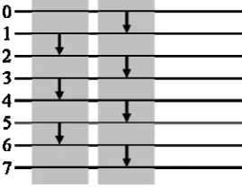
A naïve approach for cracking a fixpoint is to deploy some phases of an even-transposition. During an odd-even-transposition neighbouring nodes either starting with odd or even indices are pairwise compared and exchanged if being out of order. Fig. 2 shows the related comparisons in case of N 8 inputs.
If we now consider the 11 incorrect states (as illustrated above) of a BSN with N 8 inputs it is simple to check if
this correction method works by applying the odd-even-transposition on each of them. For seven states the problem can be solved while for four states the odd-even-transposition leads to another fixpoint. Hence, for the latter states a further processing via another round through the bitonic merger is ineffective. The resulting incorrect states are shown as follows according to their amount of 1’s.
2: (0000 0101)T
4: (0001 0111)T
6: (0101 1111)T
Fig. 2. Two phases (grey boxes) of an odd-even-transposition for N 8
A slight better result can be achieved if only the first of the two phases of an odd-even-transposition (namely the first grey box in Fig. 2) is performed, followed by a complete round of the bitonic merger. Considering the same 11 incorrect states from above, this is – again – trivial to check. Now for nine states the problem can be solved while only two states lead to another fixpoint where further processing via the bitonic merger is ineffective. The resulting incorrect state (according to its amount of 1’s) is as follows.
4: (0001 0111)T
One interesting observation is that all incorrect states with an odd number of 1’s could be solved and, thus, only states with an even number of 1’s are left. But at this point we do not claim that this is a general principle which all fixpoints of any BSN with size 2n follow; something that could be
further investigated in the future. Deploying a second round of an odd-even-transposition finally solves the problem for the three incorrect states or the one incorrect state above in case of two phases or one phase of an odd-even-transposition, resp., as correction method. Hence, this leads to our second question of how many times the correction method has to be applied on a BSN of arbitrary size until any 0-1-bit vector is sorted.
Proof 3: For any BSN with size N 2n the correction
method has to be deployed at most log N times.
For any fixpoint s the corresponding bit vector must have
at least one 0-bit bi, 0 lim 2n, between two 1-bits bl
and bm. Due to the odd-even-transposition the 1-bit bl is
shifted downward by one position (it can be seen easily that
l has to be an even index, otherwise s would not be a
fixpoint and a mapping bm(s) s with sS would exist).
Either the ‘gap’ between bl and bm has been closed and a
correct state has been reached, or the bit vector is processed again by the BSN otherwise. In the latter case, if bl has
clashed before the odd-even-transposition in step k, now it
might clash in a step k1 or lead to a correct result. Hence,
as the bitonic merger consists in total of log N steps, and
each odd-even-transposition postpones the clashing at least by one step, there can be at most log N full processing
rounds □
B. Further Considerations on Complexity
Up to now we have seen that for the packet problem proposed by Valiant a BSN can solve the task with log N
steps, but unfortunately not for all permutations of input data. Some permutations might lead to incorrect states that are furthermore fixpoints of the BSN. Hence, for any correction method it is enough to consider only those very limited amount of fixpoints which makes any checking much simpler. Nevertheless, what’s left to show is that the bitonic merge plus any correction method is still in the range of (log N) or at least clog N with some constant
factor c log N.
Instead of a formal prove (which at this point is also very difficult to show) we choose an algorithmic approach. What
can be observed for BSN of size N 2n with increasing n is
that the majority of all permutations ( 90%) lead to an incorrect state. Fortunately, there are much less fixpoints that have to be further considered. Hence, for any correction method applied to those fixpoints it can be shown by an algorithm how many correction steps it takes until the fixpoints have been fully resolved.
Concerning now exascale computing this becomes interesting for values of N 220 which entails some
computational effort to prove for all critical states. Nevertheless, for smaller values of N we could show that
the majority of all fixpoints was resolved after just one correction step (1-fixpoints) and only very few fixpoints needed further processing, i.e. more than one correction step (2-fixpoints, 3-fixpoints and so on). We furthermore could observe a trend that for increasing values of N the ratio of
1-fixpoints stays pretty stable, hence we assume this also holds for larger values of N—something that has to be
further investigated in the future.
Based on this very promising results we conclude so far: the majority of fixpoints are 1-fixpoints and higher representatives (2-, 3-, …-fixpoints) have a strictly decreasing ratio, thus, in most cases c 1 is enough. If we
now consider the average case, it takes only a few correction steps c log N in order to reach a correct state.
For the initially proposed packet problem this means that the bitonic merge can solve any permutation on average with
(log N) steps.
C. Sample Application: FEM
One application that benefits from the BSN communication strategy is related to structure mechanics. Here, with the p-version of finite element methods (p-FEM)
– without going into detail of high-order FEM, see [7] or [8] for further information – arises the problem to assemble the global system matrix K from the single element stiffness
matrices K(e) via superposition KK(e). As K might grow
very large, usually memory is the limiting factor. Nevertheless, p-FEM is very well suited for parallelisation
as the single element stiffness matrices K(e) are independent
from each other and, thus, can be computed in parallel. When it comes to the matrix assembly of K, efficient
parallel strategies can be found in literature for shared memory systems (see [9] e.g.) while distributed memory approaches typically suffer from a huge communication advent. The problem is that within a distributed assembly each process computes only one block of K for which it
needs certain K(e)’s as input data. Even the computation of
single K(e)’s can be optimised concerning locality measures,
i.e. they are computed on the same node where they are needed for the assembly, most of them are needed on several nodes and, thus, have to be transmitted. In accordance to the packet problem from above one K(e) can
be seen as a packet that has to be sent from one node to some destination.
In a worst case approach – which of course never meets reality – each node stores some K(e)’s or packets, resp.,
steps. As each node is source (and destination) of M
packets, we assume that each node has the capacity to store
M packets for later delivery. In contrast to the single packet
problem each node will first of all do M transmissions in a
row (transmissions among all disjoint pairs of nodes still happen in parallel while several transmissions between two nodes happen sequentially) before the nodes decide which packets to keep for local processing, i.e. a packet has arrived at its final destination, and which for further transfer.
Practically the M-packet problem can be seen as a
sequence of M rounds of the single packet problem. For the
single packet problem we have seen that any incorrect state can be corrected using one of the methods shown above. Hence, this is also valid in case of M packets with a small
modification. In order to distinguish the packets they have to be labelled from 1 to M where the ordering of the packets
under no circumstance must be subject to change. Otherwise it is not possible to guarantee that any incorrect state might be resolved. Furthermore, each node needs M flags to
indicate any clash of packets during round m with m [1, M]. When finished with all transmissions there are
at most M incorrect states that can be treated in the usual
way. However, as this part is still work in progress, practical experiments have to show how many incorrect states appear on average for different values of M.
IV. CONCLUSIONS AND OUTLOOK
In this paper, we have presented an analysis of bitonic sorting networks as efficient communication strategy with a complexity of (log N) communication steps. BSNs have
proven to be a realistic alternative to existing approaches that in most cases require either special network topologies or sophisticated routing protocols while a BSN communication pattern is simple to implement even for arbitrary networks. We further have addressed the problem that a BSN only works correct for certain input sequences and, thus, might lead to incorrect states which have to be further processed. Those incorrect states are fixpoints of the BSN which can be computed in advance in order to find correction methods that do not exceed the (log N) property
and make the shown approach competitive.
For practical issues we have also given an example from structural mechanics that benefits from the BSN communication pattern when performing a distributed matrix assembly. Here, an efficient organisation of the data exchange among all nodes can tremendously reduce the communication advent and provide a scalable approach that is still advantageous on next generation supercomputers with more than 105 or 106 cores. Future work will comprise beside the search for further correction methods to the critical states especially an implementation of the distributed matrix assembly on a supercomputer in order to study the scalability and speed-up behaviour of the BSN communication pattern for different problem sizes and different amount of cores.
ACKNOWLEDGMENT
This publication is based on work supported by Award No. UK-C0020 made by King Abdullah University of
Science and Technology (KAUST). REFERENCES
[1] L. G. Valiant, “A scheme for fast parallel communication,” SIAM
Journal on Computing, vol. 11, no. 2, pp. 350361, 1982.
[2] K. E. Batcher, “Sorting networks and their applications,” in Proc. AFIPS Spring Joint Computer Conference, 1968, pp. 307314.
[3] J. F. Prins, “Efficient bitonic sorting of large arrays on the MasPar MP-1,” technical report TR91-041, Department of Computer Science,
UNC-Chapel Hill, USA, 1991.
[4] S. Rao, T. Suel, T. Tsantilas, M. Goudreau, “Efficient communication using total exchange,” in Proc. 9th International Parallel Processing Symposium, 1995, pp. 544550.
[5] T. Levi, A. Litman, “Bitonic sorters of minimal depth,” technical report CS-2010-08, Computer Science Department, Technion, Israel, 2010.
[6] D. E. Knuth, “The art of computer programming, vol. 3: Sorting and searching,” 2nd ed., Addison-Wesley, 1988.
[7] B. A. Szabó, I. Babuška, “Finite Element Analysis,” John Wiley & Sons, 1991.
[8] B. A. Szabó, A. Düster, E. Rank, “The p-version of the finite element method,” Encyclopedia of Computational Mechanics, vol. 1, chapter
5, pp. 119139, John Wiley & Sons, 2004.
[9] M. N. de Rezende, J. B. de Paiva, “A parallel algorithm for stiffness matrix assembly in a shared memory environment,” Computers and