Distributional Memory: A General Framework for Corpus Based Semantics

Framework for Corpus-Based Semantics

Marco Baroni

Alessandro Lenci

Research into corpus-based semantics has focused on the development of ad hoc models that treat single tasks, or sets of closely related tasks, as unrelated challenges to be tackled by extracting different kinds of distributional information from the corpus. As an alternative to this “one task, one model” approach, the Distributional Memory framework extracts distributional information once and for all from the corpus, in the form of a set of weighted word-link-word tuples arranged into a third-order tensor. Different matrices are then generated from the tensor, and their rows and columns constitute natural spaces to deal with different semantic problems. In this way, the same distributional information can be shared across tasks such as modeling word similarity judgments, discovering synonyms, concept categorization, predicting selectional preferences of verbs, solving analogy problems, classifying relations between word pairs, harvesting qualia structures with patterns or example pairs, predicting the typical properties of concepts, and classifying verbs into alternation classes. Extensive empirical testing in all these domains shows that a Distributional Memory implementation performs competitively against task-specific al-gorithms recently reported in the literature for the same tasks, and against our implementations of several state-of-the-art methods. The Distributional Memory approach is thus shown to be tenable despite the constraints imposed by its multi-purpose nature.

1. Introduction

The last two decades have seen a rising wave of interest among computational linguists and cognitive scientists in corpus-based models of semantic representation (Grefenstette 1994; Lund and Burgess 1996; Landauer and Dumais 1997; Sch ¨utze 1997; Sahlgren 2006; Bullinaria and Levy 2007; Griffiths, Steyvers, and Tenenbaum 2007; Pad ´o and Lapata 2007; Lenci 2008; Turney and Pantel 2010). These models, variously known as vector spaces, semantic spaces, word spaces, corpus-based semantic models, or, using the term we will adopt,distributional semantic models(DSMs), all rely on some version of the distributional hypothesis (Harris 1954; Miller and Charles 1991), stating that the degree of semantic similarity between two words (or other linguistic units) can be modeled

∗Center for Mind/Brain Sciences (CIMeC), University of Trento, C.so Bettini 31, 38068 Rovereto (TN), Italy. E-mail:[email protected].

∗∗Department of Linguistics T. Bolelli, University of Pisa, Via Santa Maria 36, 56126 Pisa (PI), Italy. E-mail:[email protected].

as a function of the degree of overlap among their linguistic contexts. Conversely, the format of distributional representations greatly varies depending on the specific aspects of meaning they are designed to model.

The most straightforward phenomenon tackled by DSMs is what Turney (2006b) calls attributional similarity, which encompasses standard taxonomic semantic rela-tions such as synonymy, co-hyponymy, and hypernymy. Words like dogand puppy, for example, are attributionally similar in the sense that their meanings share a large number of attributes: They are animals, they bark, and so on. Attributional similarity is typically addressed by DSMs based on word collocates (Grefenstette 1994; Lund and Burgess 1996; Sch ¨utze 1997; Bullinaria and Levy 2007; Pad ´o and Lapata 2007). These collocates are seen as proxies for various attributes of the concepts that the words denote. Words that share many collocates denote concepts that share many attributes. Bothdogandpuppymay occur nearowner,leash, andbark, because these words denote properties that are shared by dogs and puppies. The attributional similarity between dogandpuppy, as approximated by their contextual similarity, will be very high.

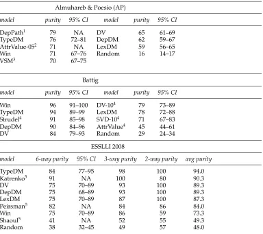
DSMs succeed in tasks like synonym detection (Landauer and Dumais 1997) or concept categorization (Almuhareb and Poesio 2004) because such tasks require a mea-sure of attributional similarity that favors concepts that share many properties, such as synonyms and co-hyponyms. However, many other tasks require detecting different kinds of semantic similarity. Turney (2006b) definesrelational similarityas the property shared by pairs of words (e.g, dog–animal and car–vehicle) linked by similar semantic relations (e.g., hypernymy), despite the fact that the words in one pair might not be attributionally similar to those in the other pair (e.g.,dogis not attributionally similar to car, nor isanimaltovehicle). Turney generalizes DSMs to tackle relational similarity and represents pairs of words in the space of the patterns that connect them in the corpus. Pairs of words that are connected by similar patterns probably hold similar relations, that is, they are relationally similar. For example, we can hypothesize that dog–tailis more similar tocar–wheelthan todog–animal, because the patterns connectingdogand tail(of,have, etc.) are more like those ofcar–wheelthan like those ofdog–animal(is a,such as, etc.). Turney uses the relational space to implement tasks such as solving analogies and harvesting instances of relations. Although they are not explicitly expressed in these terms, relation extraction algorithms (Hearst 1992, 1998; Girju, Badulescu, and Moldovan 2006; Pantel and Pennacchiotti 2006) also rely on relational similarity, and focus on learning one relation type at a time (e.g., finding parts).

a sort of “topical” relatedness between words: They might find, for example, a relation betweendogandfidelity. Topical relatedness, addressed by DSMs based on document distributions such as LSA (Landauer and Dumais 1997) and Topic Models (Griffiths, Steyvers, and Tenenbaum 2007), is not further discussed in this article.

DSMs have found wide applications in computational lexicography, especially for automatic thesaurus construction (Grefenstette 1994; Lin 1998a; Curran and Moens 2002; Kilgarriff et al. 2004; Rapp 2004). Corpus-based semantic models have also at-tracted the attention of lexical semanticists as a way to provide the notion of synonymy with a more robust empirical foundation (Geeraerts 2010; Heylen et al. 2008). Moreover, DSMs for attributional and relational similarity are widely used for the semi-automatic bootstrapping or extension of terminological repositories, computational lexicons (e.g., WordNet), and ontologies (Buitelaar, Cimiano, and Magnini 2005; Lenci 2010). Inno-vative applications of corpus-based semantics are also being explored in linguistics, for instance in the study of semantic change (Sagi, Kaufmann, and Clark 2009), lexical variation (Peirsman and Speelman 2009), and for the analysis of multiword expressions (Alishahi and Stevenson 2008).

The wealth and variety of semantic issues that DSMs are able to tackle confirms the importance of looking at distributional data to explore meaning, as well as the maturity of this research field. However, if we looked from a distance at the whole field of DSMs we would see that, besides the general assumption shared by all models that information about the context of a word is an important key in grasping its meaning, the elements of difference overcome the commonalities. For instance, DSMs geared towards attributional similarity represent words in the contexts of other (content) words, thereby looking very different from models that represent word pairs in terms of patterns linking them. In turn, both these models differ from those used to explore concept properties or argument alternations. The typical approach in the field has been a local one, in which each semantic task (or set of closely related tasks) is treated as a separate problem, that requires its own corpus-derived model and algorithm, both optimized to achieve the best performance in a given task, but lacking generality, since they resort to specific distributional representations, often complemented by additional task-specific resources. As a consequence, the landscape of DSMs looks more like a jigsaw puzzle in which different parts have been completed and the whole figure starts to emerge from the fragments, but it is not clear yet how to put everything together and compose a coherent picture.

network of semantic information that has been adapted to all sorts of tasks, many of them certainly not envisaged by the resource creators. We think that it is not by chance that no comparable resource has emerged from DSM development.

In this article, we want to show that a unified approach is not only a desirable goal, but it is also a feasible one. With this aim in mind, we introduceDistributional Memory(DM), a generalized framework for distributional semantics. Differently from other current proposals that share similar aims, we believe that the lack of generalization in corpus-based semantics stems from the choice of representing co-occurrence statistics directly as matrices—geometrical objects that model distributional data in terms of binary relations between target items (the matrix rows) and their contexts (the matrix columns). This results in the development of ad hoc models that lose sight of the fact that different semantic spaces actually rely on the same kind of underlying distributional information. DM instead represents corpus-extracted co-occurrences as a third-order tensor, a ternary geometrical object that models distributional data in terms of word– link–word tuples. Matrices are then generated from the tensor in order to perform se-mantic tasks in the spaces they define. Crucially, these on-demand matrices are derived from the same underlying resource (the tensor) and correspond to different “views” of the same data, extracted once and for all from a corpus. DM is tested here on what we believe to be the most varied array of semantic tasks ever addressed by a single distributional model. In all cases, we compare the performance of several DM imple-mentations to state-of-the-art results. While some of the ad hoc models that were devel-oped to tackle specific tasks do outperform our most successful DM implementation, the latter is never too far from the top, without any task-specific tuning. We think that the advantage of having a general model that does not need to be retrained for each new task outweighs the (often minor) performance advantage of the task-specific models.

The article is structured as follows. After framing our proposal within the general debate on co-occurrence modeling in distributional semantics (Section 2), we introduce the DM framework in Section 3 and compare it to other unified approaches in Section 4. Section 5 pertains to the specific implementations of the DM framework we will test experimentally. The experiments are reported in Section 6. Section 7 concludes by summarizing what we have achieved, and discussing the implications of these results for corpus-based distributional semantics.

2. Modeling Co-occurrence in Distributional Semantics

Corpus-based semantics aims at characterizing the meaning of linguistic expressions in terms of their distributional properties. The standard view models such properties in terms of two-way structures, that is, matrices coupling target elements (either single words or whatever other linguistic constructions we try to capture distributionally) and contexts. In fact, the formal definition of semantic space provided by Pad ´o and Lapata (2007) is built around the notion of a matrix M_|B|×|T|, withBthe set of basis elements representing the contexts used to compare the distributional similarity of the target elementsT.

in or close to the context element, without considering the type of this relation. For instance, an unstructured DSM might derive from a sentence likeThe teacher eats a red applethateatis a feature shared byappleandred, just because they appear in the same context window, without considering the fact that there is no real linguistic relation linkingeatandred, besides that of linear proximity.

In structured DSMs, co-occurrence statistics are collected instead in the form of corpus-derived triples: typically, word pairs and the parser-extracted syntactic relation or lexico-syntactic pattern that links them, under the assumption that the surface con-nection between two words should cue their semantic relation (Grefenstette 1994; Lin 1998a; Curran and Moens 2002; Almuhareb and Poesio 2004; Turney 2006b; Pad ´o and Lapata 2007; Erk and Pad ´o 2008; Rothenh ¨ausler and Sch ¨utze 2009). Distributional triples are also used in computational lexicography to identify the grammatical and colloca-tional behavior of a word and to define its semantic similarity spaces. For instance, the Sketch Engine1 builds “word sketches” consisting of triples extracted from parsed corpora and formed by two words linked by a grammatical relation (Kilgarriff et al. 2004). The number of shared triples is then used to measure the attributional similarity between word pairs.

Structured models take into account the crucial role played by syntactic structures in shaping the distributional properties of words. To qualify as context of a target item, a word must be linked to it by some (interesting) lexico-syntactic relation, which is also typically used to distinguish the type of this co-occurrence. Given the sentence The teacher eats a red apple, structured DSMs would not considereatas a legitimate con-text for red and would distinguish the object relation connecting eat and apple as a different type of co-occurrence from the modifierrelation linkingredandapple. On the other hand, structured models require more preliminary corpus processing (parsing or extraction of lexico-syntactic patterns), and tend to be more sparse (because there are more triples than pairs). What little systematic comparison of the two approaches has been carried out (Pad ´o and Lapata 2007; Rothenh ¨ausler and Sch ¨utze 2009) suggests that structured models have a slight edge. In our experiments in Section 6.1herein, the performance of unstructured and structured models trained on the same corpus is in general comparable. It seems safe to conclude that structured models are at least not worse than unstructured models—an important conclusion for us, as DM is built upon the structured DSM idea.

Structured DSMs extract a much richer array of distributional information from linguistic input, but they still represent it in the same way as unstructured models. The corpus-derived ternary data are mapped directly onto a two-way matrix, either by dropping one element from the tuple (Pad ´o and Lapata 2007) or, more commonly, by concatenating two elements. The two words can be concatenated, treating the links as basis elements, in order to model relational similarity (Pantel and Pennacchiotti 2006; Turney 2006b). Alternatively, pairs formed by the link and one word are concatenated as basis elements to measure attributional similarity among the other words, treated as target elements (Grefenstette 1994; Lin 1998a; Curran and Moens 2002; Almuhareb and Poesio 2004; Rothenh ¨ausler and Sch ¨utze 2009). In this way, typed DSMs obtain finer-grained features to compute distributional similarity, but, by couching distribu-tional information as two-way matrices, they lose the high expressive power of corpus-derived triples. We believe that falling short of fully exploiting the potential of ternary

distributional structures is the major reason for the lack of unification in corpus-based semantics.

The debate in DSMs has so far mostly focused on the context choice—for example, lexical collocates vs. documents (Sahlgren 2006; Turney and Pantel 2010)—or on the costs and benefits of having structured contexts (Pad ´o and Lapata 2007; Rothenh ¨ausler and Sch ¨utze 2009). Although we see the importance of these issues, we believe that a real breakthrough in DSMs can only be achieved by overcoming the limits of current two-way models of distributional data. We propose here the alternative DM approach, in which the core geometrical structure of a distributional model is a three-way object, namely a third-order tensor. As in structured DSMs, we adopt word–link–word tuples as the most suitable way to capture distributional facts. However, we extend and generalize this assumption, by proposing that, once they are formalized as a three-way tensor, tuples can become the backbone of a unified model for distributional semantics. Different semantic spaces are then generated on demand through the inde-pendently motivated operation of tensor matricization, mapping the third-order tensor onto two-way matrices. The matricization of the tuple tensor produces both familiar spaces, similar to those commonly used for attributional or relational similarity, and other less known distributional spaces, which will yet prove useful for capturing some interesting semantic phenomena. The crucial fact is that all these different semantic spaces are now alternative views of the same underlying distributional object. Appar-ently unrelated semantic tasks can be addressed in terms of the same distributional memory, harvested only once from the source corpus. Thus, thanks to the tensor-based representation, distributional data can be turned into a general purpose resource for semantic modeling. As a further advantage, the third-order tensor formalization of corpus-based tuples allows distributional information to be represented in a similar way to other types of knowledge. In linguistics, cognitive science, and AI, semantic and conceptual knowledge is represented in terms of symbolic structures built around typed relations between elements, such as synsets, concepts, properties, and so forth. This is customary in lexical networks like WordNet (Fellbaum 1998), commonsense resources like ConceptNet (Liu and Singh 2004), and cognitive models of semantic memory (Rogers and McClelland 2004). The tensor representation of corpus-based distributional data promises to build new bridges between existing approaches to semantic represen-tation that still appear distant in many respects. This may indeed contribute to the on-going efforts to combine distributional and symbolic approaches to meaning (Clark and Pulman 2007).

3. The Distributional Memory Framework

We first introduce the notion of a weighted tuple structure, the format in which DM expects the distributional data extracted from the corpus to be arranged (and that it shares with traditional structured DSMs). We then show how a weighted tuple structure can be represented, in linear algebraic terms, as a labeled third-order tensor. Finally, we derive different semantic vector spaces from the tensor by the operation of labeled tensor matricization.

3.1 Weighted Tuple Structures

Relations among entities can be represented by ternary tuples, or triples. Let O1 and

O2 be two sets of objects, and R⊆O1×O2 a set of relations between these objects.

(like previous structured DSMs) includes tuples of a particular type, namely, weighted distributional tuples that encode distributional facts in terms of typed co-occurrence relations among words. LetW1 and W2 be sets of strings representing content words,

and La set of strings representing syntagmatic co-occurrence links between words in a text. T⊆W₁×L×W₂ is a set of corpus-derived tuples t=w₁,l,w₂, such thatw₁ co-occurs withw₂ andlrepresents the type of this co-occurrence relation. For instance, the tuplemarine,use,bombin the toy example reported in Table 1encodes the piece of distributional information that marine co-occurs with bomb in the corpus, anduse specifies the type of the syntagmatic link between these words. Each tuple t has a weight, a real-valued score vt, assigned by a scoring function σ:W1×L×W2→R.

A weighted tuple structure consists of the set TW of weighted distributional tuples tw=t,vt for all t∈T and σ(t)=vt. Theσ function encapsulates all the operations performed to score the tuples, for example, by processing an input corpus with a dependency parser, counting the occurrences of tuples, and weighting the raw counts by mutual information. Because our focus is on how tuples, once they are harvested, should be represented geometrically, we gloss over the important challenges of choos-ing the appropriateW1,LandW2string sets, as well as specifyingσ.

In this article, we make the further assumption that W1=W2. This is a natural

assumption when the tuples represent (link-mediated) co-occurrences of word pairs. Moreover, we enforce an inverse link constraint such that for any linklinL, there is a kinL such that for each tuplet_w=w_i,l,w_j,v_tin the weighted tuple structureT_W, the tuplet−_w1=wj,k,wi,vtis also inTW (we callkthe inverse link ofl). Again, this seems reasonable in our context: If we extract a tuplemarine,use,gunand assign it a certain score, we might as well add the tuplegun,use−1,marinewith the same score. The two assumptions, combined, lead the matricization process described in Section 3.3 to generate exactly four distinct vector spaces that, as we discuss there, are needed for the semantic analyses we conduct. See Section 6.6 of Turney (2006b) for a discussion of similar assumptions. Still, it is worth emphasizing that the general formalism we are proposing, where corpus-extracted weighted tuple structures are represented as labeled tensors, does not strictly require these assumptions. For example,W₂ could be a larger set of “relata” including not only words, but also documents, morphological features, or even visual features (with appropriate links, such as, for word-document relations, occurs-at-the-beginning-of). The inverse link constraint might not be appropriate, for example, if we use an asymmetric association measure, or if we are only interested in one direction of certain grammatical relations. We leave the investigation of all these possibilities to further studies.

Table 1

A toy weighted tuple structure.

word link word weight word link word weight

marine own bomb 40.0 sergeant use gun 51.9

marine use bomb 82.1sergeant own book 8.0

marine own gun 85.3 sergeant use book 10.1

marine use gun 44.8 teacher own bomb 5.2

marine own book 3.2 teacher use bomb 7.0

marine use book 3.3 teacher own gun 9.3

sergeant own bomb 16.7 teacher use gun 4.7

sergeant use bomb 69.5 teacher own book 48.4

3.2 Labeled Tensors

DSMs adopting a binary model of distributional information (either unstructured mod-els or structured modmod-els reduced to binary structures) are represented by matrices containing corpus-derived co-occurrence statistics, with rows and columns labeled by the target elements and their contexts. In DM, we formalize the weighted tuple structure as alabeled third-order tensor, from which semantic spaces are then derived through the operation of labeled matricization. Tensors are multi-way arrays, conventionally denoted by boldface Euler script letters:X (Turney 2007; Kolda and Bader 2009). The order (orn-way) of a tensor is the number of indices needed to identify its elements. Tensors are a generalization of vectors and matrices. The entries in a vector can be denoted by a single index. Vectors are thus first-order tensors, often indicated by a bold lowercase letter:v. Thei-th element of a vectorvis indicated byvi. Matrices are second-order tensors, and are indicated with bold capital letters:A. The entry (i,j) in thei-th row andj-th column of a matrixAis denoted byaij. An array with three indices is a third-order (or three-way) tensor. The element (i,j,k) of a third-order tensorX is denoted by x_ijk. A convenient way to display third-order tensors is via nested tables such as Table 2, where the first index is in the header column, the second index in the first header row, and the third index in the second header row. The entryx₃₂₁of the tensor in the table is 7.0 and the entryx₁₁₂is 85.3. An index has dimensionalityIif it ranges over the integers from 1toI. The dimensionality of a third-order tensor is the product of the dimensionalities of its indicesI×J×K. For example, the third-order tensor in Table 2 has dimensionality 3×2×3.

If we fix the integer i as the value of the first index of a matrix Aand take the entries corresponding to the full range of values of the other indexj, we obtain a row vector (that we denote a_i∗). Similarly, by fixing the second index to j, we obtain the column vector a_∗j. Generalizing, afiberis equivalent to rows and columns in higher order tensors, and it is obtained by fixing the values of all indices but one. A mode-n fiber is a fiber where only then-th index has not been fixed. For example, in the tensor

X of Table 2,x_∗11=(40.0, 16.7, 5.2) is a mode-1fiber,x2∗3=(8.0, 10.1 ) is a mode-2 fiber,

andx32∗=(7.0, 4.7, 53.6) is a mode-3 fiber.

A weighted tuple structure can be represented as a third-order tensor whose entries contain the tuple scores. As for the two-way matrices of classic DSMs, in order to make tensors linguistically meaningful we need to assign linguistic labels to the elements of the tensor indices. We define a labeled tensorXλ as a tensor such that for each of its indices there is a one-to-one mapping of the integers from 1toI(the dimensionality of the index) toIdistinct strings, that we call thelabelsof the index. We will refer herein to the stringλuniquely associated to index elementias the label ofi, their correspondence

Table 2

A labeled third-order tensor of dimensionality 3×2×3 representing the weighted tuple structure of Table 1.

j=1:own j=2:use j=1:own j=2:use j=1:own j=2:use

k=1:bomb k=2:gun k=3:book

i=1:marine 40.0 82.185.3 44.8 3.2 3.3

i=2:sergeant 16.7 69.5 73.4 51.9 8.0 10.1

being indicated byi:λ. A simple way to perform the mapping—the one we apply in the running example of this section—is by sorting theIitems in the string set alphabetically, and mapping increasing integers from 1toIto the sorted strings.

A weighted tuple structure T_W built fromW₁,L, andW₂ can be represented by a labeled third-order tensorXλ with its three indices labeled byW1,L, andW2,

respec-tively, and such that for each weighted tuple t∈T_W =w₁,l,w₂,v_tthere is a tensor entry (i:w₁,j:l,k:w₂)=vt. In other terms, a weighted tuple structure corresponds to a tensor whose indices are labeled with the string sets forming the triples, and whose entries are the tuple weights. Given the toy weighted tuple structure in Table 1, the object in Table 2 is the corresponding labeled third-order tensor.

3.3 Labeled Matricization

Matricization rearranges a higher order tensor into a matrix (Kolda 2006; Kolda and Bader 2009). The simplest case is mode-n matricization, which arranges the mode-n fibers to be the columns of the resultingD_n×D_jmatrix (whereD_nis the dimensionality of then-th index,Djis the product of the dimensionalities of the other indices). Mode-n matricization of a third-order tensor can be intuitively understood as the process of making vertical, horizontal, or depth-wise slices of a three-way object like the tensor in Table 2, and arranging these slices sequentially to obtain a matrix (a two-way object). Matricization unfolds the tensor into a matrix with then-th index indexing the rows of the matrix and a column for each pair of elements from the other two tensor indices. For example, the mode-1matricization of the tensor in Table 2 results in a matrix with the entries vertically arranged as they are in the table, but replacing the second and third indices with a single index ranging from 1to 6 (cf. matrixAof Table 3). More explicitly, in mode-n matricization we map each tensor entry (i1,i2,...,iN) to matrix entry (in,j), wherejis computed as in Equation (1), adapted from Kolda and Bader (2009).

j=1+

N

k=1

k=n

((i_k−1) k−1

m=1

m=n

D_m) (1 )

For example, if we apply mode-1matricization to the tensor of dimensionality 3×2×3 in Table 2, we obtain the matrixA3×6in Table 3 (ignore the labels for now). The tensor

entryx_3,1,1is mapped to the matrix cella_3,1;x_3,2,3is mapped toa_3,6; andx_1,2,2is mapped toa_1,4. Observe that each column of the matrix is a mode-1fiber of the tensor: The first column is thex_∗11fiber; the second column is thex∗21fiber, and so on.

Table 3

Labeled mode-1, mode-2, and mode-3 matricizations of the tensor in Table 2.

Amode-1 1:own, 2:use, 3:own, 4:use, 5:own, 6:use, bomb bomb gun gun book book

1:marine 40.0 82.185.3 44.8 3.2 3.3

2:sergeant 16.7 69.5 73.4 51.9 8.0 10.1

3:teacher 5.2 7.0 9.3 4.7 48.4 53.6

Bmode-2 1:marine, 2:serg., 3:teacher, 4:marine, 5:serg., 6:teacher, 7:marine, 8:serg., 9:teach., bomb bomb bomb gun gun gun book book book

1:own 40.0 16.7 5.2 85.3 73.4 9.3 3.2 8.0 48.4

2:use 82.1 69.5 7.0 44.8 51.9 4.7 3.3 10.1 53.6

Cmode-3 1:marine, 2:marine, 3:sergeant, 4:sergeant, 5:teacher, 6:teacher,

own use own use own use

1:bomb 40.0 82.116.7 69.5 5.2 7.0

2:gun 85.3 44.8 73.4 51.9 9.3 4.7

3:book 3.2 3.3 8.0 10.1 48.4 53.6

therefore assign a proper label to mode-ntensor fibers. A mode-nfiber is obtained by fixing the values of two indices, and by taking the tensor entries corresponding to the full range of values of the third index. Thus, the natural choice for labeling a mode-n fiber is to use the pair formed by the labels of the two index elements that are fixed. Specifically, each mode-n fiber of a tensorXλ is labeled with the binary tuple whose elements are the labels of the corresponding fixed index elements. For instance, given the labeled tensor in Table 2, the mode-1fiber x_∗11=(40, 16.7, 5.2) is labeled with the

pairown, bomb, the mode-2 fiberx2∗1=(16.7, 69.5) is labeled with the pairsergeant,

bomb, and the mode-3 fiberx32∗=(7.0, 4.7, 53.6) is labeled with the pairteacher, use.

Because mode-nfibers are the columns of the matrices obtained through mode-n matricization, we define the operation of labeled mode-n matricization that, given a labeled third-order tensorXλ, maps each entry (i1 :λ1,i2 :λ2,i3:λ3) to the labeled

entry (i_n:λ_n,j:λ_j) such that jis obtained according to Equation (1), and λ_j is the bi-nary tuple obtained from the tripleλ₁,λ₂,λ₃by removingλ_n. For instance, in mode-1 matricization, the entry (1:marine,1:own,2:gun) in the tensor in Table 2 is mapped onto the entry (1:marine,3:own, gun). Table 3 reports the matricesA,B, andC, respectively, obtained by applying labeled mode-1, mode-2, and mode-3 matricization to the labeled tensor in Table 2. The columns of each matrix are labeled with pairs, according to the definition of labeled matricization we just gave. From now on, when we refer to mode-n matricization we always assume we are performinglabeledmode-nmatricization.

The rows and columns of the three matrices resulting fromn-mode matricization of a third-order tensor are vectors in spaces whose dimensions are the corresponding column and row elements. Such vectors can be used to perform all standard linear algebra operations applied in vector-based semantics: Measuring the cosine of the angle between vectors, applying singular value decomposition (SVD) to the whole matrix, and so on. Under the assumption thatW1 =W2and the inverse link constraint

from mode-3 matricization that is labeled by w₁,k(with kbeing the inverse link of land w1 =w2) and that is identical to the former, except possibly for the order of the

dimensions (which is irrelevant to all operations we perform on matrices and vectors, however). Similarly, for any roww2in the matrix resulting from mode-3 matricization,

there will be an identical row w1 in the mode-1matricization. Therefore, given a

weighted tuple structureTW extracted from a corpus and subject to the constraints we just mentioned, by matricizing the corresponding labeled third-order tensor Xλ we obtain the following four distinct semantic vector spaces:

word by link–word (W1×LW2): vectors are labeled with wordsw1, and vector

dimensions are labeled with tuples of typel,w2;

word–word by link (W1W2×L): vectors are labeled with tuples of typew1,w2,

and vector dimensions are labeled with linksl;

word–link by word (W1L×W2): vectors are labeled with tuples of typew1,l,

and vector dimensions are labeled with wordsw2;

link by word–word (L×W₁W₂): vectors are labeled with linksland vector dimensions are labeled with tuples of typew₁,w₂.

Words likemarine andteacherare represented in theW₁×LW₂ space by vectors whose dimensions correspond to features such as use, gun or own, book. In this space, we can measure the similarity of words to each other, in order to tackle attributional similarity tasks such as synonym detection or concept categorization. The W₁W₂×L vectors represent instead word pairs in a space whose dimensions are links, and it can be used to measure relational similarity among different pairs. For example, one could notice that the link vector ofsergeant, gunis highly similar to that ofteacher, book. Crucially, as can be seen in Table 3, the corpus-derived scores that populate the vectors in these two spaces are exactly the same, just arranged in different ways. In DM, attributional and relational similarity spaces are different views of the same underlying tuple structure.

The other two distinct spaces generated by tensor matricization look less familiar, and yet we argue that they allow us to subsume under the same general DM framework other interesting semantic phenomena. We will show in Section 6.3 how the W1L×W2

space can be used to capture different verb classes based on the argument alternations they display. For instance, this space can be used to find out that the object slot ofkill is more similar to the subject slot ofdiethan to the subject slot ofkill(and, generalizing from similar observations, that the subject slot ofdieis a theme rather than an agent). The L×W₁W₂ space displays similarities among links. The usefulness of this will of course depend on what the links are. We will illustrate in Section 6.4 one function of this space, namely, to perform feature selection, picking links that can then be used to determine a meaningful subspace of theW1W2×Lspace.

Direct matricization is just one of the possible uses we can make of the labeled tensor. In Section 6.5 we illustrate another use of the tensor formalism by performing smoothing through tensor decomposition. Other possibilities, such as graph-based algo-rithms operating directly on the graph defined by the tensor (Baroni and Lenci 2009), or deriving unstructured semantic spaces from the tensor by removing one of the indices, are left to future work.

distributional data extracted in the word–link–word–score format, which is customary in many structured DSMs. Labeled matricization can then simply be obtained by con-catenating two elements in the original triple to build the corresponding matrix—again, a common step in building a structured DSM. In spite of being cost-free in terms of implementation, the mathematical formalism of labeled tensors highlights the common core shared by different views of the semantic space, thereby making distributional semantics more general.

4. Related Work

As will be clear in the next sections, the ways in which we tackle specific tasks are, by themselves, mostly not original. The main element of novelty is the fact that methods originally developed to resort to ad hoc distributional spaces are now adapted to fit into the unified DM framework. We will point out connections to related research specific to the various tasks in the sections devoted to describing their reinterpretation in DM. We omit discussion of our own work that the DM framework is an extension and generalization of Baroni et al. (2010) and Baroni and Lenci (2009). Instead, we briefly discuss two other studies that explicitly advocate a uniform approach to corpus-based semantic tasks, and one article that, like us, proposes a tensor-based formalization of corpus-extracted triples. See Turney and Pantel (2010) for a very recent general survey of DSMs.

Pad ´o and Lapata (2007), partly inspired by Lowe (2001), have proposed an interest-ing general formalization of DSMs. In their approach, a corpus-based semantic model is characterized by (1) a set of functions to extract statistics from the corpus, (2) construc-tion of the basis-by-target-elements co-occurrence matrix, and (3) a similarity funcconstruc-tion operating on the matrix. Our focus is entirely on the second aspect. A DM, according to the characterization in Section 3, is a labeled tensor based on a source weighted tuple structure and coupled with matricization operations. How the tuple structure was built (corpus extraction methods, association measures, etc.) is not part of the DM formalization. At the other end, DM provides sets of vectors in different vector spaces, but it is agnostic about how they are used (measuring similarity via cosines or other measures, reducing the matrices with SVD, etc.). Of course, much of the interesting progress in distributional semantics will occur at the two ends of our tensor, with better tuple extraction and weighting techniques on one side, and better matrix manipulation and similarity measurement on the other. As long as the former operations result in data that can be arranged into a weighted tuple structure, and the latter procedures act on vectors, such innovations fit into the DM framework and can be used to improve performance on tasks defined on any space derivable from the DM tensor.

pairs instantiating it. Turney tests his system in a variety of tasks (TOEFL synonyms; SAT analogies; distinguishing synonyms and antonyms; distinguishing pairs that are semantically similar, associated, or both), obtaining good results across the board.

In the DM approach, we collect one set of statistics from the corpus, and then exploit different views of the extracted data and different algorithms to tackle different tasks. Turney, on the contrary, uses a single generic algorithm, but must go back to the corpus to obtain new training data for each new task. We compare DM with some of Turney’s results in Section 6 but, independently of performance, we find the DM approach more appealing. As corpora grow in size and are enriched with further levels of annotation, extracting ad hoc data from them becomes a very time-consuming operation. Although we did not carry out any systematic experiments, we observe that the extraction of tuple counts from (already POS-tagged and parsed) corpora in order to train our sample DM models took days, whereas even the most time-consuming operations to adapt DM to a task took on the order of 1to 2 hours on the same machines (task-specific training is also needed in PairClass, anyway). Similar considerations apply to space: Compressed, our source corpora take about 21GB, our best DM tensor (TypeDM) 1.1GB (and opti-mized sparse tensor representations could bring this quantity down drastically, if the need arises). Perhaps more importantly, extracting features from the corpus requires a considerable amount of NLP know-how (to pre-process the corpus appropriately, to navigate a dependency tree, etc.), whereas the DM representation of distributional data as weighted triples is more akin to other standard knowledge representation formats based on typed relations, which are familiar to most computer and cognitive scientists. Thus, a trained DM can become a general-purpose resource and be used by researchers beyond the realms of the NLP community, whereas applying PairClass requires a good understanding of various aspects of computational linguistics. This severely limits its interdisciplinary appeal.

At a more abstract level, DM and PairClass differ in the basic strategy with which unification in distributional semantics is pursued. Turney’s approach amounts to pick-ing a task (identifypick-ing pairs expresspick-ing the same relation) and reinterpretpick-ing other tasks as its particular instances. Thus, attributional and relational similarity are unified by considering the former as a subtype of the latter. Conversely, DM assumes that each semantic task may keep its specificity, and unification is achieved by designing a suffi-ciently general distributional structure, populating a specific instance of the structure, and generating semantic spaces on demand from the latter. This way, DM is able to address a wider range of semantic tasks than Turney’s model. For instance, language is full of productive semantic phenomena, such as the selectional preferences of verbs with respect to unseen arguments (eating topinambur vs. eating sympathy). Predicting the plausibility of unseen pairs cannot, by definition, be tackled by the current version of PairClass, which will have to be expanded to deal with such cases, perhaps adopting ideas similar to those we present (that are, in turn, inspired by Turney’s own work on attributional and relational similarity). A first step in this direction, within a framework similar to Turney’s, was taken by Herda ˇgdelen and Baroni (2009).

Turney (2007) explicitly formalizes the set of corpus-extracted word–link–word triples as a tensor, and was our primary source of inspiration in formalizing DM in these terms. The focus of Turney’s article, however, is on dimensionality reduction techniques applied to tensors, and the application to corpora is only briefly discussed. Moreover, Turney only derives theW1×LW2 space from the tensor, and does not discuss the

applied to the DM tensors before matricization. We present a pilot study in this direc-tion in Secdirec-tion 6.5.

5. Implementing DM

5.1 Extraction of Weighted Tuple Structures from Corpora

In order to make our proposal concrete, we experiment with three different DM models, corresponding to different ways to construct the underlying weighted tuple structure (Section 3.1). All models are based on the natural idea of extracting word–link–word tuples from a dependency parse of a corpus, but this is not a requirement for DM: The links could for example be based on frequentn-grams as in Turney (2006b) and Baroni et al. (2010), or even on very different kinds of relation, such as co-occurring within the same document.

The current models are trained on the concatenation of (1) the Web-derived ukWaC corpus,2 about 1.915 billion tokens (here and subsequently, counting only strings that are entirely made of alphabetic characters); (2) a mid-2009 dump of the English Wikipedia,3 about 820 million tokens; and (3) the British National Corpus,4 about 95 million tokens. The resulting concatenated corpus was tokenized, POS-tagged, and lemmatized with the TreeTagger5 and dependency-parsed with the MaltParser.6 It contains about 2.83 billion tokens. The ukWaC and Wikipedia sections can be freely downloaded, with full annotation, from the ukWaC corpus site.

For all our models, the label sets W1=W2 contain 30,693 lemmas (20,410 nouns,

5,026 verbs, and 5,257 adjectives). These terms were selected based on their frequency in the corpus (they are approximately the top 20,000 most frequent nouns and top 5,000 most frequent verbs and adjectives), augmenting the list with lemmas that we found in various standard test sets, such as the TOEFL and SAT lists. In all models, the words are stored in POS-suffixed lemma form. The weighted tuple structures differ for the choice of links inLand/or for the scoring functionσ.

DepDM.Our first DM model relies on the classic intuition that dependency paths are a good approximation to semantic relations between words (Grefenstette 1994; Curran and Moens 2002; Pad ´o and Lapata 2007; Rothenh ¨ausler and Sch ¨utze 2009). DepDM is also the model with the least degree of link lexicalization among the three DM instances we have built (its only lexicalized links are prepositions).LDepDM includes the

follow-ing noun–verb, noun–noun, and adjective–noun links (in order to select more reliable dependencies and filter out possible parsing errors, dependencies between words with more than five intervening items were discarded):

sbj intr: subject of a verb that has no direct object:The teacher is singing→

teacher,sbj intr, sing;The soldier talked with his sergeant→ soldier,sbj intr, talk; sbj tr: subject of a verb that occurs with a direct object:The soldier is reading a

book→ soldier,sbj tr, read;

2http://wacky.sslmit.unibo.it/.

3http://en.wikipedia.org/wiki/Wikipedia:Database download. 4http://www.natcorp.ox.ac.uk.

obj: direct object:The soldier is reading a book→ book,obj, read;

iobj: indirect object in a double object construction:The soldier gave the woman a book→ woman,iobj, give;

nmod: noun modifier:good teacher→ good,nmod, teacher;school teacher→ school,

nmod, teacher;

coord: noun coordination:teachers and soldiers→ teacher,coord, soldier; prd: predicate noun:The soldier became sergeant→ sergeant,prd, become; verb: an underspecified link between a subject noun and a complement noun

of the same verb:The soldier talked with his sergeant→ soldier,verb, sergeant; The soldier is reading a book→ soldier,verb, book;

preposition: every preposition linking the noun head of a prepositional phrase to its noun or verb head (a different link for each preposition):I sawa soldier with the gun→ gun,with, soldier;The soldier talked with his sergeant→ sergeant,with, talk.

For each link, we also extract its inverse (this holds for all our DM models). For example, there is a sbj intr−1 link between an intransitive verb and its subject: talk, sbj intr−1, soldier. The cardinality ofLDepDMis 796, including direct and inverse links.

The weights assigned to the tuples by the scoring function σare given by Local Mutual Information(LMI) computed on the raw corpus-derived word–link–word co-occurrence counts. Given the co-co-occurrence countOijkof three elements of interest (in our case, the first word, the link, and the second word), and the corresponding expected count under independence Eijk, LMI=Oijklog

Oijk

Eijk. LMI is an approximation to the

log-likelihood ratio measure that has been shown to be a very effective weighting scheme for sparse frequency counts (Dunning 1993; Pad ´o and Lapata 2007). The mea-sure can also be interpreted as the dominant term of average MI or as a heuristic variant of pointwise MI to avoid its bias towards overestimating the significance of low frequency events, and it is nearly identical to the Poisson–Stirling measure (Evert 2005). LMI has considerable computational advantages in cases like ours, in which we measure the association of three elements, because it does not require keeping track of the full 2×2×2 contingency table, which is the case for the log-likelihood ratio. Following standard practice (Bullinaria and Levy 2007), negative weights (cases where the observed value is lower than the expected value) are raised to 0. The number of non-zero tuples in the DepDM tensor is about 110M, including tuples with direct links and their inverses. DepDM is a 30, 693×796×30, 693 tensor with density 0.0149% (the proportion of non-zero entries in the tensor).

LexDM. The second model is inspired by the idea that the lexical material connect-ing two words is very informative about their relation (Hearst 1992; Pantel and Pennacchiotti 2006; Turney 2006b).LLexDM contains complex links, each with the

struc-turepattern+suffix. The suffix is in turn formed by two substrings separated by a+, each respectively encoding the following features ofw1andw2: their POS and morphological

string contains the adjective (adverb) itself, otherwise only its POS. For instance, from the sentence The tall soldier has already shotwe extract the tuplesoldier, sbj intr +n-the-j+vn-aux-already, shoot. Its complex link contains the pattern sbj intr and the suffix n-the-j+vn-aux-already. The suffix substringn-the-j encodes the information that w₁ is a singular noun (n), is definite (the), and has an adjective (j) that does not belong to the list of high frequency adjectives. The substringvn-aux-alreadyspecifies thatw₂is a past-participle (vn), has an auxiliary (aux), and is modified byalready, belonging to the pre-selected list of high frequency adverbs. The patterns in the LexDM links include: LDepDM : every DepDM link is a potential pattern of a LexDM link:The soldier has

shot→ soldier,sbj intr+n-the+vn-aux, shoot;

verb: if the verb link between a subject noun and a complement noun belongs to a list of 52 high frequency verbs, the underspecifiedverblink of DepDM is replaced by the verb itself:The soldier used a gun→ soldier,use+n-the+n-a, gun;The soldier read the yellowbook→ soldier,verb+n-the+n-the-j, book; is: copulative structures with an adjectival predicate:The soldier is tall→ tall,

is+j+n-the, soldier;

preposition–link noun–preposition: this schema captures connecting expressions such asof a number of,in a kind of;link nounis one of 48 semi-manually selected nouns such asnumber,variety, orkind;the arrival of a number of soldiers→ soldier,of-number-of+ns+n-the, arrival;

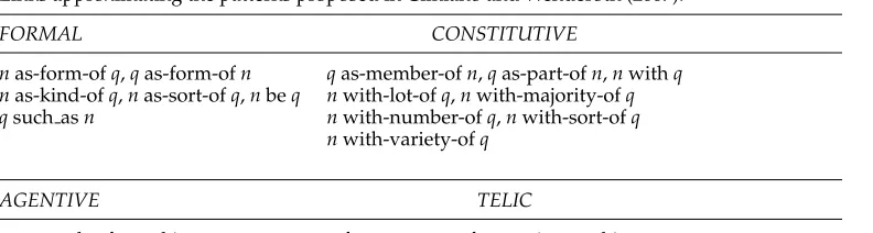
attribute noun: one of 127 nouns extracted from WordNet and expressing attributes of concepts, such assize,color, orheight. This pattern connects adjectives and nouns that occur in the templates(the) attribute noun of (a|the) NOUN is ADJ(Almuhareb and Poesio 2004) and(a|the) ADJ

attribute noun of NOUN(Veale and Hao 2008):the color of strawberries is red→ red,color+j+ns, strawberry;the autumnal color of the forest→ autumnal,

color+j+n-the, forest;

as adj as: this pattern links an adjective and a noun that match the templateas ADJ as (a|the) NOUN(Veale and Hao 2008):as sharp as a knife→ sharp,

as adj as+j+n-a, knife;

such as: links two nouns occurring in the templatesNOUN such as NOUNand such NOUN as NOUN(Hearst 1992, 1998):animals such as cats→

The scoring function σ is the same as that in DepDM, and the number of non-zero tuples is about 355M, including direct and inverse links. LexDM is a 30,693× 3,352,148×30,693 tensor with density 0.00001%.

TypeDM.This model is based on the idea, motivated and tested by Baroni et al. (2010)— but see also Davidov and Rappoport (2008a, 2008b) for a related method—that what matters is not so much the frequency of a link, but the variety of surface forms that express it. For example, if we just look at frequency of co-occurrence (or strength of association), the triplefat, of−1, land(a figurative expression) is much more common than the semantically more informative fat, of−1, animal. However, if we count the different surface realizations of the former pattern in our corpus, we find that there are only three of them (the fat of the land,the fat of the ADJ land, andthe ADJ fat of the land), whereasfat, of−1, animalhas nine distinct realizations (a fat of the animal,the fat of the animal,fats of animal,fats of the animal,fats of the animals,ADJ fats of the animal, andthe fats of the animal). TypeDM formalizes this intuition by adopting as links the patterns inside the LexDM links, while the suffixes of these patterns are used to count their number of distinct surface realizations. We call the model TypeDM because it counts typesof realizations, not tokens. For instance, the two LexDM linksof−1+n-a+n-theandof−1 +ns-j+n-theare counted as two occurrences of the same TypeDM linkof−1, corresponding to the pattern in the two original links.

The scoring function σ computes LMI not on the raw word–link–word co-occurrence counts, but on the number of distinct suffix types displayed by a link when it co-occurs with the relevant words. For instance, a TypeDM link derived from a LexDM pattern that occurs with nine different suffix types in the corpus is assigned a frequency of 9 for the purpose of the computation of LMI. The distinct TypeDM links are 25,336. The number of non-zero tuples in the TypeDM tensor is about 130M, including direct and inverse links. TypeDM is a 30, 693×25, 336×30, 693 tensor with density 0.0005%.

To sum up, the three DM instance models herein differ in the degree of lexicali-zation of the link set, and/or in the scoring function. LexDM is a heavily lexicalized model, contrasting with DepDM, which has a minimum degree of lexicalization, and consequently the smallest set of links. TypeDM represents a sort of middle level both for the kind and the number of links. These consist of syntactic and lexicalized patterns, as in LexDM. The lexical information encoded in the LexDM suffixes, however, is not used to generate different links, but to implement a different counting scheme as part of a different scoring function.

A weighted tuple structure (equivalently: a labeled DM tensor) is intended as a long-term semantic resource that can be used in different projects for different tasks, analogously to traditional hand-coded resources such as WordNet. Coherent with this approach, we make our best DM model (TypeDM) publicly available from http://clic.cimec.unitn.it/dm. The site also contains a set of Perl scripts that per-form the basic operations on the tensor and its derived vectors we are about to describe.

5.2 Semantic Vector Manipulation

geometric framework we adopt, and suffice to face all the tasks we will deal with (the decomposition techniques explored in Section 6.5 are briefly introduced there).

Vector length and normalization.The length of a vectorvwith dimensionsv1,v2,. . .,vnis:

||v||=i

=n

i=1v

2 i

A vector is normalized to have length 1by dividing each dimension by the original vector length.

Cosine.We measure the similarity of two vectorsxandyby the cosine of the angle they form:

cos(x,y)=

i=n i=1xiyi ||x||||y||

The cosine ranges from±1for vectors pointing in the same direction to 0 for orthogonal vectors. Other similarity measures, such as Lin’s measure (Lin 1998b), work better than the cosine in some tasks (Curran and Moens 2002; Pad ´o and Lapata 2007). However, the cosine is the most natural similarity measure in the geometric formalism we are adopting, and we stick to it as the default approach to measuring similarity.

Vector sum.Two or more vectors are summed in the obvious way, by adding their values on each dimension. We always normalize the vectors before summing. The resulting vector points in the same direction as the average of the summed normalized vectors. We refer to it as thecentroidof the vectors.

Projection onto a subspace.It is sometimes useful to measure length or compare vectors by taking only some of their dimensions into account. For example, one way to find nouns that are typical objects of the verbto singis to measure the length of nouns in aW1×LW2

subspace in which only dimensions such asobj, singhave non-0 values. We project a vector onto a subspace of this kind through multiplication of the vector by a square diagonal matrix with 1s in the diagonal cells corresponding to the dimensions we want to preserve and 0s elsewhere. A matrix of this sort performs an orthogonal projection of the vector it multiplies (Meyer 2000, chapter 5).

6. Semantic Experiments with the DM Spaces

The choice of the DM semantic space to tackle a particular task is essentially based on the “naturalness” with which the task can be modeled in that space. However, alternatives are conceivable, both with respect to space selection, and to the operations performed on the space. For instance, Turney (2008) models synonymy detection with a DSM that closely resembles our W₁W₂×L space, whereas we tackle this task under the more standardW₁×LW₂ view. It is an open question whether there are principled ways to select the optimal space configuration for a given semantic task. In this article, we limit ourselves to proving that each space derived through tensor matricization is semantically interesting in the sense that it provides the proper ground to address some semantic task.

Feature selection/reweighting and dimensionality reduction have been shown to improve DSM performance. For instance, the feature bootstrapping method proposed by Zhitomirsky-Geffet and Dagan (2009) boosts the precision of a DSM in lexical en-tailment recognition. Even if these methods can be applied to DM as well, we did not use them in our experiments. The results presented subsequently should be regarded as a “baseline” performance that could be enhanced in future work by exploring various task-specific parameters (we will come back in the conclusion to the role of parameter tuning in DM). This is consistent with our current aim of focusing on the generality and adaptivity of DM, rather than on task-specific optimization. As a first, important step in this latter direction, however, we conclude the empirical evaluation in Section 6.5 by replicating one experiment using tensor-decomposition-based smoothing, a form of optimization that can only be performed within the tensor-based approach to DSMs.

In order to maximize coverage of the experimental test sets, they are pre-processed with a mixture of manual and heuristic procedures to assign a POS to the words they contain, lemmatize, convert some multiword forms to single words, and turn some ad-verbs into adjectives (our models do not contain multiwords or adad-verbs). Nevertheless, some words (or word pairs) are unrecoverable, and in such cases we make a random guess (in cases where we do not have full coverage of a data set, the reported results are averages across repeated experiments, to account for the variability in random guesses). In many of the experiments herein, DM is not only compared to the results avail-able in the literature, but also to our implementation of state-of-the-art DSMs. These alternative models have been trained on the same corpus (with the same linguistic pre-processing) used to build the DM tuple tensors. This way, we aim at achieving a fairer comparison with alternative approaches in distributional semantics, abstracting away from the effects induced by differences in the training data.

Most experiments report global (micro-averaged) test set accuracy (alone, or com-bined with other measures) to assess the performance of the algorithms. The number of correctly classified items among all test elements can be seen as a binomially distributed random variable, and we follow the ACL Wiki state-of-the-art site7 in reporting also Clopper–Pearson binomial 95% confidence intervals around the accuracies (binomial intervals and other statistical quantities were computed using the R package;8where no further references are given, we used the standard R functions for the relevant analysis). The binomial confidence intervals give a sense of the spread of plausible population values around the test-set-based point estimates of accuracy. Where appropriate and interesting, we compare the accuracy of two specific models statistically with an exact Fisher test on the contingency table of correct and wrong responses given by the two

models. This approach to significance testing is problematic in many respects, the most important being that we ignore dependencies in correct and wrong counts due to the fact that the algorithms are evaluated on the same test set (Dietterich 1998). More appropriate tests, however, would require access to the fully itemized results from the compared algorithms, whereas in most cases we only know the point estimate reported in the earlier literature. For similar reasons, we do not make significance claims regard-ing other performance measures, such as macro-averaged F. Other forms of statistical analysis of the results are introduced herein when they are used; they are mostly limited to the models for which we have full access to the results. Note that we are interested in whether DM performance is overall within state-of-the-art range, and not on making precise claims about the models it outperforms. In this respect, we think that our general results are clear even where they are not supported by statistical inference, or interpretation of the latter is problematic.

6.1 TheW1×LW2Space

The vectors of this space are labeled with wordsw1(rows of matrixAmode-1in Table 3),

and their dimensions are labeled with binary tuples of typel,w2(columns of the same

matrix). The dimensions represent the attributes of words in terms of lexico-syntactic relations with lexical collocates, such assbj intr, read, or use, gun. Consistently, all the semantic tasks that we address with this space involve the measurement of the attributional similarity between words.

TheW₁×LW₂matrix is a structured semantic space similar to those used by Curran and Moens (2002), Grefenstette (1994), and Lin (1998a), among others. To test if the use of links detracts from performance on attributional similarity tasks, we trained on our concatenated corpus two alternative models—Win and DV—whose features only include lexical collocates of the target. Win is an unstructured DSM that does not rely on syntactic structure to select the collocates, but just on their linear proximity to the targets (Lund and Burgess 1996; Sch ¨utze 1997; Bullinaria and Levy 2007, and many others). Its matrix is based on co-occurrences of the same 30K words we used for the other models within a window of maximally five content words before or after the target. DV is an implementation of the Dependency Vectors approach of Pad ´o and Lapata (2007). It is a structured DSM, but dependency paths are used to pick collocates, without being part of the attributes. The DV model is obtained from the same co-occurrence data as DepDM (thus, relying on the dependency paths we picked, not the ones originally selected by Pad ´o and Lapata for their tests). Frequencies are summed across dependency path links for word–link–word triples with the same first and second words. Suppose that soldierandgunoccur in the tuplessoldier, have, gun(frequency 3) andsoldier, use, gun (frequency 37). In DepDM, this results in two features forsoldier:have, gunanduse, gun. In DV, we would derive a singlegunfeature with frequency 40. As for the DM models, the Win and DV counts are converted to LMI weights, and negative LMI values are raised to 0. Win is a 30,693×30,693 matrix with about 110 million non-zero entries (density: 11.5%). DV is a 30,693×30,693 matrix with about 38 million non-zero values (density: 4%).

in the W1×LW2 space between the nouns in each pair correlate with the ratings. The

results (expressed in terms of percentage correlations) are presented in Table 4, which also reports state-of-the-art performance levels of corpus-based systems from the litera-ture (the correlation of all systems with the ratings is very significantly above chance, according to a two-tailed t-test for Pearson correlation coefficients;df =63, p<0.0001 for all systems).

One of the DM models, namely TypeDM, does very well on this task, outperformed only by DoubleCheck, an unstructured system that relies on Web queries (and thus on a much larger corpus) and for which we report the best result across parameter settings. We also report the best results from a range of experiments with different models and parameter settings from Herda ˇgdelen, Erk, and Baroni (2009) (whose corpus is about half the size of ours) and Pad ´o and Lapata (2007) (who use a much smaller corpus). For the latter, we also report the best result they obtain when using cosine as the similarity measure (cosDV-07). Overall, the TypeDM result is in line with the state of the art, given the size of the input corpus, and the fact that we did not perform any tuning. Following Pad ´o, Pad ´o, and Erk (2007) we used the approximate test proposed by Raghunathan (2003) to compare the correlations with the human ratings of sets of models (this is only possible for the models we developed, as the test requires computation of correlation co-efficients across models). The test suggests that the difference in correlation with human ratings between TypeDM and our second best model, Win, is significant (Q=4.55,df =

0.23, p<0.01). On the other hand, there is no significant difference across Win, DepDM, DV and LexDM (Q=1.02,df =1.80, p=0.55).

6.1.2 Synonym Detection.The previous experiment assessed how the models can simu-late quantitative similarity ratings. The classic TOEFL synonym detection task focuses on the high end of the similarity scale, asking the models to make a discrete decision about which word is the synonym from a set of candidates. The data set, introduced to computational linguistics by Landauer and Dumais (1997), consists of 80 multiple-choice questions, each made of a target word (a noun, verb, adjective, or adverb) and four candidates. For example, given the targetlevied, the candidates areimposed,believed, requested, correlated, the first one being the correct choice. Our algorithms pick the candidate with the highest cosine to the target item as their guess of the right synonym. Table 5 reports results (percentage accuracies) on the TOEFL set for our models as well as the best model of Herda ˇgdelen and Baroni (2009) and the corpus-based models from the ACL Wiki TOEFL state-of-the-art table (we do not include those models from the Wiki that resort to other knowledge sources, such as WordNet or a thesaurus). The claims to follow about the relative performance of the models must be interpreted cautiously, in light of the spread of the confidence intervals: It suffices to note that,

Table 4

Percentage Pearson correlation with the Rubenstein and Goodenough (1965) similarity ratings.

model r model r model r

DoubleCheck1 85 Win 65 DV 57

TypeDM 82 DV-073 62 LexDM 53

SVD-092 80 DepDM 57 cosDV-073 47

Table 5

Percentage accuracy in TOEFL synonym detection with 95% binomial confidence intervals (CI).

model accuracy 95% CI model accuracy 95% CI

LSA-031 92.50 84.39–97.20 DepDM 75.0164.06–84.01

GLSA2 86.25 76.73–92.93 LexDM 74.37 63.39–83.49

PPMIC3 85.00 75.26–92.00 PMI-IR-018 73.75 62.72–82.96 CWO4 82.55 72.38–90.09 DV-079 73.00 62.72–82.96 PMI-IR-035 81.25 70.97–89.11 Win 69.37 58.07–79.20 BagPack6 80.00 69.56–88.11 Human10 64.50 53.01–74.88

DV 76.87 66.10–85.57 LSA-9710 64.38 52.90–74.80

TypeDM 76.87 66.10–85.57 Random 25.00 15.99–35.94 PairClass7 76.25 65.42–85.05

Model sources:1_{Rapp (2003);}2_{Matveeva et al. (2005);}3_{Bullinaria and Levy (2007);}4_Ruiz-Casado, Alfonseca, and Castells (2005);5Terra and Clarke (2003);6Herda ˇgdelen and Baroni (2009);7Turney (2008);8Turney (2001);9Pad ´o and Lapata (2007);10Landauer and Dumais (1997).

according to a Fisher test, the difference between the second-best model, GLSA, and the twelfth model, PMI-IR-01, is not significant at theα=.05 level (p=0.07). The difference between the bottom model, LSA-97, and random guessing is, on the other hand, highly significant (p< .00001).

The best DM model is again TypeDM, which also outperforms Turney’s unified PairClass approach (supervised, and relying on a much larger corpus), as well as his Web-statistics based PMI-IR-01model. TypeDM does better than the best Pad ´o and Lapata model (DV-07), and comparably to our DV implementation. Its accuracy is more than 10% higher than the average human test taker and the classic LSA model (LSA-97). Among the approaches that outperform TypeDM, BagPack is supervised, and CWO and PMI-IR-03 rely on much larger corpora. This leaves us with three unsupervised (and unstructured) models from the literature that outperform TypeDM while being trained on comparable or smaller corpora: LSA-03, GLSA, and PPMIC. In all three cases, the authors show that parameter tuning is beneficial in attaining the reported best performance. Further work should investigate how we could improve TypeDM by exploring various parameter settings (many of which do not require going back to the corpus: feature selection and reweighting, SVD, etc.).